HAL Id: inserm-00156907
https://www.hal.inserm.fr/inserm-00156907
Submitted on 25 Jun 2007HAL is a multi-disciplinary open access archive for the deposit and dissemination of sci-entific research documents, whether they are pub-lished or not. The documents may come from teaching and research institutions in France or
L’archive ouverte pluridisciplinaire HAL, est destinée au dépôt et à la diffusion de documents scientifiques de niveau recherche, publiés ou non, émanant des établissements d’enseignement et de recherche français ou étrangers, des laboratoires
Estimation of population pharmacokinetic parameters of
saquinavir in HIV patients with the MONOLIX
software.
Marc Lavielle, France Mentré
To cite this version:
Marc Lavielle, France Mentré. Estimation of population pharmacokinetic parameters of saquinavir in HIV patients with the MONOLIX software.. Journal of Pharmacokinetics and Pharmacodynamics, Springer Verlag, 2007, 34 (2), pp.229-49. �10.1007/s10928-006-9043-z�. �inserm-00156907�
Estimation of population pharmacokinetic parameters of
saquinavir in HIV patients with the MONOLIX software
Marc Lavielle1, France Mentré2,3
1
Department of Mathematics, University Paris 11 & University Paris 5, France, 2INSERM, U738, Paris, France
3University Paris 7, Dept of Epidemiology, Biostatistics and Clinical Research, Paris, France
Running title: Population pharmacokinetics of saquinavir with MONOLIX
Corresponding author: Marc Lavielle, Bât 425, Laboratoire de Mathématiques, Université Paris 11, 91400 Orsay France Tel: (33) 1 69 15 57 43 Fax : 33 1 69 15 72 34 E-mail: [email protected] Key-words:
EM algorithm, nonlinear mixed-effects models, stochastic approximation, importance sampling, model selection, pharmacokinetics, saquinavir.
HAL author manuscript inserm-00156907, version 1
HAL author manuscript
Abstract
In nonlinear mixed-effects models, estimation methods based on a linearization of the likelihood are widely used although they have several methodological drawbacks. Kuhn and Lavielle (2005) developed an estimation method which combines the SAEM (Stochastic Approximation EM) algorithm, with a MCMC (Markov Chain Monte Carlo) procedure for maximum likelihood estimation in nonlinear mixed-effects models without linearization. This method is implemented in the Matlab software MONOLIX which is available at http://www.math.u-psud.fr/~lavielle/monolix/logiciels. In this paper we apply MONOLIX to the analysis of the pharmacokinetics of saquinavir, a protease inhibitor, from concentrations measured after single dose administration in 100 HIV patients, some with advance disease. We also illustrate how to use MONOLIX to build the covariate model using the Bayesian Information Criterion. Saquinavir oral clearance (CL/F) was estimated to be 1.26 L/h and to increase with body mass index, the inter-patient variability for CL/F being 120%. Several methodological developments are ongoing to extend SAEM which is a very promising estimation method for population pharmacockinetic / pharmacodynamic analyses.
Introduction
Population pharmacokinetics (PK) and pharmacodynamics are increasingly performed in drug development and for therapeutic drug monitoring. They are based on nonlinear mixed-effects models (NLMEM) and the most popular software in that area is NONMEM which was developed by Lewis Sheiner and Stuart Beal (1). In these mixed-effects models, the problem is that the individual random mixed-effects are not observed and should be treated as missing data. The usual statistical approach is to integrate them out of the joint distribution of the response and the random effects in order to allow maximum likelihood estimation. However, for models that are nonlinear with respect to the parameters, this integral does not in general have a closed form expression and the first ideas was to used first-order approximations. The First-Order (FO) method was developed in NONMEM in 1977 (2). The first order conditional estimation method (FOCE) was arguably the most significant parametric method to emerge after. Davidian and Giltinan (3) explained in detail the technical differences between the various FOCE approaches as well as their implementation in various software applications and more recent complex approximations. These methods based on an approximated model are not true maximum likelihood estimation methods, so that all the nice statistical properties of maximum likelihood estimators are not true although they are applied in practice, e.g. standard errors derived from the Fisher information matrix, confidence intervals based on normality of the estimators, likelihood ratio test for nested models and Akaike criterion for model comparisons. Also, inconsistency of the FOCE estimators was demonstrated when the number of subjects increases with a fixed number of observations per subject (4, 5), although it was shown that it was not that bad when the residual error variance is "small" compare to the inter-individual variability (6).
The EM algorithm was first proposed and developed for problems with missing data. These are two-step algorithms: the E-step for conditional expectation of the needed statistics for the complete data likelihood given the observed data, and the M-step for maximum likelihood of the complete data (7). They were applied to linear mixed-effects models considering the random effects as the missing data (8). However, again because of the nonlinear structural model, there was no clear extension of the EM algorithm to NLMEM except with approximation during the E-step (9).
The Bayesian approach fro NLMEM was the first to use computer intensive procedures based on Markov Chain Monte Carlo (MCMC) techniques in order to propose a solution without approximation. As new and much more rapid software and statistical developments became available, interest grew.
In the maximum likelihood framework, Wei and Tanner (10), Walker (11) and Wu (12, 13) propose a Monte Carlo EM (MCEM) where the intractable E-step of EM is approximated with an empirical average based on simulated data. Unfortunately, MCEM is very time-consuming in computation since it requires a huge amount of simulated data. Alternatively, Delyon et al. (14) introduced a stochastic approximation version of EM (SAEM), which is more efficient in terms of computation. The stochastic approximation method achieves an approximation to the E-step by computing a weighted average of the approximation in the current iteration and the ones from all the previous iterations. Delyon et al. (14) show that this method converges to the maximum likelihood estimate under very general conditions.
Kuhn and Lavielle (15) develop for NLMEM an algorithm which combined the SAEM (stochastic approximation version of EM) algorithm (14), with a Markov Chain Monte Carlo procedure. They showed the good statistical convergence properties of
Fisher information matrix. Then, the inverse of this estimated Fisher information matrix provides an estimate of the variance of the maximum likelihood estimator.
Model selection using AIC and/or BIC and hypothesis testing using the log-likelihood ratio test (LRT) require the computation of the log-likelihood of the observations under the various models tested. The likelihood however is particularly complex and has no close form for nonlinear models. It is accurately estimated by Monte-Carlo approaches, using an importance sampling method to reduce the variance of the estimation.
Lavielle developed in 2005 the software MONOLIX which implements this algorithm for maximum likelihood estimation in NLMEM without linearization. This Matlab software is available at http://www.math.u-psud.fr/~lavielle/monolix/logiciels. The objective of this software is to perform: 1) parameter estimation by computing the maximum likelihood estimator of the parameters without any approximation of the model (linearization, quadrature approximation...) and standard errors for the maximum likelihood estimator; 2) model selection by comparing several models using some information criteria (AIC, BIC), or testing hypotheses using the Likelihood Ratio Test, or testing parameters using the Wald Test; 3) goodness of fit plots; 4) data simulation. Because of the absence of linearization in the estimation method, the results are true maximum likelihood estimates for which all the statistical properties applied.
Saquinavir (SQV) is a protease inhibitor used in treatment of HIV patients. As for all protease inhibitors, there is a large PK inter-patient variability. To study more specifically the sources of the large inter-patient PK variability, a specific mono-centric trial was performed in patients which received a single dose of saquinavir (16). In order to get large variability of the covariates in the studied sample, patients from three different groups were included (see Methods).
The objectives of the present study were to apply and illustrate MONOLIX on a real data set, to estimate the population pharmacokinetic parameter of saquinavir in HIV patients in a global population analysis and to test the effects of several covariates on saquinavir pharmacokinetics. These data have been previously analyzed with a population approach using P-Pharm (9) but with a separate analysis in each group of patients, the relationship with covariates being in a second step performed on the Empirical Bayes estimates (EBE) of the individual parameters. The same statistical model was used with MONOLIX but a preliminary analysis of the data with another software is of course not necessary.
The aim of this paper is not to compare MONOLIX and the SAEM algorithm with other existing estimation methods but to show with a real and rather difficult PK example that maximum likelihood estimation and model selection is possible with this algorithm. Indeed, comparison of estimation methods should be done mainly on simulated data where the true answer is known. A blind simulation study comparing several software on simulated PK or PD data has been performed by Girard and Mentré and presented in 2005 (17); this study showed the very good estimation results of SAEM.
Methods
Data
Concentration data were obtained after single administration of 600 mg of SQV-HCV alone after a breakfast including 200 ml of grapefruit juice to enhance SQV absorption, in 100 HIV patients who never received protease inhibitor before (16). Each patient had three samples collected in 3 periods: 0 to 1.5 h, 2 to 4 h, and 5 to 12
( ; ) ( ; )
ij ij i ij i ij
y f x g x
radioimmunoassay. The trial design and evaluation biological measurement are more detailed in (16). Three groups of patient were enrolled in this prospective trial: i) asymptomatic patients, ii) AIDS symptomatic subjects without diarrhea, iii) AIDS symptomatic subjects with diarrhea, but we did not take into account this group effect here. Indeed, we focused our study to the estimation of the parameters and the selection of the covariate model.
Eleven covariates were recorded: gender, age, Body Mass Index (BMI), creatinine clearance (CLCR) estimated from serum creatinine using the Cokcroft and Gault formula, diarrhea (yes/no), mean weight of stools per 24 h, plasma albumine, xylose, lactulose/mannitol ratio (L/M), alkaline phosphate level (APL) and CD4 count. Xylose and L/M were obtained as described in (16) to evaluate intestinal absorption and permeability, respectively.
Statistical Modelling
The nonlinear mixed effects model was defined as
ϕ
ϕ ε
= + 2~
(0,
)
ijN
ε
;σ
iA
i iwhere f is the parametric function of the structural model, g is the parametric function for the error model, yij is the jth observation in the ith subject, φI is the p-dimensional
vector of model parameters for the ith subject, xij are the design variables for the jth
observation in the ith subject, εij is the residual error for the jth observation, in the ith
subject and σ2 is the variance of the residual unidentified variability. In most cases g=f, i.e. a proportional error model, or g=1, i.e. an additive error model.
The random effect and covariate model was defined as
(
)
φ
=
μ η
+
, . .~ 0, i i i dNη
Ω , i=1, …, N,i
A
where is the covariate (or design) matrix for the ith subject and assumed to be known,
μ
is a d-vector of fixed population parameters,η
i is a p-vector of random effects, Ω is the pxp variance-covariance matrix of the random effect parameters. Theunknown set of parameters of the model is
θ
=(
μ
, ,Ωσ
2)
which is of size P.As in [16], a one compartment model with first order absorption after a time-lag was used to model saquinavir pharmacokinetics:
(
)
( , ; ,
,
,
)
exp
(
)
exp
(
)
f D t V Cl ka Tlag
t
Tlag
ka t
Tlag
V
ka
Cl
V
+ +D ka
×
⎡
Cl
⎤
=
⎢
⎜
⎛
−
−
⎟
⎞
−
−
−
⎥
×
−
⎣
⎝
⎠
⎦
max(0, )
a
+=
a
(
i≤N,1≤ ≤j ni)
where D = 600 mg is the dose and t the time, and where . The design variables are xij = (Di , tij ) (cf remarques ci dessus).Because lognormally distributed
random effects for each PK parameter (V/F, CL/F, ka and Tlag) was assumed, the vector of Gaussian individual parameters φi was composed of the logarithm of V/F, CL/F, ka and Tlag. Two models for the variance of the residual error were tested (g=1 and g=f).
SAEM algorithm
We are in a classical framework of incomplete data: the observed data isy= yij,1≤ , whereas the random effects,
φ
=
(
φ
i,1
≤ ≤
i
N
)
, are the non observed data. Our purpose is to compute the maximum likelihood estimator of θ by maximizing the likelihood of the observationsl
(
y
,
θ
)
( )
.
In the case of a nonlinear function f, the E-step of the standard EM algorithm, that consists in computing
E log
(
(
,
( )k;
)
| ;
)
k
y
y
kQ
θ
=
p
φ θ
θ
, cannot be performed in aclosed-form. The SAEM (Stochastic Approximation version of EM algorithm), proposed
( )k
by Delyon et al. (14) consists in replacing the usual E-step of EM by a stochastic procedure (see Kuhn and Lavielle (15) and the user’s guide of MONOLIX for more details on SAEM). At iteration k, SAEM consists in three steps:
• Simulation-step: draw
φ
from the conditional distributionp(
. ;yθ
k−1)
.( )
• Stochastic approximation-step : update
Q
kθ
according to(
( )
( )
(
( ))
( )
)
1log
,
;
1 k k k k kQ
θ
=
Q
−θ
+
γ
p y
φ θ
−
Q
−θ
)
kwhere
(
γ
is a decreasing sequence of positive numbers.( )
max
k
Arg
θQ
k• Maximization-step : update
θ
k according toθ
=
θ
For NLMEM, the Simulation-step cannot be performed directly because
(
. ;
k 1)
p
y
θ
− cannot be found explicitly. To deal with this problem, Kuhn and Lavielle (15) propose to combine this algorithm with a MCMC (Markov chain Monte Carlo) procedure. The Hastings-Metropolis algorithm used in MONOLIX combines several proposal distributions: the marginal distributionsφ
i~
N A
(
iμ
k−1,
Ω
k−1)
. .
i i d and the
symmetric Gaussian distributions
(
( 1))
. .~ ,k
i i
i i dN
φ
φ
− Γ where Γ is a diagonal matrix suchthat the probability of acceptance is about 0.3.
It is recommended to set
γ
k=
1
for1
≤ ≤
k
K
and1
k
γ
=
k
−
K
fork
K
(thedefault value in MONOLIX is K=500). Indeed, the initial guess of
1
≥ +
θ
may be far from themaximum likelihood value we are looking for and the first K iterations with
γ
k=
1
allowthe method to converge quickly to a neighborhood of a maximum of the likelihood. Then, smaller step sizes ensure the almost sure convergence of the algorithm to this maximum. We combine this stochastic algorithm in MONOLIX with a Simulated
( ,1)k
Annealing procedure in order to avoid local maxima and converge to the global maximum likelihood estimator.
It is possible to slightly improve the results by running L Markov chains instead of only one (in MONOLIX, the default value is L=3). The Simulation-step then requires to draw L sequences
φ
, …, at iteration k and to combine stochastic approximation and Monte Carlo in the Stochastic approximation-step:( , )k L
φ
( )
( )
(
( , ))
( )
1 1 1log
,
k l;
k k k k lQ
Q
p y
Q
L
1
Lθ
γ
φ
θ
θ
− − =⎛
⎞
=
+
⎜
−
⎟
⎝
∑
⎠
θ
The complete log-likelihood can be written
(
)
( )
( )
( )
(
)
(
)
(
)
2
1
log , ; log 2 log log
2 2 2 1 1 tot tot N T ij n Np N n p y y f A A , 2 2 1 , log( ( ; )) ; 2 2 ( ; ) ij i i j ij i i i i i i i j ij i g x x g x
φ θ
π
φ
μ
−φ
μ
+ = − − Ω − − − −∑
− Ω − −∑
σ
φ
φ
σ
φ
= ⎛ ⎞ ⎜ ⎟ ⎜ ⎟ ⎝ ⎠∑
1 N tot i i n n = =∑
where is the total number of observations. If we consider a diagonal
covariance matrix Ω, , the Stochastic Approximation-step consists in updating the sufficient statistics of the complete model as follows:
(
( ))
, 1;
1, 2,...,
k is
i ki
N
γ φ
−−
−=
( ) ( ) 1 1 N T k k kc
=
c
−+
γ
⎛
⎜
φ φ
−
c
−⎞
⎟
⎝
∑
⎠
(
)
2 ( ) 1 1 ,;
k k k k ij ij i k i jr
=
r
−+
γ
⎜
⎛
⎣
⎡
y
−
f x
φ
⎦
⎤
−
r
−⎟
⎞
⎝
∑
⎠
, , 1 i k i k ks
=
s
+
1 k k k i i i=(
)
Here, si,k is a p-vector that approximates E
φ
i | ;yθ
k−1T i i i
E
⎜
∑
φ φ
⎟
(
)
2 1 ,;
| ;
ij ij i k i jE
⎛
⎜
⎡
⎣
y
−
f x
φ
⎤
⎦
y
θ
−⎞
⎟
⎝
∑
⎠
, ck is a p x p-matrix that approximates| ;
y
θ
k−1 and r⎛
⎞
⎝
⎠
,k is a scalar that approximates.
Then,
θ
k is obtained in the Maximization-step as follows: 1 N N T T , 1 1 k i i i i k i iA A
A s
μ
−⎛
⎞
=
∑
∑
= =⎜
⎟
⎝
⎠
,(
)
, ,(
)
(
)(
)
1 1 11
N N N T T T k k i k i k i k i k i k i k i i iDiag
c
A
s
s
A
A
A
N
=μ
=μ
=μ
μ
⎧
⎛
⎞
⎫
Ω =
⎨
⎜
−
−
+
⎟
⎬
⎝
⎠
⎩
∑
∑
∑
⎭
, 2 k k tot r nσ
= ,where Diag(A) is the diagonal matrix formed with the diagonal elements of A.
It is also possible to obtain an estimation of the Fisher information matrix using the Louis’ missing information principle (18, 15). This estimated Fisher information matrix converges to the true unknown observed Fisher information matrix when the number of iterations increases (see (15) for more details).The inverse of this information matrix provides an estimate of the variance of the maximum likelihood estimator and the standard errors are obtained without any approximation of the model. These standard errors can be used to perform directly a Wald test, for instance for the fixed-effects of covariates (19).
The likelihood is estimated by Importance Sampling also without any approximation of the model (15). Then, the likelihood ratio test can be used for testing the significance of a covariate in the model. For the test of a variance component to 0,
the asymptotic distribution of the likelihood ratio test under the null hypothesis is an even mixture of two chi-square distributions with 0 and 1 degree of freedom (20).
Individual estimates of the parameters are provided by MONOLIX as the mean of their posterior distribution. The standard deviations of this posterior distribution, i.e. the standard errors of these individual estimates are also provided.
Model Building
There is no real consensus on the way to do model building in population pharmacokinetics (21). We used an approach based on a full population analysis.
First an univariate analysis was performed using SAEM with the test of each covariate on each individual parameter using both a Wald test and a LRT test. Second, all population models with all combinations of covariates found significant in the univariate analysis were fitted and the best ones were chosen according to the Bayesian Information Criteria. This model selection procedure is decomposed in two stages: i) for a given dimension of the model, that is for a given number of covariates, select the model with the greatest likelihood (or several models if their likelihoods are very close), ii) compare these best models using an information criteria (we used BIC) for selecting the dimension of the final model.
Third we tested using both a Wald test and a LRT whether each covariate that remained in the final model was significant and we looked at the change in interpatient and residual variability when this covariate was included or not.
Results
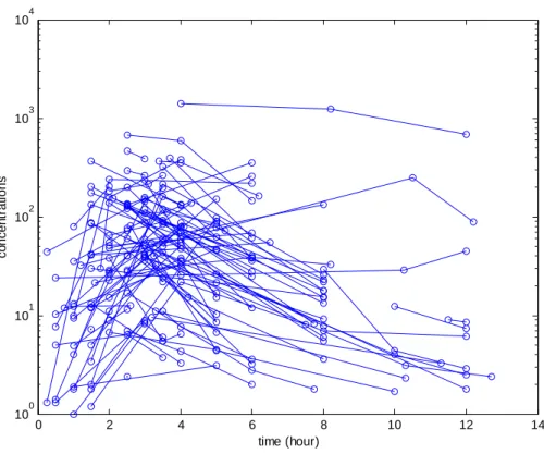
Observed concentrations of saquinavir are displayed Figure 1. Without any
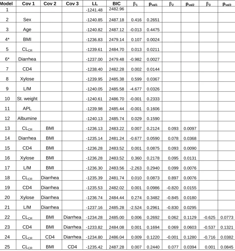
model as in Trout et al. (16). The Wald test and the LRT test also led us to keep random effects on all the parameters. SAEM as implemented in MONOLIX was able to estimate the four fixed effects and the variance of the four random effects with good precision. As in Trout et al. (16), the inter-patient variability was found to be very large especially for CL/F and V/F with coefficient of variations (CV), approximated as the standard deviation of η, of 127% and 176%, respectively. We then fit the eleven models with only one covariate in the model: in the univariate analysis, the Wald test and the LRT always agreed and six covariates were found to be significantly associated with CL/F (Table 1): BMI (p=0.0024), diarrhea (p=0.0027), CD4 count (p=0.014), creatinine clearance (p=0.021), lactose/mannitol ratio (p=0.033) and xylose (p=0.037). All these covariates are highly correlated and in Trout et al. (16), in the analysis of log(AUC), only BMI and log(xylose) were found to remain significant.
We then estimated with SAEM all the models with several of these six covariates (Table I). The lowest BIC was found for model 4 with only the covariate BMI which was positively associated with CL/F and with a change in BIC compared to the basic model with no covariate of 3.82 which can be considered as an important improvement (22). The second best model, model 6, had the effect of diarrhea decreasing CL/F and had a slightly higher BIC (change of 3.47). All models with two or more covariates had higher BIC and some of these models with BMI and/or diarrhea as a covariate are displayed in Table I. The best model with two covariates was with both BMI and diarrhea (model 14) but with a change of BIC from the basic model of only 1.1 and the Wald test for diarrhea was no longer significant. When BMI (diarrhea respectively) was incorporated in the model the inter-patient variability on CL/F dropped only to 119% (118% respectively) and inter-patient variability on V/F dropped to 156% (157% respectively). Because the model with BMI and the model with diarrhea
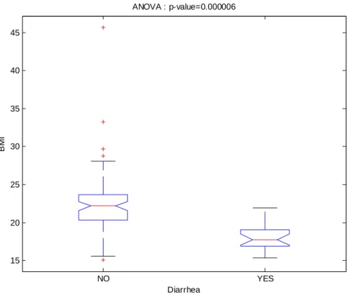
had very closed BIC we chose that to present the results of those two models. The choice of a final model between model 4 and model 6 depends on the purpose of the model building. The distribution of BMI conditionally to diarrhea is displayed Figure 2. We see that these two covariates are strongly negatively correlated: the BMI mean (SD) is 22.47 (0.42) in the group without diarrhea and 18.16 (0.80) in the group with diarrhea (p-value = 6 10-6).
The estimated parameters of these two models are given in Table II, and the standard errors of estimation were good even for all the inter-patient variances. The standard deviations of the residual error were 9.24 ng/ml (model 4) and 9.26 ng/ml (model 6) which is rather small compared to the range of observed concentrations.
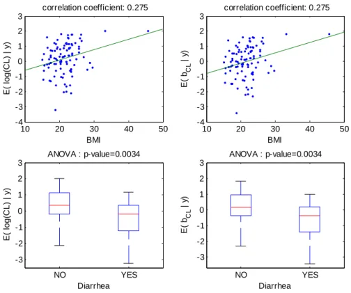
The increase (respectively decrease) of individual estimated values of log(CL/F) and of the corresponding random effect with BMI (respectively diarrhea) in the fitted model without covariate is displayed Figure 3. The model for CL/F without covariate is log(CL/F)=
μ
CL/F+bCL/F withμ
CL/F=0.23, then the left-hand and right-hand sides of this figure are identical, up to a shift on the y-axis ofμ
CL/F=0.23. These relationships obtained with model 4 (BMI as a single covariate) are displayed Figure 4. The relationship between log(CL/F) and BMI is well described with the linear model as no relationship remained between the individual random effects and BMI. Also, the means of log(CL/F) in the groups with and without diarrhea are significantly different but not the means of the individual random effects, which show that the model with BMI captures the diarrhea effect. Similar results obtained with model 6 (diarrhea as a single covariate) are displayed Figure 5, but it can be seen that with this model the BMI effect is not totally explained by diarrhea as some relationship between individual random effects and BMI remained.Several goodness of fit plots are displayed in Figure 6 and illustrate the quality of model 4 with BMI. Very similar goodness of fit plots are obtained with diarrhea instead of BMI.
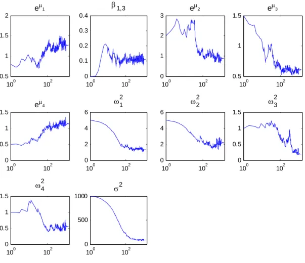
An example of the convergence of the SAEM algorithm for model 4 with BMI from rather poor estimate is displayed on Figure 7. In this example, the total number of iterations is 2000 decomposed into K=1000 iterations with γk = 1 and 1000 iterations with γk = 1/(k-1000). We used L = 5 independent Markov chains. Using these parameters, the computing time of the SAEM algorithm is about 1 minute on a labtop with a 1.6 GHz processor. A logarithmic scale is used for the x-axis to show that SAEM converges in very few iterations to a neighborhood of the maximum likelihood estimate when the stepsize γk = 1. The default values proposed in Monolix (L=3, K=300) are convenient for estimating roughly the parameters of the model, but not large enough in this example to compute accurate estimations of the standard errors and of the likelihood of the model.
Discussion
The results found on the population PK of saquinavir in this sample of patients are in accordance to those of the previous analysis (16), although we used here a different approach. Indeed we analyzed all the patients together and covariate model building was not based on individual estimates but on full population models at each step. We found that CL/F increased with BMI, or decreased with the presence of diarrhea which can be explained by a higher bioavailability of saquinavir in patients with severe body loss or diarrhea, although no effect was found of V/F. The physiological reasons have been discussed deeply by Trout et al. (16). The enhancement in
g( )
L
P
log(
n
tot)
saquinavir bioavailability could be due to the destruction of the transporters in enterocytes and/or to the enlargement of their tight junctions, allowing a paracellular crossing of saquinavir as the illness spreads. It should be noted that in this analysis, by construction of the three groups of inclusion, a third of the patient had severe body loss and/or diarrhea. The inter-patient variability of saquinavir was very high for V/F and CL/F even in the final models with BMI and/or diarrhea taken into account.
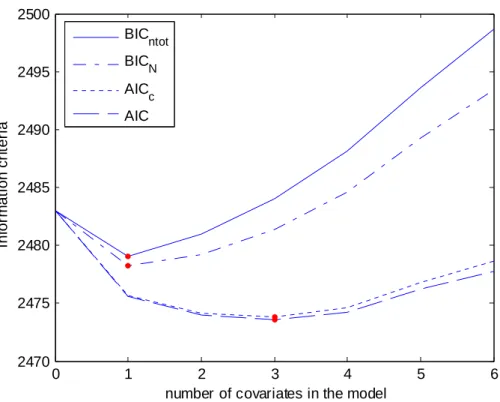
We defined the best error model based on the Bayesian Information Criteria which is usually defined in the literature (23) as
−
2 lo
+
2 log( ) 2
, where L is the likelihood, ntot the total number of observations and P the total number of parameters to
be estimated in the model. This choice is quite arbitrary and several other information criteria could be used. First, there is a discussion of which size should enter in the penalty function since BIC is a consistent criteria when the number of patients N increases. Thus, for testing the inclusion of covariates, the total number of patients N might be more appropriate than the total number of observations ntot in the penalization
term of BIC. The Akaike Information Criteria (AIC) defined as − L + Pis also very popular, but it is not consistent and usually overfits the model. AICc is a second order bias correction version of AIC defined as AICc = AIC + 2P(P+1)/(N-P+1) and that should be used instead of AIC when N is small (see 24 for more details). In AICc we use N for the correction but, as for BIC, it is not clear whether N or ntot should be chose.
These four different information criteria are displayed Figure 8 as a function of the number of covariates in the model with, for each number of covariate, the best model. We see that the model with the lowest BIC was the same with the two penalties (ntot or N) and includes only one covariate while the model with the lowest AIC and the lowest
AICc includes three covariates (model 23). This model has an effect of CD4, BMI and diarrhea, but with the Wald test none of these three covariates are significant,
illustrating the overfit described for model bulding based on AIC. A more complete analysis of these criteria is beyond the scope of this paper.
There is no real consensus on the strategy to perform model building in population PK/PD analysis and the number of models to evaluate could be quite large. For instance here there are four PK parameters and eleven covariates that were tested. We did a first screening of the covariate using the Wald test which had here similar results as the LRT. Further developments on covariate model building in nonlinear mixed effects models should be done and of course model selection depends of the purpose of the model.
One main feature of the SAEM algorithm is that it does not need an approximation of the likelihood. It is a stochastic extension of the EM algorithm. MONOLIX, which implements SAEM also provide an estimation of the likelihood and of the Fisher information matrix without linearization of the model so that both LRT and Wald test are more reliable then with estimation methods based on approximation of the likelihood. Similarly, the full posterior distribution of the random effects is computed and the EBE are defined as the mean of this distribution. MONOLIX also provides standard error on the EBE. Automatic and optimal choice of the parameters of the SAEM algorithm (number of iterations, sequence γk, number of chains…) is a rather
difficult problem. The default values proposed in MONOLIX 1.1 (L = 3, K = 300) were convenient for estimating roughly the parameters of the model but were not large enough to compute accurate estimations of the standard errors and of the likelihood of the model. It should be noted that this analysis presents a challenging problem in term of estimation, because the number of observations per individual (at most three) is smaller than the number of parameters in the PK model (four) and there is also a very large inter-patient variability.
Several extension of MONOLIX are under developments. First for models defined as ordinary differential equation we proposed to use a numerical procedure based on local linearization (25) to speed up the algorithm compared to standard Runge-Kutta numerical approximation methods (26). We are working on a version of MONOLIX that could handle left-censored data, as for instance concentration below the limit of quantification. Indeed these data can be considered as missing data and SAEM can be extended using the fact that they are additional missing data to the random effects. We are also working on the incorporation of a third level of variability to model for instance variability between occasions.
We also proposed to use MONOLIX in population design evaluation, for estimation of the expected information matrix without linearization (27) as an extension of PFIM based on a first-order linearization (28). A very large data set under the proposed design is simulated and then fitted with SAEM. The estimated information matrix from that fit is close to the expected information matrix and can easily be scaled to the number of patients that was initially scheduled.
In conclusion, as results of population PK/PD analyses are increasingly used for designing new trials, for instance trough clinical trial simulation, new methods without approximation of the likelihood that provides more reliable estimates and standard errors are needed. In the maximum likelihood framework extension to the EM algorithms have been proposed to that end (29). MONOLIX implements SAEM in Matlab and is a free software available at http://www.math.u-psud.fr/~lavielle. It is based on a thorough statistical theory (14, 15) and several statistical developments are ongoing. MONOLIX is a fast and efficient algorithm as illustrated in this real example with a sparse design and large inter-patient variability.
Acknowledgments
We thank Dr H. Trout and Pr J.F. Bergmann, Lariboisière Hospital, Paris, for the access to the data of the PK trial on saquinavir. MONOLIX software is developed by Marc Lavielle based on joint theoretical and applied works with several members of the MONOLIX Group (www.math.u-psud.fr/~lavielle/monolix). MONOLIX group is animated by Marc Lavielle and France Mentré. MONOLIX software is free and is protected by the terms of the GNU General Public License.
References
(1) S. L. Beal, L. B. Sheiner. The NONMEM System. Amer Statist 1980; 34:118-119. (2) L. B. Sheiner, B. Rosenberg, V. V. Marathe. Estimation of population characteristics
of pharmacokinetic parameters from routine clinical data. J Pharmacokinet Biopharm 1977; 5:445-479.
(3) M. Davidian, D. M. Giltinan. Non linear models for repeated measurement data: an overview and update. J Agric Biol Environ Stat 2003; 8:387-419.
(4) R. Q. Ramos, S. G. Pantula. Estimation of nonlinear random coefficient models. Statist Probab Letter 1995; 24: 49-56.
(5) E. F. Vonesh. A note on the use of Laplace's approximation for nonlinear mixed-effects models Biometrika, 1996; 83:447-52.
(6) H. Ko, M. Davidian. Correcting for measurement error in individual-level covariates in nonlinear mixed effect models. Biometrics 2000; 56:368-75.
(7) A. P. Dempster, N. M. Laird, D. B. Rubin. Maximum likelihood from incomplete data via the EM algorithm. J R Stat Soc Ser B Stat Methodol 1977; 1:1-38.
(8) M. J. Lindstrom, D. M. Bates. Newton-Raphson and EM algorithms for linear mixed-effects models for repeated-measures data. J Am Stat Assoc 1988; 83:1014-1022.
(9) F. Mentré, R. Gomeni. A two-step algorithm for estimation on non-linear mixed-effects with an evaluation in population pharmacokinetics. J Biopharm Stat 1995; 5:141-158.
(10) G. C. Wei, M. Z. Tanner MA. Applications of multiple imputation to the analysis of censored regression data. Biometrics 1991; 47:1297-1309.
(11) G. Walker. An EM algorithm for non-linear random effects models. Biometrics 1996; 52:934-944..
(12) L. Wu. A joint model for nonlinear mixed-effects models with censoring and covariates measured with error, with application to AIDS studies. J Amer Statist Assoc 2002; 97: 955-964.
(13) L. Wu. Exact and approximate inferences for nonlinear mixed-effects models with missing covariates. J Amer Statist Assoc 2004; 99: 700-709.
(14) B. Delyon, M. Lavielle, E. Moulines. Convergence os a stochastic approximation version of the EM procedure. Ann Stat 1999; 27:94-128.
(15) E. Kuhn, M. Lavielle. Maximum likelihood estimation in nonlinear mixed effects models. Comput Statist Data Anal 2005; 49:1020-1038.
(16) H. Trout, F. Mentré, X. Panhard, A. Kodjo, L. Escaut, P. Pernet, J.G. Gobert, D. Vittecoq, A.L. Knellwolf, C. Caulin and J.F. Bergmann. Enhanced saquinavir exposure in HIV1-infected patients with diarrhea and/or wasting syndrome. Antimicrob Agents Chemother 2004; 48: 538-545.
(17) P. Girard, F. Mentré. A comparison of estimation methods in nonlinear mixed effects models using a blind analysis. PAGE 14 2005; Abstr 834 [www.page-meeting.org/?abstract=834].
(18) T. A. Louis. Finding the observed information matrix when using EM algorithm. J R Stat Soc B, 1982; 44:226-233.
(19) K. G. Kowalski, M. M. Hutmacher. Efficient screening of covariates in population models using Wald's approximation to the likelihood ratio test. J Pharmacokinet Pharmacodyn 2001; 28:253-275.
(20) D. O. Stram, J. W. Lee. Variance components testing in the longitudinal mixed effects model. Biometrics 1994 ; 50(4):1171-1177. Erratum in: Biometrics 1995; 51(3):1196.
(21) E. N. Jonsson, M. O. Karlsson. Automated covariate model building within NONMEM. Pharm Res 1998; 15:1463-1468.
(22) R.E. Kass, A.E. Raftery. Bayes factors. J Am Stat Assoc 1995; 90:773-795.
(23) G. Verbeke, G. Molenberghs. Linear mixed effect models for longitudinal data. New York: Springer, 2004.
(24) K. P. Burnham, D. R. Anderson. Multimodel Inference: Understanding AIC and BIC in model selection. Sociological Methods & Research 2004; 33: 261-304. (25) J. I. Ramos. Linearized methods for ordinary differential equations. Appl Math
Comput 1999; 104: 109-129.
(26) A. Samson, X. Panhard, M. Lavielle, F. Mentré. Generalisation of the SAEM algorithm to nonlinear mixed effects model defined by differential equations: application to HIV viral dynamic models. PAGE 14 2005; Abstr 716 [www.page meeting.org/?abstract=716]
(27) S. Retout, E. Comets, A. Samson, F. Mentré. Designs in nonlinear mixed effects models: application to HIV viral load decrease with evaluation, optimization and determination of the power of the test of a treatment effect. PAGE 14 2005; Abstr 775 [www.page-meeting.org/?abstract=775]
(28) S. Retout, F. Mentré. Optimization of individual and population designs using Splus. J Pharmacokinet Pharmacodyn 2003; 30:417-443.
(29) G. C. Pillai GC, F. Mentré F, J. L.Steimer. Non-linear mixed effects modeling - from methodology and software development to driving implementation in drug development science. J Pharmacokinet Pharmacodyn. 2005; 32:161-183.
Table I: For the basic model and several models with one, two or three covariates
on log(CL/F): Log-likelihood (LL), BIC and estimated fixed effects (β) of the
covariates with the corresponding p-value of the Wald test
Model Cov 1 Cov 2 Cov 3 LL BIC β1 pval1 β2 pval2 β3 pval3
1 -1241.48 2482.96 2 Sex -1240.85 2487.18 0.416 0.2651 3 Age -1240.82 2487.12 -0.013 0.4475 4* BMI -1236.83 2479.14 0.107 0.0024 5 CLCR -1239.61 2484.70 0.013 0.0211 6* Diarrhea -1237.00 2479.48 -0.982 0.0027 7 CD4 -1238.40 2482.28 0.002 0.0144 8 Xylose -1239.95 2485.38 0.599 0.0367 9 L/M -1240.05 2485.58 -4.677 0.0326 10 St. weight -1240.61 2486.70 -0.001 0.2333 11 APL -1239.98 2485.44 -0.001 0.1606 12 Albumine -1240.13 2485.74 0.029 0.1590 13 CLCR BMI -1236.13 2483.22 0.007 0.2124 0.093 0.0097 14 Diarrhea BMI -1235.14 2481.24 -0.677 0.0590 0.078 0.0368 15 CD4 BMI -1236.28 2483.52 0.001 0.0875 0.093 0.0090 16 Xylose BMI -1236.28 2483.52 0.360 0.2178 0.095 0.0131 17 L/M BMI -1236.30 2483.56 -2.263 0.2940 0.099 0.0076 18 CLCR Diarrhea -1235.39 2481.74 0.010 0.0873 0.897 0.0076 19 CD4 Diarrhea -1235.53 2482.02 0.001 0.0986 -0.820 0.0155 20 Xylose Diarrhea -1236.74 2484.44 0.274 0.3482 -0.845 0.0180 21 L/M Diarrhea -1237.16 2485.28 -2.524 0.2961 -0.830 0.0295 22 CLCR BMI Diarrhea -1234.28 2485.00 0.006 0.2692 0.062 0.1129 -0.625 0.0773 23 CD4 BMI Diarrhea -1233.82 2484.08 0.001 0.1694 0.069 0.0603 -0.537 0.1321 24 CLCR CD4 Diarrhea -1234.80 2486.04 0.009 0.1220 -0.001 0.1280 -0.716 0.0382 25 CLCR BMI CD4 -1235.42 2487.28 0.007 0.2440 0.077 0.0394 0.001 0.0845
* The two models with the smallest BIC
Table II: Estimated population pharmacokinetic parameters of saquinavir with the two final modelsModel 4 Model 6 Estimate SE (CV %) Estimate SE (CV %) exp(μCL/F) in L/h 1.26 0.19 (15%) 1.25 0.18 (15%) βBMI_CL/F* 0.11 0.04 (33%) (p-value = 0.0024) βDIARRHEA_CL/F* -0.98 0.33 (33%) (p-value = 0.0027) exp(μV/F) in L 0.86 0.22 (26%) 0,96 0.24 (25%) exp(μka) in h-1 0.58 0.05 (9%) 0.61 0,05 (8%) exp(μTlag) in h 1.13 0.12 (11%) 1.12 0.12 (12%) ωCL/F2 1.41 0.30 (22%) 1.38 0.29 (21%) ωV/F2 2.43 0.65 (27%) 2.45 0.60 (24%) ωka2 0.22 0.07 (29%) 0.17 0.05 (28%) ωTlag2 0.51 0.13 (25%) 0.53 0.12 (23%) σ2 in (ng/ml)2 85.3 12.5 (15%) 85.7 12.8 (15%) *Effect on log(CL/F)
104 0 2 4 6 8 10 12 14 100 101 102 103 time (hour) c o ncen tr at ion s
Figure 1: Observed individual concentrations (in ng/ml) of saquinavir
NO YES 15 20 25 30 35 40 45 BM I Diarrhea ANOVA : p-value=0.000006
Figure 2: Distribution of BMI conditionally to diarrhea
10 20 30 40 50 -4 -3 -2 -1 0 1 2 3 correlation coefficient: 0.275 BMI E( lo g (CL ) | y ) 3 10 20 30 40 50 -4 -3 -2 -1 0 1 2 correlation coefficient: 0.275 BMI E( bCL | y ) NO YES -3 -2 -1 0 1 2 3 E( lo g (C L ) | y ) Diarrhea ANOVA : p-value=0.0034 NO YES -3 -2 -1 0 1 2 3 Diarrhea ANOVA : p-value=0.0034 E( bCL | y )
Figure 3: For model 1 fitted without any covariate, relationships between individual log(CL/F) and BMI (top left), individual random effects for log(CL/F) and BMI (top right), individual log(CL/F) and diarrhea (bottom left), individual random effects for log(CL/F) and diarrhea (bottom right).
10 20 30 40 50 -4 -2 0 2 4 correlation coefficient: 0.443 BMI E( lo g (CL ) | y ) 4 10 20 30 40 50 -4 -2 0 2 correlation coefficient: -0.000 BMI E( b CL | y ) NO YES -3 -2 -1 0 1 2 3 E( lo g (C L ) | y ) Diarrhea ANOVA : p-value=0.0007 NO YES -3 -2 -1 0 1 2 3 Diarrhea ANOVA : p-value=0.1202 E( b CL | y )
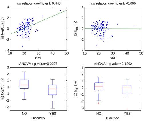
Figure 4: For model 4 fitted with the covariate BMI on log(CL/F), relationships between individual log(CL/F) and BMI (top left), individual random effects for log(CL/F) and BMI (top right), individual log(CL/F) and diarrhea (bottom left), individual random effects for log(CL/F) and diarrhea (bottom right).
10 20 30 40 50 -4 -3 -2 -1 0 1 2 3 correlation coefficient: 0.314 BMI E( lo g (CL ) | y ) 10 20 30 40 50 -4 -3 -2 -1 0 1 2 3 correlation coefficient: 0.157 BMI E( bCL | y ) NO YES -3 -2 -1 0 1 2 3 E( lo g (C L ) | y ) Diarrhea ANOVA : p-value=0.0001 NO YES -2 -1 0 1 2 3 E( bCL | y ) Diarrhea ANOVA : p-value=0.9881
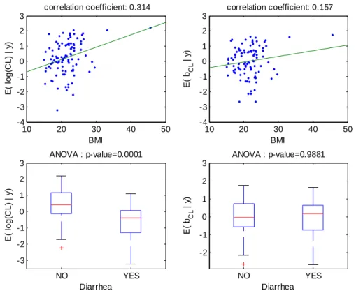
Figure 5: For model 6 fitted with the covariate diarrhea on log(CL/F), relationships between individual log(CL/F) and BMI (top left), individual random effects for log(CL/F) and BMI (top right), individual log(CL/F) and diarrhea (bottom left), individual random effects for log(CL/F) and diarrhea (bottom right).
0 500 1000 0 500 1000 ob s e rv ed c onc en tr a ti on s predicted concentrations Using the population parameters
0 500 1000 0 500 1000 ob s e rv ed c onc en tr a ti on s predicted concentrations Using the individual parameters
0 5 10 15 -500 0 500 1000 1500 time (hour) re si d u a ls 0 5 10 15 -100 -50 0 50 100 re si d u a ls time (hour)
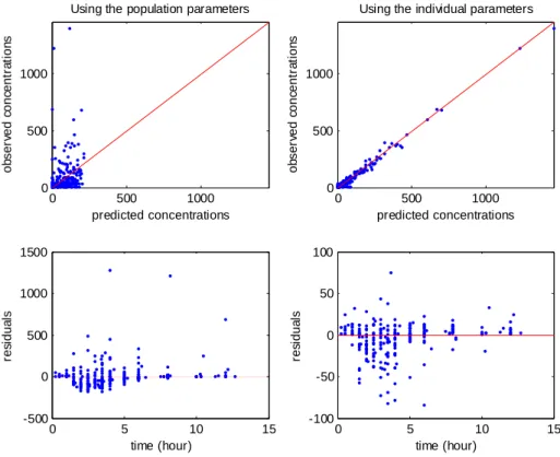
Figure 6: Goodness of fit plots for model 4 (BMI on CL/F). Top: observations versus predictions (in ng/ml), with on left population prediction and on right individual predictions; bottom: residuals versus time, with on left population residuals and on right individual residuals
100 102 0.5 1 1.5 2 eμ1 100 102 0 0.1 0.2 0.3 0.4 β1,3 100 102 0 1 2 3 eμ2 100 102 0.5 1 1.5 eμ3 100 102 0 0.5 1 1.5 eμ4 100 102 0 2 4 6 ω2 1 100 102 0 2 4 6 ω2 2 100 102 0 0.5 1 1.5 ω2 3 100 102 0 0.5 1 1.5 ω24 100 102 0 500 1000 σ2
Figure 7: Example of convergence of SAEM with model 4 from poor initial estimates
0 1 2 3 4 5 6 2470 2475 2480 2485 2490 2495 2500
number of covariates in the model
In fo rm at io n cr it er ia BICntot BICN AICc AIC
Figure 8: Four different Information criteria for selecting between 0 and 6 covariates: BIC using the total number of observations in the penalization term
(BICN), BIC using the number of individuals in the penalization term (BICntot), AIC
and corrected AIC (AICc).