Stochastic ordering based Markov process
aggregations : Application to tandem queues
Hind Castel
GET/INT/SAMOVAR INT
9,rue Charles Fourier 91011 Evry Cedex, France
Lynda Mokdad
Laboratoire Lamsade Universit´e de Paris Dauphine Place du Mar´echal de Lattre de Tassigny
75775 cedex 16, France [email protected]
Nihal Pekergin
Centre Marin Mersenne, Universit´e Paris 1, 90, Rue de Tolbiac, 75013 France PRISM, Universit´e Versailles-St Quentin
45, Av. des Etats Unis, 78038 France Email : [email protected]
Abstract— We present a general algorithm based on the sto-chastic ordering theory to provide a bounding aggregation for a given Markov process. Our main goal is to provide bounds on the performance measures of interest by considering the aggregated process without computing the exact values which are in general numerically difficult or intractable due to the well-known state space explosion. The stochastic comparison has been largely applied in performance evaluation however the state space is generally assumed to be totally ordered which provides less accurate bounds for multidimensional Markov processes. The algorithm is proposed by assuming a preorder on the state space, and it is applied in this paper to an open tandem queues system, in order to compute loss probabilities bounds.
keywords : multi-dimensional Markov processes, stochastic comparisons, tandem queues, loss probabilities.
I. INTRODUCTION
Actually, the growing complexity of telecommunication sys-tems make their performance evaluation by classical methods as simulation or mathematical analysis very difficult. We need new powerful mathematical tools for the quantitative analysis of multidimensional processes. In this paper, we focus on systems represented by multidimensional Markov processes. If the system has no specific solution form, since the state space increases exponentially, it will be very difficult or impossible to compute numerically the performance measures. We propose to use a mathematical method based on the stochastic comparisons of Markov processes. The key idea of this method is that given a complex Markov process which cannot be solved, we propose to bound it by a new Markov process which is easier to solve. A stochastic ordering is defined as a relation order between random variables, or stochastic processes [11]. The well-known stochastic ordering is the strong stochastic ordering (¹st). The stochastic ordering
theory can be also defined between processes represented on different state spaces by mapping functions on a common state space [5]. The stochastic comparison is an interesting mathematical tool for the performance evaluation of large size Markov processes. We use this methodology in order to define bounding Markov processes on a smaller state space, in order to compute bounds on performance measures. The advantage of this method is that it can be applied for many kinds of networks. We have already obtained some interesting results for mobile networks, MPLS/IP network, and optical networks. In [2], [1], we apply this method on mobile networks in order to obtain dropping handover bounds. In [4], we use it to compute loss rates packets in an optical switch, and in [3] for the loss rates packets in an IP switch. [10] presents in details this method and apply it to evaluate loss rates cells in an ATM switch. In this paper, we present a general
algorithm which generates a bounding Markov process as the aggregation version of a given large state space Markov process. We apply this algorithm to the analysis of an open tandem queues in order to evaluate the loss probabilities. This model has been frequently used, for instance to represent manufacturing queueing systems, and also in ATM networks to represent a virtual circuit. It is also used in IP networks as a model for a VPN [12]. We represent the tandem queue system by a Markov process which has not a closed-form solution. One way of analyzing such queueing is to solve numerically for the stationary probability vector of the Markov process. However memory complexity limits this approach to small queueing networks. Alternatively, when the number of queues in tandem increases, approximation algorithms can be used [9]. This paper is organized as follows. In the next section, we explain how to use the stochastic comparison for the state space reduction, and we give the main steps of the algorithm generating the aggregated Markov process, in section III we prove that this algorithm provides really an upper bound. In section IV, we apply the algorithm to the tandem queues in order to evaluate the loss probabilities. Analytical results presented in section V show that the methodology is really interesting. In section VI, we discuss the achieved results, and give comments about further research items. At the end, we present in the appendix some definitions and theorems about stochastic orderings.
II. STATE SPACE REDUCTION USING STOCHASTIC COMPARISON
The stochastic comparison is a mathematical tool which allows to compute bounds on transient distributions and the stationary distribution of a Markov process. In fact, if the un-derlying Markov process does not have a specific solution form like product-form, lumpability, matrix-geometric solutions, etc. the computation of transient and stationary probability distributions becomes difficult or intractable for large state spaces. By means of the stochastic comparison method, it is possible to overcome this problem by reducing the size of the state space of the underlying Markov process. We are interested in performance measures computed as an increasing reward function on the stationary distribution. In some cases (for example loss probabilities) this reward function depends only on few states :it equals 0 for a lot of states, and has a positive value for few states. So it is not necessary to represent all the states, and some of them can be put together (which are not used in the computation on the performance measure), in order to reduce the size of the state space. Let
on a partially ordered state space E, and R a performance measure computed on the stationary distribution Π of the process as follows :
R = X
x∈E
Π(x)f (x) (1)
where f is an increasing reward function according to the order defined on E. If there is no specific solution for Π, then it is very difficult or intractable to compute as the state space E is very large. So we reduce E by gathering some states thus by defining a many to one mapping Ag from E to S such that S ⊂
E. We build a new aggregated Markov process {Xb(t), t ≥
0} on S (with the stationary distribution Πb) defined as a
bounding Markov process, in order to compute :
Rb=X
x∈S
Πb(x)f (x) (2)
which is a lower or an upper bound for R. Aggregation is not performed on states x such that f (x) 6= 0, and f (x) has the same values in Rb than in R. Let us remark here that the aggregation is not applied to gather lumpable states to provide exact values but some state to provide bounding aggregation by means of the stochastic comparison. Xb(t) is defined on the state space S, with an infinitesimal generator matrix computed from the stochastic ordering theory [11],[5], [8], presented in the appendix. The definition of an aggre-gated bounding Markov process involves inequalities between stationary probability distributions Πb and Π. So we propose an attractive solution to the problem of computing R : we compute Rbon Πbwhich represents an upper or a lower value for R. Next, we present the algorithm which generates the aggregated bounding Markov process {Xb(t), t ≥ 0}. A. Definition of bounded Markov processes by aggregation
We have the following assumptions for the algorithm :
• {X(t), t ≥ 0} is a Markov process defined on a large state
space E, and Q is the infinitesimal generator matrix .
• {X(t), t ≥ 0} is irreducible, so the stationary distribution Π
exists, and R is the performance measure to compute as given in equation (1).
We have defined an algorithm which generates the aggre-gated Markov process {Xb(t), t ≥ 0} , with infinitesimal generator Qb on the state space S, providing an upper bound
Rb. This algorithm can be applied only if two conditions are
verified:
1- First, we need to define on the state space E a preorder
¹ compatible with R (R is written as an increasing reward
function f on Π according to ¹).
2-Secondly, {X(t), t ≥ 0} must be ¹st monotone (see
Definition 5 in the appendix ).
The main steps of the algorithm are the definition of the state space S of the aggregated Markov chain, and its infinitesimal generator Qb. It is defined by the following steps :
• First, we define the state space S of the aggregated Markov
process. We give the mapping function Ag ( E → S), as an increasing function. For xi∈ E, we have two cases :
1- One state xi of E is mapped into the same state xi of S.
So Ag(xi) = xi and xi is called a ”simple” state of S.
2- A set {x1, . . . , xn} of E is mapped into the state xn of S
(xn is the ”upper” state, which means that x1 ¹ x2. . . ¹ xn
). So Ag(x1) = . . . = Ag(xi) = . . . = Ag(xn) = xn, and xn
is called a ”macro” state of S. The choice of states in E which are made together is not simple. It is performed according to the performance measure R (states where f is not null are
not aggregated), and the quality of the bound (as we will see after). According to steps (1) and (2), we have defined the mapping Ag, and so the set S is such that S = Ag(E).
• Secondly, we define the infinitesimal generator Qb from Q
as follows : for a state x ∈ S we have that : Qb(x, ∗) =
Q(x, ∗)MAg, where MAg is defined as in the Theorem 1 of
the appendix.
Note that the aggregation is defined so as we obtain an irreducible Markov process {Xb(t), t ≥ 0}. Next, we prove that {Xb(t), t ≥ 0} is really an upper bound for {X(t), t ≥ 0}.
III. STOCHASTIC COMPARISONS PROOFS
Using the stochastic ordering theory presented in the ap-pendix, we prove now that by following this algorithm, we have that : {Ag(X(t)), t ≥ 0} ¹st{Xb(t), t ≥ 0}. Following
Theorem 1 (where g represents Ag, h is the identity function, and F = S) , we must establish the monotonicity and the comparison results. Since X(t) is ¹st-monotone, and Ag is
an increasing function, then Ag(X(t)) is ¹st-monotone (see
Definition 6 in the appendix). For the comparison, we must prove that ∀x ∈ E, y ∈ S | Ag(x) = y, QMAg(x, ∗) ¹st
Qb(y, ∗). We have two cases for a state y ∈ S :
• if y is a simple state, then y is the mapping of only one state y of E such that y = Ag(y), and in this case, we have
accord-ing to the definition of Qb, that : Qb(y, ∗) = Q(y, ∗)MAg so
for a simple state y we have that : Q(y, ∗)MAg¹stQb(y, ∗).
• if y is a macro state, then ∃x1, . . . xn ∈ E such that
Ag(x1) = . . . = Ag(xn) = y. As y represents the upper
state, then if xn º . . . , º x1, we have that y = xn. In this
case, Qb is defined as : Qb(y, ∗) = Q(xn, ∗)MAg.
As QMAg is ¹st-monotone, then we have according to the
Theorem 3: Q(x1, ∗)MAg ¹st . . . ¹st Q(xn, ∗)MAg, and
as Q(xn, ∗)MAg = Qb(y, ∗), so we have : ∀1 ≤ i ≤
n, Q(xi, ∗)MAg¹stQb(y, ∗). Then, for a macro state y ∈ S,
we have : Q(x, ∗)MAg¹stQb(y, ∗), ∀x ∈ E | Ag(x) = y.
As the inequality is satisfied for all states y ∈ S, then from the Theorem 1, we deduce that {Ag(X(t)), t ≥ 0} ¹st
{Xb(t), t ≥ 0}. As the stochastic comparison of stochastic
processes generates the stochastic comparison of transient and stationary probability distributions, then we deduce that : ΠMAg ¹st Πb. For all performance measures written as
increasing reward functions f on the stationary distributions Π or Πb (if we suppose that the aggregation is done on states
x ∈ E such that f (x) = 0), then we have that : R ≤ Rb.
IV. STUDY OF TANDEM QUEUES SYSTEM
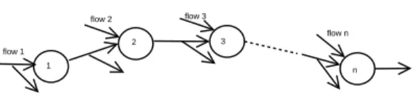
1 2 n 3 flow 1 flow 2 flow 3 flow n
Fig. 1. System understudy: a path in a network
The system understudy represents a path in a network defined as a series of network nodes (switches, routers) where transit different flows of packets. We suppose that the leftmost node has the index 1, and indexes increase in the path until node n. A flow of packets is defined by packets coming from the same source and going to the same final destination. All the flows have the same destination node (node n), if there is enough place in the nodes. For example, in Fig.1, we can see a flow coming from node 1, another from node 2,... etc we suppose that node n is the final destination of all the
flows if packets are not rejected in one of the nodes in the path. This system can be represented by n finite capacity queues in tandem. Queues are numbered from 1 to n starting from the leftmost queue. Each queue i is an M/M/1/Bi
queue defined as follows: arrivals are Poisson with rate λi,
service time is Exponential with rate µi, and the capacity is
finite denoted Bi. After a service in queue i, the customer
transits to the next queue i + 1 if there is enough place, otherwise the customer is lost. This system is represented by a Markov process {X(t), t ≥ 0} on E = {0, . . . , B1} ×
. . . × {0, . . . , Bi} × . . . × {0, . . . , Bn}. Each state x ∈ E is
represented by a vector x = (x1, . . . , xi, . . . , xn), where xi is
the number of customers waiting in queue i. We suppose that the stationary distribution denoted Π exists. The goal of this performance study is to compute the loss probabilities Ri of
any queue i written as follows:
Ri=
X
x∈E|xi=Bi
Π(x) (3)
The resolution of {X(t), t ≥ 0} in order to compute Π is very difficult: there is no product-form, and the number of states increases exponentially with the number of components, then it is very difficult to compute the stationary distribution. There is not lot of studies about tandem queues, in [9] approximative methods have been defined in the case of tandem queues with blocking. We propose to use stochastic orderings in order to reduce the size of the Markov process. We use the algorithm presented in section II in order to define aggregated Markov processes providing upper bounds for the loss probabilities Ri. Two conditions must be verified to apply
this algorithm. The first one is the definition on the state space E of an order compatible with Ri. We propose the
component-wise partial order:∀x, y ∈ E x ¹ y ⇔ x1 ≤
y1, . . . , xn ≤ yn. We choose this preorder because it allows to
make comparisons on each queue, so it seems to be compatible with the loss probabilities Ri. In fact, we can see that Ri is
really written as an increasing reward function f according to the order ¹ defined on E. From expression of Ri (equation
(3)), for a state x ∈ E, the reward function f is such that
f (x) = 1 if xi= Bi, and = 0 otherwise, so f is an increasing
reward function according to the order ¹ defined on E. The second condition is the monotonicity of the process so we have to prove that {X(t), t ≥ 0} is ¹st-monotone.
Proposition 1: The considered tandem queue with rejection is ¹st-monotone.
Proof: We use Theorem 2, so we prove that there exists two processes { bX(t), t ≥ 0} and {cX0(t), t ≥ 0} with
the same infinitesimal generator matrix than {X(t), t ≥ 0} representing two different realizations with different initial conditions, and we prove that bX(0) ¹ cX0(0) ⇒ bX(t) ¹
c
X0(t), t > 0. Remember that {X(t), t ≥ 0} is a
multidimen-sional process on E, it is represented by a vector: X(t) = (X1(t), . . . , Xi(t), . . . , Xn(t)), and also for { bX(t), t ≥ 0}
and { cX0(t), t ≥ 0} which are represented by n components. Let suppose that bX(t) ¹ cX0(t), and show that bX(t + ∆t) ¹
c
X0(t + ∆t), by considering the evolution in all states even
boundary states. We consider all events occurring during the time interval ∆t:
• an arrival in queue i: from bX(t), we obtain cXi(t + ∆t) =
max{Bi, cXi(t)+1}, and from cX0(t), we obtain cXi0(t+∆t) =
{Bi, cXi0(t) + 1}, Since others components do not change, and
b
X(t) ¹ cX0(t) then bX(t + ∆t) ¹ cX0(t + ∆t).
• a termination of a service in queue i: obviously this occurs
if cXi(t) > 0 and the customer is accepted in queue i + 1 if
[
Xi+1(t) < Bi+1, otherwise it is lost. From bX(t), we obtain
c
Xi(t + ∆t) = max{0, cXi(t) − 1}, and [Xi+1(t + ∆t) =
max{Bi+1, [Xi+1(t)+1}. From cX0(t+∆t), similarly, cXi0(t+
∆t) = cX0
i(t) − 1, and [Xi+10 (t + ∆t) = max{Bi+1, [Xi+10 (t) +
1}. Since others components do not change, and bX(t) ¹ cX0(t)
then bX(t + ∆t) ¹ cX0(t + ∆t).
As we have verified the two conditions of the algorithm, then we can apply it in order to compute loss probabilities bounds. We define the mapping function Ag, by making together some states of E, and associating to them the upper state as presented in algorithm (see section II). As explained before, aggregations are performed by considering that states where there is loss of packets (where f is not null) are not aggregated, and so they are represented exactly. It is clear that different aggregation schemes can be defined, in the next section, we give the aggregation process chosen for Ag. Since states space S is generated from E, then infinitesimal generators Qbis computed from Q. So we obtain the aggregated Markov process: {Xb(t), t ≥ 0} such that
{Ag(X(t)), t ≥ 0} ¹st {Xb(t), t ≥ 0}. So if Πb is its
stationary probability distributions, we have : ΠMAg¹stΠb.
As we have explained before, loss probability Ri(see equation
3) is really written as an increasing function f on Π : for a state
x ∈ E, f is such that f (x) = 1 if xi= Bi, and = 0 otherwise.
Also, since the aggregation is performed only on states x ∈ E such that f (x) = 0, and the values of f is the same on Πb, and Π, we deduce that : ∀1 ≤ i ≤ n, Ri ≤ Rbi, where
Rb i =
P
x∈S|xi=BiΠ
b(x). The relevance of this result is that
we have solved the problem of obtaining the loss probability
Ri by the computation of an upper bound Rbi.
V. ANALYTICALRESULTS
We propose to apply a parametric aggregation scheme such that the accuracy depends on the value of the parameter and it is possible to derive the exact value for a certain value of the parameter. We are interested in the loss probabilities of the last queue, since in terms of state space size it is the most costly one. We define the parameter ∆ which indicates the maximal value on the absolute value of the difference between the number of customers in queue i and i + 1. The states for which the difference between the number of customers in queue i and i + 1 is greater than ∆ are aggregated to upper states. Moreover the bounding processes are irreducible with this aggregation scheme. Obviously, the accuracy will be better for larger values of ∆, so this aggregation scheme is interesting since it lets to find a tradeoff between the accuracy of bounds and the numerical complexity. Now, we give some results of loss probabilities in order to show that the aggregated Markov process provides interesting bounds. In all figures, we suppose that the service rate µi in each queue is 100M b, and
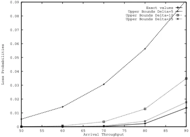
the packet size is 512 bytes. We plot the loss probabilities of the rightmost queue for input bit rate varying from 50 Mb/s to 90 Mb/s. In Fig.2, we consider three queues in tandem, with the same capacity, equal to 20. The size of the exact Markov process is 9261. We can see the results of upper bounds of loss probabilities according to different values of ∆ ( 5,10, 15) for respective aggregated Markov processes sizes ( 4231, 6951, 8631). We can notice that more ∆ increases and the better is the bounds since it approaches the exact values. In Fig. 3, we consider four queues in tandem, with the same capacity, equal to 20.The size of the exact Markov process is 194481 and we take different values of ∆ ( 5,10, 15) for respective
aggregated Markov processes sizes (50781 ,158071, 191751). We can also notice that more ∆ increases and the better is the bounds since it approaches the exact values. Note that we have proposed in this paper a particular aggregation scheme, others must be tried in order to see the impact on the quality of the bounds. 0.3 0.35 0.4 0.45 0.5 50 55 60 65 70 75 80 85 90 Loss Probabilities Arrival Throughput Exact Upper Bounds Delta=5 upper Bounds Delta=10 upper Bounds Delta=15
Fig. 2. Three queues in tandem : exact and upper bounds loss probabilities
0 0.01 0.02 0.03 0.04 0.05 0.06 0.07 0.08 0.09 50 55 60 65 70 75 80 85 90 Loss Probabilities Arrival Throughput Exact values Upper Bounds Delta=5 Upper Bounds Delta=10 Upper Bounds Delta=15
Fig. 3. Four queues in tandem : exact and upper bounds loss probabilities
VI. CONCLUSION
We apply stochastic comparison method in order to reduce the size of large state Markov processes. We present an algorithm which generates for a given large Markov process, the aggregated Markov process which provides bounds on performance measures. This algorithm has been applied to the analysis of tandem queues. Loss probabilities bounds have been computed and prove that the methodology is interesting. Different aggregation schemes can be performed by the pro-posed algorithm since the constraints on the aggregated states are not very restrictive. Thus we can have a tradeoff between the accuracy of bounds and the computation complexity. Furthermore, the proposed approach can be also applied to provide transient bounds.
APPENDIX
Stochastic comparison method is based on the stochastic ordering theory. Two formalisms can be used : increasing functions [11], [5] or increasing sets [8] . The ¹st is the most
known stochastic ordering and it is equivalent to the sample path ordering (see Strassen’s theorem [11]). Let E be a discrete and countable state space, and ¹ be at least a preorder (reflex-ive, transitive but not necessarily anti-symmetric) on E. We
consider two random variables X and Y defined respectively on E, and their probability measures given respectively by the probability vectors p and q where p[i] = P rob(X = i), ∀i ∈
E (resp. q[i] = P rob(Y = i), ∀i ∈ E).
Definition 1: X ¹st Y ⇔ E[(f (X))] ¹ E[(f (Y ))] ∀f :
E → R, ¹-increasing whenever the expectations exist.
Different formalisms can be used for the ”¹st” ordering : the
coupling [11], [6], or the increasing set theory [8] which is presented in the sequel.
Let Γ ⊆ E, we denote by Γ ↑= {y ∈ E | y º x, x ∈ Γ}. Definition 2: Γ is called an increasing set if and only if Γ = Γ ↑.
The ¹stordering can also be defined using the increasing set
theory [8] : Definition 3: X ¹st Y ⇔ p ¹st q ⇔ p(Γ) ≤ q(Γ), ∀Γ²Φst(E), where p(Γ) = P x∈Γ p[x]
Where Φst(E) is the family of increasing sets which induces
the ”¹st” ordering : Φst(E) = {all increasing sets on E}
We explain now the stochastic comparison of Markov processes. We suppose the general case where they are not defined on the same state space, and we map them into a common state space in order to compare them. The stochastic comparison of Markov processes by mappings is used in this paper in order to reduce the state space of the Markov process. Let {X(t), t ≥ 0} (resp. {Y (t), t ≥ 0}) a Markov process defined on E (resp. F ), with infinitesimal generator matrix Q1 (resp. Q2). We define by g a many to one mapping from E to
S, and h a many to one mapping from F to S. We compare
stochastically the image g(X(t)) of X(t) with h(Y (t)) of
Y (t).
Definition 4: We say that {g(X(t)), t ≥ 0} ¹st
{h(Y (t)), t ≥ 0} if g(X(0)) ¹st h(Y (0)) =⇒ g(X(t)) ¹st
h(Y (t)), ∀t > 0
Mapping functions can be represented by matrices. Let Mg
(resp. Mh) denotes the matrix representing the mapping g
(resp. h).
Mg[i, j]i∈E andj∈S=
½
1 if g(i) = j 0 else
and similarly, Mh is defined by replacing g by h, and E by
F . We give the theorem of the stochastic comparison using
increasing set theory [8] :
Theorem 1: If the following conditions 1, 2 and 3 are satisfied : 1) g(X(0)) ¹sth(Y (0)) 2) {g(X(t)), t ≥ 0} or {h(Y (t)), t ≥ 0} is ¹st-monotone 3) Q1[x, ∗]Mg ¹st Q2[y, ∗]Mh, ∀x ∈ E, y ∈ F, g(x) = h(y) then {g(X(t)), t ≥ 0} ¹st{h(Y (t)), t ≥ 0} where Q1[x, ∗]Mg ¹st Q2[y, ∗]Mh ⇔ P g(z)∈ΓQ1(x, z) ≤ P h(z)∈ΓQ2(y, z), ∀Γ ∈ Φst(S), ∀x ∈ E, y ∈ F | g(x) = h(y).
The monotonicity of the Markov process is used in condition (2) of this theorem, it is defined as an increasing of the process in t [6] :
Definition 5: We say that {X(t), t ≥ 0} is ¹st -monotone
if X(t) ¹stX(t + τ ), ∀t ≥ 0, τ > 0;
To establish the monotonicity of a process {X(t), t ≥ 0}, we can use the coupling of the processes [6], [7]. Let
b
X(t), cX0(t) two processes governed by the same infinitesimal
generator matrix than {X(t), t ≥ 0}, representing different realizations of {X(t), t ≥ 0} with different initial conditions.
The theorem of the monotonicity using the coupling states as follows [6], [7]:
Theorem 2: We say that {X(t), t ≥ 0} is ¹st -monotone if
and only if there exists the coupling {( bX(t), cX0(t)), t ≥ 0} such that bX(0) ¹ cX0(0) ⇒ bX(t) ¹ cX0(t), ∀t > 0
This theorem can be proved [6], by verifying that coupling conditions on the infinitesimal generator hold. When we study the mapping of a process, we can also define the monotonicity, and it is formulated as follows [11], [6]:
Definition 6: We say that {f (X(t)), t ≥ 0} is ¹st
-monotone if f (X(s)) ¹stf (X(t)), ∀s, t ∈ R+, s ≤ t The increasing set formalism can be used to formulate the monotonicity of the mapping of a Markov process [11], [6].
Theorem 3: We say that {f (X(t)), t ≥ 0} is
¹st -monotone if and only if: Q1[x, ∗]Mf ¹st
Q1[y, ∗]Mf, ∀x, y ∈ E | f (x) ¹ f (y)
Next, we give the general algorithm of the aggregation of Markov processes, in order to derive performance measures bounds.
REFERENCES
[1] J.Ben Othman, H.Castel(Taleb), L.Mokdad, ”Multi-services MAC proto-col for wireless networks”, the third ACS/IEEE International Conference in Computer Systems and Applications, CAIRO 3-6 January 2005 [2] H.Castel, L. Mokdad, ”Performance measure bounds in wireless networks
by state space reduction”, 13th Annual Meeting of the IEEE Interna-tional Symposium on Modeling, Analysis, and Simulation of Computer and Telecommunication Systems (MASCOTS 2005), 27-29 september, Atlanta Georgia.
[3] H.Castel, L. Mokdad, N .Pekergin, ”Loss rates bounds for IP switches in MPLS networks”, ACS/IEEE International Conference on Computer Systems and Applications AICCSA-06, 8-11 March 2006, Dubai/Sharjah, UAE.
[4] H. Castel, J.M. Fourneau, N. Pekergin, ”Stochastic bounds on partial ordering: application to memory overflows due to bursty arrivals”, 20th International Symposium on Computer and Information Sciences (ISCIS 2005), October 26-28 2005, Istanbul, Turkey, published in LNCS by Springer-Verlag.
[5] M.Doisy, ”Comparaison de processus Markoviens”, PHD thesis, Univ. de Pau et des pays de l’Adour 92.
[6] T.Lindvall, ”Lectures on the coupling method”, Wiley series in Probability and Mathematical statistics, 1992.
[7] T. Lindvall, ”Stochastic monotonicities in Jackson queueing networks”, Prob. in the Engineering and Informational Sciences 11, 1997, 1-9. [8] W. Massey, ”Stochastic orderings for Markov processes on partially
ordered spaces” Mathematics of Operations Research, Vol.12, N2, May 1987.
[9] H.G. Perros, ”Queueing networks with blocking, exact and approximate solutions”, Oxford university press, 1994.
[10] N. Pekergin, ”Stochastic performance bounds by state space reduction”, Performance evaluation, 36-37, (1-17), 1999.
[11] D. Stoyan, ”Comparison methods for queues and other stochastics models”, J. Wiley and son, 1976.
[12] L. Zheng, L. Zhang, ”Modeling and performance analysis for IP traffic with multi-class QoS in VPN”, Milcom2000, 21st Century Military Communications Conference Proceedings, Vol 1, 22-25 Oct. Page 330-334, vol1.