Harry Zekollari1,2,3,4, Matthias Huss1,2,5, and Daniel Farinotti1,2
1Laboratory of Hydraulics, Hydrology and Glaciology (VAW), ETH Zürich, Zürich, Switzerland,2Swiss Federal Institute for Forest, Snow and Landscape Research (WSL), Birmensdorf, Switzerland,3Department of Geoscience and Remote Sensing, Delft University of Technology, Delft, Netherlands,4Laboratoire de Glaciologie, Université libre de Bruxelles, Brussels, Belgium,5Department of Geosciences, University of Fribourg, Fribourg, Switzerland
Abstract
Glaciers in the European Alps rapidly lose mass to adapt to changes in climate conditions. Here, we investigate the relationship and lag between climate forcing and geometric glacier response with a regional glacier evolution model accounting for ice dynamics. The volume loss occurring as a result of the glacier‐climate imbalance increased over the early 21st century, from about 35% in 2001 to 44% in 2010. This committed loss reduced to ~40% by 2018, indicating that temperature increase was outweighing glacier retreat in the early 2000s but that the fast retreat effectively somewhat diminished glacierimbalances. We analyze the lag in glacier response for each individual glacier andfind mean response times of 50 ± 28 years. Ourfindings indicate that the response time is primarily controlled by glacier slope and secondarily by elevation range and mass balance gradient, rather than by glacier size.
Plain Language Summary
Glaciers are out of balance with present‐day climatic conditions. By using a state‐of‐the‐art computer model that can simulate the evolution of many glaciers, we show that the imbalance between glaciers in the European Alps and climatic conditions grew during the early 21st century. Although this imbalance has recently decreased, glaciers are still expected to lose an important part of their mass, even if temperatures were to be stabilized at present‐day levels. This is an expression of glaciers adapting to present‐day climatic conditions. Our simulations suggest that the glacier response is strongly dependent on the surface steepness rather than on glacier size, as commonly reported.1. Introduction
Glaciers have globally been losing mass at an accelerated pace over the past few decades (Wouters et al., 2019; Zemp et al., 2019). This is also the case in the European Alps (Berthier et al., 2016; Dehecq et al., 2016; Fischer et al., 2015), where glaciers have been subject to strongly negative mass balances (e.g., Charalampidis et al., 2018; Thibert et al., 2018; Vincent et al., 2018; Zekollari & Huybrechts, 2018). By retreating, glaciers lose ice at their lower elevations, which has a stabilizing feedback on their mass balance, hence reducing the imbalance between glacier geometry and the climatic conditions (hereafter referred to as “glacier‐climate imbalance”). At the same time, further temperature increase (e.g., Rottler et al., 2019) causes a decrease in the glacier mass balance, thereby increasing the glacier‐climate imbalance. The mass balance of a glacier, thus, reflects the interplay between changes in glacier geometry and changes in climate conditions. Due to the lag between climatic forcing and glacier response, however, solely relying on the mass balance does not give a clear indication of the dominating process (supporting information, Figure S1). The use of mass balance as a metric for the glacier‐climate imbalance is furthermore complicated by the fact that by losing mass, the glacier does not only reduce its area but also thins, which further decreases the local mass balance (Huss et al., 2012). An alternative and more complete approach for quantifying the evolution of the glacier‐climate imbalance consists of quantifying the dynamic response of glaciers (e.g., Christian et al., 2018). Recent efforts in this direction have been undertaken by Marzeion et al. (2018), who utilized a simple glacier evolution model based on volume scaling to analyze the present‐day committed glacier loss at the global scale.
Here, we use a novel glacier evolution model (Zekollari et al., 2019) that explicitly accounts for surface mass balance (SMB) and iceflow processes, to quantify the temporal evolution of the committed glacier loss in the European Alps. Through various numerical experiments, we aim at shedding light on the evolution of the
©2020. The Authors.
This is an open access article under the terms of the Creative Commons Attribution License, which permits use, distribution and reproduction in any medium, provided the original work is properly cited.
Key Points:
• Climate warming outpaced glacier retreat in the European Alps until 2010, increasing the imbalance between glacier geometry and climate
• After 2010, the imbalance between glacier geometry and climate decreased, but a committed volume loss of ~40% is still projected • First regional glacier response time
inventory accounting for iceflow, hinting at the crucial role of the glacier slope, as opposed to size
Supporting Information: • Supporting Information S1 Correspondence to: H. Zekollari, h.zekollari@tudelft.nl Citation:
Zekollari, H., Huss, M., & Farinotti, D. (2020). On the Imbalance and Response Time of Glaciers in the European Alps.
Geophysical Research Letters, 47, e2019GL085578. https://doi.org/ 10.1029/2019GL085578
Received 26 SEP 2019 Accepted 6 JAN 2020
glacier‐climate imbalance over time and its link to the glacier response time. The glacier response time of Alpine glaciers has typically been studied for single or a few glaciers (e.g., Le Meur & Vincent, 2003; Oerlemans, 2007, 2012; Zekollari & Huybrechts, 2015) or through simplified approaches in which ice dynamics were not explicitly included (e.g., Haeberli & Hoelzle, 1995; Raper & Braithwaite, 2009). Here, we complement these efforts by deriving thefirst regional‐scale glacier response time inventory with a physically based model and determine the main factors that control the response time of individual glaciers.
2. Materials and Methods
The temporal glacier evolution is simulated with GloGEMflow (Zekollari et al., 2019), which is an extended version of the Global Glacier Evolution Model (GloGEM, Huss & Hock, 2015) incorporating ice dynamics. For this study, we do not consider glaciers shorter than 1 km, as these small ice bodies have a very limited mass transfer through ice dynamics and can quickly disintegrate under changing climatic conditions (Huss & Fischer, 2016), which cannot accurately be captured with a large‐scale flowline model. The 795 glaciers longer than 1 km represent ~95% of the total volume and 86% of the total area of all glaciers in the European Alps (Zekollari et al., 2019). For every individual glacier, a calibration is performed to match the glacier length and volume at the Randolph Glacier Inventory (RGI, RGI Consortium, 2017) date (typically 2003). The calibration procedure starts from a 1990 steady‐state glacier by perturbing the mean 1961–1990 climatology and adjusts for a factor describing the ice flow in order to match the geometry at the inventory date (seefigure 3 in Zekollari et al., 2019). We do not explicitly account for thermodynamics and rely on the commonly used approximation in which all ice is considered to be temperate (e.g., Le Meur et al., 2004; Schmeits & Oerlemans, 1997). GloGEMflow and its calibration procedure were extensively evaluated over Alpine glaciers by comparing, among others, modelled and observed SMBs (WGMS, 2018), surface velocities (e.g., Berthier & Vincent, 2012), and recent glacier changes (GLAMOS, 2018a). The future glacier evolution modelled with GloGEMflow, moreover, was shown to agree well with results from detailed studies that used 3‐D higher‐order and full‐Stokes models for individual glaciers (e.g., Jouvet et al., 2011; Jouvet & Huss, 2019; Zekollari et al., 2014).
3. Data
The model calibration, detailed in Zekollari et al. (2019), is based on the glacier geometry and outlines from the RGI v6.0 (RGI Consortium, 2017). Ice thickness is derived following the method of Huss and Farinotti (2012), as provided within the consensus estimate by Farinotti et al. (2019), with a mean uncertainty on the volume of individual glaciers of about 20%. The SMB model was calibrated to reproduce the geodetic mass balances of individual glaciers, which were taken from the World Glacier Monitoring Service database (WGMS, 2018). The climatic data used to force the SMB model comes from the ENSEMBLES daily gridded observational dataset (E‐OBS; Cornes et al., 2018). These data are downscaled to individual glaciers as part of the calibration procedure to reproduce the geodetic mass balance of individual glaciers (see Huss & Hock, 2015).
4. Glacier‐Climate Imbalance
The recent evolution of the imbalance between the glacier geometry and the climate is investigated through transient simulations in which the ice loss that would occur if the climate was to remain constant (section 4.1) is analyzed. These simulations are complemented with experiments assessing the temporal evolution of the forcing needed to preserve the volume and length of Alpine glaciers at a given point in time (section 4.2).
4.1. Committed Loss
For every given year between 2001 and 2018, the committed loss is derived by constantly forcing the glacier model with the mean SMB of the previous 30 years and by running the glaciers to steady state under these conditions (Figure 1a). The SMB is calculated for a reference geometry and is subsequently expressed as a local function of elevation. As the geometry evolves, the SMB for every altitude is then determined by inter-polating the elevation‐dependent SMB to the considered elevation.
The committed loss experiments indicate that the committed loss increased in the early 21st century (in both relative and absolute terms, see Figure 1b), suggesting that the glaciers' capability of adapting their geometry
10.1029/2019GL085578
through retreat was outpaced by rising temperatures. In 2001, the committed volume loss (under 1972–2001 mean SMB) was 42 km3or 34% of the total ice volume at that time (125 km3). In 2010, the committed loss increased to 45 km3or 42%, from 107 km3in 2010 to 62 km3at steady state. The committed loss stabilized and decreased after ca. 2010 (Figure 1b), suggesting that glacier retreat outpaced the warming over the last decade, thus reducing the glacier‐climate imbalance. In general, the relative committed ice loss is larger for small glaciers than it is for large ones (see Figure S2 and Table S1, where uncertainty is also addressed).
4.2. Conservation Experiments
As an alternative metric characterizing the glacier‐climate imbalance, we analyze which climatic forcing would be needed at any point in time to preserve on the one hand the total glacier volume and on the other hand the cumulative length of all glaciers in the European Alps. For this, we rely on the same setting as for the committed loss experiments (section 4.1) and apply a temperature anomaly on top of that. Experiments with different temperature anomalies suggest that for maintaining the total volume in 2001 (~125 km3, Figures 2a and 2b), a temperature forcing of−0.65 °C (compared to 1972–2001) would have been needed. For 2010 (total volume≈107 km3, Figures 2a and 2c), thisfigure changes to −0.75 °C; that is, actual tempera-tures were three quarters of degree warmer than what would have permitted glacier balance. These values are in line with thefindings from the committed loss experiments, suggesting that warming dominated over glacier geometric adaptations during thefirst decade of the 21st century. After 2010, the trend is reversed and the glacier‐climate imbalance reduces. Since 2010, mean annual temperatures increased by about 0.2 °C (derived from E‐OBS over glacierized areas, considering 30‐year means), while the imbalance (i.e., the tem-perature forcing needed to maintain the volume) decreased by ~0.1 °C (Figures 2a and 2d). By conceptually expressing the imbalance change as the sum of the temperature change and the geometric adaptation, a geometric adaptation corresponding to 0.3 °C is obtained over this period. This is 50% more important than the actually realized temperature change. Similarfindings are obtained when considering precipitation, where a forcing of +21%, +25%, and +18% is needed in 2001, 2009, and 2019, respectively (Figure S3). In the volume conservation experiments, the total volume remains relatively stable over time (Figures 2b–2d). However, the spatial volume distribution in the final steady state is different than in the transient case, with usually slightly shorter glaciers (Figures S4a and S4c). The frontal regions of the steady‐state glaciers are generally also thicker and steeper than transient glaciers with same volume. This is because the local flux divergence has to compensate the very negative SMB at low elevations (see Figures S4a and S4c; Zekollari & Huybrechts, 2015). In general, large steady‐state glaciers tend to have a slightly lower volume than their transient counterparts, which is an expression of large glaciers being
Figure 1. Committed glacier volume evolution for the European Alps between 2001 and 2018. The committed evolution at any given time is defined as the volume
trajectory occurring when imposing the mean SMB conditions of the previous 30 years. (a) Evolution of volume over time. The black line is the actual glacier evolution between 1990 and 2018 (modelled by Zekollari et al., 2019), while the colored lines indicate the committed evolution. (b) Relative (dark grey) and absolute (light grey) committed volume loss for a given year. The dashed lines correspond to a second‐order polynomial fit.
proportionally more out of balance (i.e., more negative SMB) compared to small glaciers. The differences are, however, generally small. For instance, glaciers with a present‐day volume of more than 1 km3 have a steady‐state volume that is 1.4% smaller on average than their transient counterpart (for the volume conservation experiment in 2011).
In order to preserve the glacier area or length at a given moment in time, a more pronounced forcing (varying between−0.95 and −0.75 °C; see Figures 2e–2g) is needed for the length conservation experiments compared to the volume conservation experiments. This results in steady‐state glaciers with a larger volume than the transient case (up to 10% larger ice volume, Figures 2b–2g). These experiments illustrate the slow response of Alpine glaciers: Even for cases where a negative temperature forcing is imposed to maintain the total glacier length on the longer run (i.e., when considering steady state), a strong initial decline in glacier length occurs. For the length conservation experiments starting around 2010 (when the climate‐geometry imbalance is the largest), glaciers lose about 12–13% of their total length over 30 years (Figure 2f), before eventually re‐advancing and recovering the initial length. These simulations require temperature adjustments of up to−0.95 °C, and the mass excess at low elevation is first removed (thus causing glacier retreat; Figures S4a, S4b, and S4d) before being replaced by the additional mass added at higher elevations (thus causing re‐advance, Figures S4a and S4e). The slow response also appears from the SMB evolution, which initially increases and becomes positive (Figures 2h–2j) as a reaction to glacier retreat. As glaciers re‐advance, the SMB decreases and eventually evolves to zero when the glaciers reach a steady state. Both the committed and volume conservation experiments suggest that glacier retreat started to catch up and outpace the climatic warming signal around 2010. This is in agreement withfield observations, which
Figure 2. (a) Temperature anomaly needed at any given point in time to maintain the total glacier volume at that time.
The black circles indicate the temperature forcing needed to maintain the volume in 2001, 2011, and 2018 (panels b–j). Evolution of glacier volume (b–d), glacier length (e–g), and glacier‐wide mass balance (h–j) for conservation experiments starting in 2001, 2011, and 2018. The values are integrated over all glaciers of the European Alps.
10.1029/2019GL085578
indicate several record‐breaking years of volume loss and glacier retreat after 2010 (2011, 2012, 2015, 2017, and 2018; GLAMOS, 2018b). The timing of the shift in the glacier‐climate imbalance may partially be explained by the fact that around the late 1980s, many Alpine glaciers where relatively close to equilibrium. The subsequent rise in temperatures caused glaciers to thin, but due to the glacier response time, it took yet another 20–30 years for glacier retreat and frontal loss to peak.
5. Response Time
5.1. Response Time of the Entire Alpine Ice Mass
The glacier response time from numerical experiments can be expressed through an e‐folding timescale, in which the response time corresponds to the time needed to complete 1− e−1(= 63.2%) of the total change (e.g., Leysinger Vieli & Gudmundsson, 2004; Oerlemans, 2018). For the committed experiments (Figure 2), the above approach results in response times decreasing from 42 years in 2001 to 33 years in 2018 (Figure S5). This decrease may reflect changing geometric conditions, but its interpretation is compli-cated by the transient signal of ongoing retreat interfering with the response to the imposed climatic conditions (see, e.g., Zekollari & Huybrechts, 2015, for a more detailed discussion). Furthermore, in these committed experiments, the individual glaciers will have an integrated mass balance which may strongly vary: For a given scenario, some glaciers may strongly retreat, while others will change only little or even advance.
In order to isolate the effect of the transient glacier evolution and to ensure that glaciers are subject to the same forcing, additional simulations are performed in which steady‐state glaciers are taken as a starting point and are continuously forced until a new steady state is reached. For this, spatially homogeneous
Figure 3. Response time experiments from simulations in which every glacier is subject to the same temperature forcing. (a) Evolution of the total ice volume of all
glaciers in the European Alps. The eight lines depict the different experiments in which the glaciers are forced to evolve from one steady state to another by applying temperature perturbations compared to the 1972–2001 reference period (purple) and the 1989–2018 reference period (green). (b) e‐folding response times of the entire Alpine ice mass (τalps) derived from simulations presented in panel (a). Modelled response time of individual glaciers (τglac) as a function of surface slope along the (c)flowline and (d) glacier area. The correlation is significant at 1% and 5% significance level when R2> 0.09 and R2> 0.07, respectively.
climatic perturbations are considered, allowing us to directly compare the response time between glaciers. Two glacier advance simulations (evolution from steady state with temperature forcing of (i) 0 to−1 °C and (ii)−0.5 to −1 °C) and two glacier retreat simulations (evolution from steady state with temperature forcing of (i)−1 to 0 °C and (ii) −0.5 to 0 °C) are performed for two distinct reference periods (1972–2001 and 1989–2018, respectively; Figure 3a). In these eight experiments, steady‐state glaciers are created that are slightly smaller, similar in size, and slightly larger than present‐day glaciers (Figure 3a).
These simulations indicate that the response time of the entire Alpine ice mass varies between 36 and 78 years (Figure 3b). The lower end of this range, between 36 and 45 years (Figure 3b), corresponds to strong retreat experiments and is in line with the response times derived from the transient simulations (33–42 years, Figure S5). The longer response times (55 years and more) correspond to the advance cases, where the imposed, additional accumulation needsfirst to travel through the glacier before resulting in an actual glacier advance.
5.2. Response Time of Individual Glaciers
The numerical simulations allow us to quantify the response time of every individual glacier. For glaciers longer than 1 km at inventory date, a mean response time of 50 ± 28 years is obtained (mean over all glaciers and the eight experiments presented in section 5.1 ± one standard deviation; for uncertainty, refer to Table S1). Similar mean response times are obtained when weighing by glacier area (49 ± 28 years) or glacier volume (54 ± 28 years), hinting at a limited link between glacier response time and glacier size. To gain insights into the drivers of glacier response time, a total of 18 predictors describing various glacier character-istic are used in a set of regression analyses (see Figures S6 and S7). These predictors, of which many are correlated, are subdivided into three main categories characterizing (i) glacier size (e.g., glacier volume, area, and length), (ii) glacier slope along theflowline (various slope quantiles), and (iii) glacier SMB (frontal SMB, equilibrium line altitude, and SMB gradient).
In a regression analysis with only one predictor variable, the surface slope along theflowline explains most of the inter‐glacier variability in response time: 39% and 42% for linear and quadratic regressions, respec-tively (Figure 3c). Considering the surface slope over a lower fraction of the glacier (e.g., Brun et al., 2019; Fischer et al., 2015; Huss & Fischer, 2016) does not improve this correlation significantly (Figures S6, S7, and S8a). The correlation between the response time and size‐dependent variables is insignificant (Figure S6 and S7). Glacier area, for example, yields R2< 0.01 (Figure 3d). An exception is the elevation range (R2= 0.23 and 0.31 for linear and quadratic regression, respectively), which is itself linked to the surface slope. The frontal SMB and the SMB gradient in the ablation area describe a small fraction of the response time (for quadratic regression: R2= 0.15 and 0.19, respectively; p < 0.01; Figure S6). Increasing the order of the polynomialfit to 3 or 4 has only a limited effect (Figure S7).
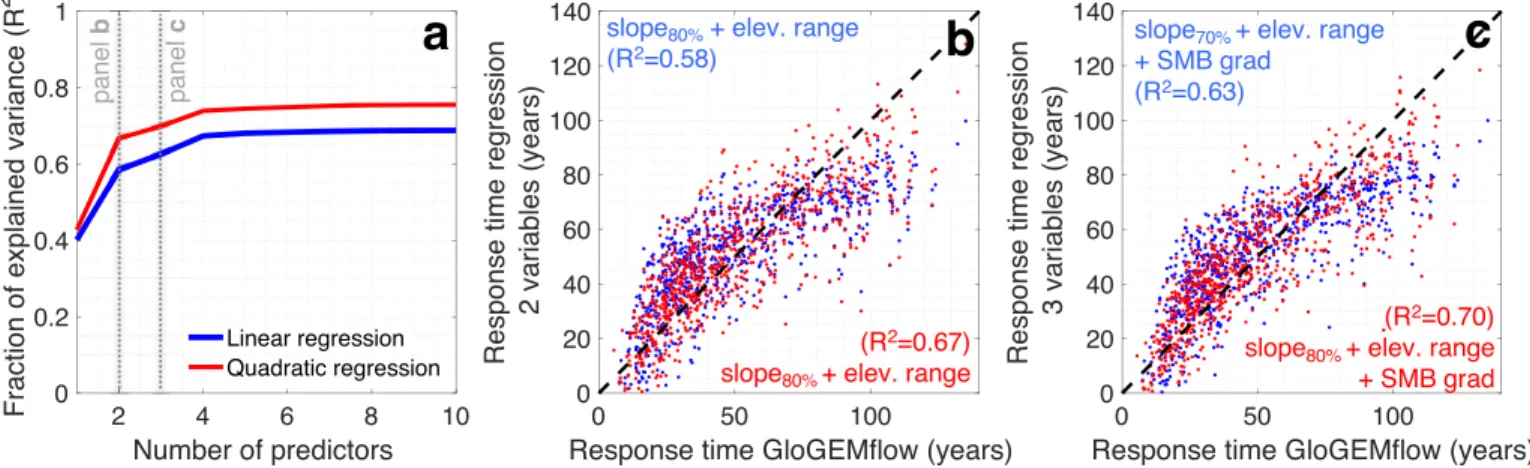
By combining two predictor variables (ignoring interaction terms), more than two thirds of the variability in response time can be described: Together, (i) the surface slope along theflowline of the lowest 80% of the elevation range and (ii) the elevation range explain up to 67% of the variance (quadratic regression; Figure 4b). In general, most of the variability is explained when combining (i) a variable related to the glacier slope with (ii) a variable related to the SMB (Figure S9a). With three predictors, the highest portions of explained variance (up to 70% for quadratic regression) are obtained when combining a slope‐, a size‐, and an SMB‐related variable (Figures 4c and S9b). When considering four predictors, up to 74% of the variance can be explained (Figures S8b and S9c), indicating a saturation of the explanatory power provided by adding further predictors (Figure 4a).
The surface slope is the main driver for the response time and is in all cases negatively correlated with the latter (Figures 3c and S6): Steeper glaciers are able to efficiently transfer mass and adapt rapidly and thus have shorter response times (e.g., Haeberli & Hoelzle, 1995; Oerlemans, 2012). Glaciers with a steeper SMB gradient—those tending to have a more negative frontal SMB—are able to react faster and have shorter response times (Figure S6). This is in line with widely used analytical response time expressions (e.g., Harrison et al., 2001; Jóhannesson et al., 1989), in which the frontal SMB is in the denominator. For glaciers in the European Alps, this lower frontal SMB counters—and in some cases even outweighs—the higher ice thickness (numerator in the response time definition by Jóhannesson et al., 1989) as glacier size grows (Bahr et al., 1998; Oerlemans, 2012; Raper & Braithwaite, 2009). As a result, the effect of glacier size on the
10.1029/2019GL085578
response time is very weak to inexistent (Figure S6) and only appears for size‐related variables that are correlated to the frontal SMB (e.g., highest elevation or elevation range). Our numerical simulations thus suggest that recurring statements linking glacier response time to size (e.g.,“larger glaciers have a longer response time”) are not valid for glaciers in the European Alps longer than 1 km. For glaciers outside the European Alps, the relationship between glacier size and response time may change as a result of the climatic conditions, larger elevation ranges, and/or other mechanisms. In cold and dry regions, large glaciers often cover the landscape and the increase in glacier size leads to a strong decrease in surface slope. This may result in a positive correlation between glacier size and response time. On the contrary, in maritime regions, the glacier size is strongly dependent on the magnitude of the SMB gradient and may thus negatively correlate with response time.
Our analysis indicates that nearby glaciers of similar size may have substantially different response times. This difference can help explaining why some similarly sized neighboring glaciers have very distinct mass balances. Our results thus complement studies investigating mass balance variability (e.g., Brun et al., 2019; Fischer et al., 2015) and sensitivity (e.g., Huss & Fischer, 2016), which also found that surface slope is a main driver of inter‐glacier SMB variability at the local scale.
6. Conclusions
Through numerical simulations of glacier evolution, we showed that glaciers in the European Alps are to lose a substantial part of their mass under present‐day climatic conditions. The mass loss committed from this imbalance increased during thefirst decade of the 21st century and slightly decreased after 2010. At pre-sent, the committed mass loss amounts to ~40% of the present‐day ice volume. The lag between climatic for-cing and glacier adaptation is directly related to the glacier response time, which is on average 50 ± 28 years for glaciers in the European Alps longer than 1 km. At the individual glacier level, we showed that this response time is mainly related to the glacier slope. SMB and size‐related characteristics such as glacier area and volume only play a secondary role. Our results indicate that 58% of the variance between the response times of individual glaciers longer than 1 km within the European Alps can be explained with the following relation:
τ ¼ 121−1:24·α80%−0:028 Δz;
whereτ (years) is the glacier response time; α80% (%) is the average surface slope along the flowline of the lowest 80% of elevation of the glacier, andΔz (m) is the glacier's elevation range. This can be used as a rule of thumb to estimate the response time of an Alpine glacier without any numerical modelling. The relation can be extended with additional predictors and a quadraticfit to explain up to three quarters of the inter‐ glacier response time variability.
Figure 4. (a) Fraction of response time variability explained with multilinear (blue) and quadratic (red) regression when considering a given number of predictors.
Relation between response time derived from numerical GloGEMflow simulations (x axis) and from regression analysis (y axis) when using (b) two or (c) three predictors. The blue (red) dots and equations represent the linear (quadratic) regression.
This is thefirst study to investigate glacier response times at a regional scale with an ice dynamical model and opens the door to global‐scale response‐time studies encompassing glacier types featuring additional processes such as calving or supraglacial debris coverage, which can introduce additional feedback mechan-isms. Such studies may hold the key for better understanding local‐ to regional‐scale differences in glacier responses to a changing climate.
References
Bahr, D. B., Pfeffer, W. T., Sassolas, C., & Meier, M. F. (1998). Response times of glaciers as a function of size and mass balance: 1. Theory.
Journal of Geophysical Research, 103(B5), 9777–9782. https://doi.org/doi:10.1029/98JB00507
Berthier, E., Cabot, V., Vincent, C., & Six, D. (2016). Decadal region‐wide and glacier‐wide mass balances derived from multi‐temporal ASTER satellite digital elevation models. Validation over the Mont‐Blanc Area. Frontiers in Earth Science, 4, 63. https://doi.org/10.3389/ feart.2016.00063
Berthier, E., & Vincent, C. (2012). Relative contribution of surface mass‐balance and ice‐flux changes to the accelerated thinning of Mer de Glace, French Alps, over 1979–2008. Journal of Glaciology, 58(209), 501–512. https://doi.org/10.3189/2012JoG11J083
Brun, F., Wagnon, P., Berthier, E., Jomelli, V., Maharjan, S. B., Shrestha, F., & Kraaijenbrink, P. D. A. (2019). Heterogeneous influence of glacier morphology on the mass balance variability in High Mountain Asia. Journal of Geophysical Research: Surface, 124, 1–15. https:// doi.org/10.1029/2018JF004838
Charalampidis, C., Fischer, A., Kuhn, M., Lambrecht, A., Mayer, C., Thomaidis, K., & Weber, M. (2018). Mass‐budget anomalies and geometry signals of three Austrian glaciers. Frontiers in Earth Science, 6, 218. https://doi.org/10.3389/feart.2018.00218
Christian, J. E., Koutnik, M., & Roe, G. (2018). Committed retreat: Controls on glacier disequilibrium in a warming climate. Journal of
Glaciology, 64, 675–688. https://doi.org/10.1017/jog.2018.57
Cornes, R. C., van der Schrier, G., van den Besselaar, E. J. M., & Jones, P. D. (2018). An ensemble version of the E‐OBS temperature and precipitation data sets. Journal of Geophysical Research Atmospheres, 123, 9391–9409. https://doi.org/10.1029/2017JD028200 Dehecq, A., Millan, R., Berthier, E., Gourmelen, N., Trouv, E., & Vionnet, V. (2016). Elevation changes inferred from TanDEM‐x data over
the Mont‐Blanc area impact of the X‐band interferometric bias. IEEE Journal of Selected Topics in Applied Earth Observations and
Remote Sensing, 9(8), 3870–3882.
Farinotti, D., Huss, M., Fürst, J. J., Landmann, J., Machguth, H., Maussion, F., & Pandit, A. (2019). A consensus estimate for the ice thickness distribution of all glaciers on Earth. Nature Geoscience., 12(3), 168–173. https://doi.org/10.1038/s41561‐019‐0300‐3 Fischer, M., Huss, M., & Hoelzle, M. (2015). Surface elevation and mass changes of all Swiss glaciers 1980–2010. The Cryosphere, 9(2),
525–540. https://doi.org/10.5194/tc‐9‐525‐2015
GLAMOS. (2018a). Swiss glacier length change, release 2018, Glacier Monitoring Switzerland. https://doi.org/10.18750/length-change.2018.r2018.
GLAMOS. (2018b). Swiss glacier mass balance, release 2018, Glacier Monitoring Switzerland. https://doi.org/10.18750/massbalance.2018. r2018.
Haeberli, W., & Hoelzle, M. (1995). Application of inventory data for estimating characteristics of and regional climate‐change effects on mountain glaciers: A pilot study with the European Alps. Annals of Glaciology, 21, 206–212. https://doi.org/10.3189/ S0260305500015834
Harrison, W. D., Elsberg, D. H., Echelmeyer, K. A., & Krimmel, R. M. (2001). On the characterization of glacier response by a single time‐ scale. Journal of Glaciology, 47(159), 659–664.
Huss, M., & Farinotti, D. (2012). Distributed ice thickness and volume of all glaciers around the globe. Journal of Geophysical Research, 117, F04010. https://doi.org/10.1029/2012JF002523
Huss, M., & Fischer, M. (2016). Sensitivity of very small glaciers in the Swiss Alps to future climate change. Frontiers in Earth Science, 4, 1–17. https://doi.org/10.3389/feart.2016.00034
Huss, M., & Hock, R. (2015). A new model for global glacier change and sea‐level rise. Frontiers in Earth Science, 3, 1–22. https://doi.org/ 10.3389/feart.2015.00054
Huss, M., Hock, R., Bauder, A., & Funk, M. (2012). Conventional versus reference‐surface mass balance. Journal of Glaciology, 58(208), 278–286. https://doi.org/10.3189/2012JoG11J216
Jóhannesson, T., Raymond, C. F., & Waddington, E. D. (1989). A simple method for determining the response time of glaciers. In Glacier
Fluctuations and Climatic Change(pp. 343–352). Dordrecht: Kluwer Academic Publishers.
Jouvet, G., & Huss, M. (2019). Future retreat of Great Aletschgletscher. Journal of Glaciology, 65(253), 869–872. https://doi.org/10.1017/ jog.2019.52
Jouvet, G., Huss, M., Funk, M., & Blatter, H. (2011). Modelling the retreat of Grosser Aletschgletscher, Switzerland, in a changing climate.
Journal of Glaciology, 57(206), 1033–1045. https://doi.org/10.3189/002214311798843359
Le Meur, E., Gagliardini, O., Zwinger, T., & Ruokolainen, J. (2004). Glacierflow modelling: A comparison of the Shallow Ice Approximation and the full‐Stokes solution. Comptes Rendus Physique, 5(7), 709–722. https://doi.org/10.1016/j.crhy.2004.10.001 Le Meur, E., & Vincent, C. (2003). A two‐dimensional shallow ice‐flow model of Glacier de Saint‐Sorlin, France. Journal of Glaciology,
49(167), 527–538. https://doi.org/10.3189/172756503781830421
Leysinger Vieli, G. J.‐M. C., & Gudmundsson, G. H. (2004). On estimating length fluctuations of glaciers caused by changes in climatic forcing. Journal of Geophysical Research, 109, F01007. https://doi.org/10.1029/2003JF000027
Marzeion, B., Kaser, G., Maussion, F., & Champollion, N. (2018). Limited influence of climate change mitigation on short‐term glacier mass loss. Nature Climate Change, 8(4), 305–308. https://doi.org/10.1038/s41558‐018‐0093‐1
Oerlemans, J. (2007). Estimating response times of Vadret da Morteratsch, Vadret da Palü, Briksdalsbreen and Nigardsbreen from their length records. Journal of Glaciology, 53(182), 357–362. https://doi.org/10.3189/002214307783258387
Oerlemans, J. (2012). Linear modelling of glacier lengthfluctuations. Geografiska Annaler, Series A: Physical Geography, 94(2), 183–194. https://doi.org/10.1111/j.1468‐0459.2012.00469.x
Oerlemans, J. (2018). Modelling the late‐Holocene and future evolution of Monacobreen, northern Spitsbergen. The Cryosphere, 12, 3001–3015. https://doi.org/10.5194/tc‐12‐3001‐2018
Raper, S. C., & Braithwaite, R. J. (2009). Glacier volume response time and its links to climate and topography based on a conceptual model of glacier hypsometry. The Cryosphere, 3, 183–194. https://doi.org/10.5194/tcd‐3‐243‐2009
10.1029/2019GL085578
Geophysical Research Letters
Acknowledgments
H. Zekollari acknowledges the funding received from WSL's Internal Innovative
Projectsscheme, the Swiss Federal Office for the Environment Hydro‐
CH2018project, and a Marie Skłodowska‐Curie Individual Fellowship (Grant 799904). We thank the data providers in the ECA&D project (http://www.ecad.eu), which contributed to the E‐OBS dataset. We are very grateful for the thoughtful and constructive reviews by two anonymous reviewers,which were of great help to improve the paper. The response time of every individual glacier is available in the online research data repository of ETH Zürich (https://www.research‐ collection.ethz.ch/handle/ 20.500.11850/388137).
RGI Consortium. (2017). Randolph Glacier Inventory—A dataset of global glacier outlines: Version 6.0: Technical report, Global Land Ice Measurements from Space, Colorado, USA. Digital Media. https://doi.org/10.7265/N5‐RGI‐60
Rottler, E., Kormann, C., Francke, T., & Bronstert, A. (2019). Elevation‐dependent warming in the Swiss Alps 1981–2017: Features, forcings and feedbacks. International Journal of Climatology, 39(5), 2556–2568. https://doi.org/10.1002/joc.5970
Schmeits, M. J., & Oerlemans, J. (1997). Simulation of the historical variations in length of Unterer Grindelwaldgletscher, Switzerland.
Journal of Glaciology, 43(143), 152–164.
Thibert, E., Sielenou, P. D., Vionnet, V., Eckert, N., & Vincent, C. (2018). Causes of glacier melt extremes in the Alps since 1949. Geophysical
Research Letters, 45, 817–825. https://doi.org/10.1002/2017GL076333
Vincent, C., Soruco, A., Azam, M. F., Basantes‐Serrano, R., Jackson, M., Kjøllmoen, B., et al. (2018). A nonlinear statistical model for extracting a climatic signal from glacier mass balance measurements. Journal of Geophysical Research: Earth Surface, 123, 2228–2242. https://doi.org/10.1029/2018JF004702
WGMS. (2018). Fluctuations of glaciers database. World Glacier Monitoring Service, Zurich, Switzerland. https://doi.org/10.5904/wgms‐ fog‐2018‐06.
Wouters, B., Gardner, A. S., & Moholdt, G. (2019). Global glacier mass loss during the GRACE satellite mission (2002–2016). Frontiers in
Earth Science, 7, 96. https://doi.org/10.3389/feart.2019.00096
Zekollari, H., Fürst, J. J., & Huybrechts, P. (2014). Modelling the evolution of Vadret da Morteratsch, Switzerland, since the Little Ice Age and into the future. Journal of Glaciology, 60(224), 1208–1220. https://doi.org/10.3189/2014JoG14J053
Zekollari, H., Huss, M., & Farinotti, D. (2019). Modelling the future evolution of glaciers in the European Alps under the EURO‐CORDEX RCM ensemble. The Cryosphere, 13, 1125–1146. https://doi.org/10.5194/tc‐13‐1125‐2019
Zekollari, H., & Huybrechts, P. (2015). On the climate–geometry imbalance, response time and volume–area scaling of an alpine glacier: Insights from a 3‐D flow model applied to Vadret da Morteratsch, Switzerland. Annals of Glaciology, 56(70), 51–62. https://doi.org/ 10.3189/2015AoG70A921
Zekollari, H., & Huybrechts, P. (2018). Statistical modelling of the surface mass balance variability of the Morteratsch glacier, Switzerland: Strong control of early melting season meteorological conditions. Journal of Glaciology, 64(244), 275–288. https://doi.org/10.1017/ jog.2018.18
Zemp, M., Huss, M., Thibert, E., Eckert, N., McNabb, R., Huber, J., et al. (2019). Global glacier mass balances and their contributions to sea‐level rise from 1961 to 2016. Nature, 568(7752), 382–386. https://doi.org/10.1038/s41586‐019‐1071‐0