HAL Id: hal-01069708
https://hal.archives-ouvertes.fr/hal-01069708
Submitted on 29 Sep 2014
HAL is a multi-disciplinary open access
archive for the deposit and dissemination of
sci-entific research documents, whether they are
pub-lished or not. The documents may come from
teaching and research institutions in France or
abroad, or from public or private research centers.
L’archive ouverte pluridisciplinaire HAL, est
destinée au dépôt et à la diffusion de documents
scientifiques de niveau recherche, publiés ou non,
émanant des établissements d’enseignement et de
recherche français ou étrangers, des laboratoires
publics ou privés.
Thermal effects on solar images recorded in space
Abdanour Irbah, Mustapha Meftah, Alain Hauchecorne, Luc Damé, Maxime
Bocquier, Momar Cissé
To cite this version:
Abdanour Irbah, Mustapha Meftah, Alain Hauchecorne, Luc Damé, Maxime Bocquier, et al..
Ther-mal effects on solar images recorded in space. Proc. SPIE 9143, Space Telescopes and
Instru-mentation 2014: Optical, Infrared, and Millimeter Wave, Jun 2014, Montréal, Canada. pp.914342,
�10.1117/12.2054741�. �hal-01069708�
Thermal e
ffects on solar images recorded in Space
Irbah A.
a, Meftah M.
a, Hauchecorne A.
a, Dam´e L.
a,
Bocquier M.
aand Ciss´e M.
aa
LATMOS - Laboratoire Atmosph`
eres, Milieux, Observations Spatiales, CNRS : UMR8190
-Universit´
e Paris VI - Pierre et Marie Curie - Universit´
e de Versailles
Saint-Quentin-en-Yvelines - INSU 78280, Guyancourt, France
ABSTRACT
The Earth’s atmosphere introduces a spatial frequency filtering in the object images recorded with ground-based instruments. A solution is to observe with telescopes onboard satellites to avoid atmospheric effects and to obtain diffraction limited images. However, similar atmosphere problems encountered with ground-based instruments may subsist in space when we observe the Sun since thermal gradients at the front of the instrument affect the observations. We present in this paper some simulations showing how solar images recorded in a telescope focal plane are directly impacted by thermal gradients in its pupil plane. We then compare the results with real solar images recorded with the PICARD mission in space.
Keywords: Satellite, Solar diameter, Space observations
1. INTRODUCTION
The Earth atmosphere limits high resolution observations performed with ground-based instruments. Indeed, the Earth atmosphere is a turbulent media that affects the light-of-sight when observing the object of interest with ground-based instruments. Consequences are a spatiotemporal filtering of high frequencies of the recorded images. A solution to avoid these problems is to observe in orbit on satellite platforms. Instruments in orbit are however submitted to others constraints due to the space environment. In this case, the Earth atmosphere is generally not in the light-of-sight when observing objects but space-based telescopes receive others radiation flux incoming directly from the Earth (long-wave radiations) or after reflections of solar radiations on the upper layers of the Earth atmosphere (short-wave radiations). These flux have effects on the telescope pupil that perturb the observations as when observing from ground. In addition, the observations are more sensitive to the thermal gradients at the front of the instrument when we observe the Sun. We present in this paper some simulations showing how solar images recorded in the telescope focal plane are impacted by thermal gradients present at the front of the instrument. We then use the simulation results to interpret what we observe from the solar images recorded with the SODISM (Solar Diameter Imager and Surface Mapper) of the PICARD space mission.
2. THE PICARD MISSION : OBJECTIVES AND DIFFICULTIES
First, we give a brief description of the PICARD mission and its telescope SODISM. Then, we present the problems encountered when the observations were analyzed.
2.1 The PICARD telescope
The PICARD solar mission was launched on June 15, 2010 and has observed until April 2014. Its main objectives were the measurements of the diameter and the asphericity of the Sun at several wavelengths (215, 393.37, 535.7, 607.1 and 782.2 nm), the limb shape at the same wavelengths, the differential rotation, the Total Solar Irradiance (TSI), the Spectral Solar Irradiance (SSI) in UV, visible and IR, and to get images for helioseismologic studies to probe the inner Sun. The PICARD mission operates during the rising phase of the solar cycle 24 allowing to study the variation of these quantities with the solar activity. The satellite is in a Sun synchronous Orbit with
Further author information:
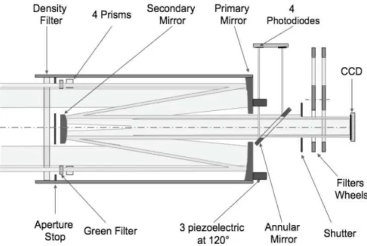
Figure 1. SODISM optical scheme.
an ascending node at 06h00, an orbit inclination of 98 degrees, an altitude of 730 km and a period of about 100 minutes. Annual eclipses exist in such orbits, but they last for 20 minutes maximum (for instance in December). The total PICARD payload weight is about 125 kg. It includes absolute radiometers and photometers for the TSI and SSI measurements and SODISM, an imaging telescope developed to measure the diameter, the limb shape and the asphericity of the Sun. A detailed description of the PICARD telescope may be found in Meftah et al. (2014).7 We recall here some of its main properties. The optical scheme of SODISM which is a Ritchey-Chr´etien telescope, is shown in Figure 1. SODISM images the whole solar disk on a CCD (Charge-Coupled Device) sensor. A window (density filter in Figure 1) is set in front of the telescope to limit the solar energy to 5% of the total solar irradiance. The pupil diameter of the telescope is 8.9 cm. The wavelengths are selected by interference filters on 2 wheels. Wavelength domains are chosen free of Fraunhofer lines (535.7, 607.1 and 782.2 nm). Active regions are detected in the 215 nm domain and the CaII (393.37 nm) line. Helioseismologic observations are performed at 535.7 nm.2 The spacecraft pointing is stabilized to better than 36 arc-seconds. The telescope primary mirror stabilizes the solar image within 0.2 arc-second, using a proper piezo-electric system. An internal calibration system is used to determine scale factor variations induced by instrument deformations, which result from temperature fluctuations in orbit or others causes.1, 5 The diameter measurements are referred to star angular distances by rotating the spacecraft towards some doublet stars several times a year. The instrument stability is ensured by the use of stable materials (Zerodur for mirrors, Carbon-Carbon and Invar for structure). The whole instrument temperature is stabilized within 1o
C, the CCD around −7o
C within 0.2o C.
2.2 The PICARD observations and lessons
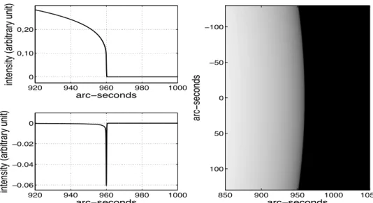
The PICARD telescope records full and limb images of the Sun at all the wavelengths mentioned above. Full resolution solar images are 2048x2048 pixels size. The pixel size was estimated in space using the Venus transit, which occurred in June, 2012. It is equal to 1.064 arc-seconds.8 Limb images corresponding to 22 or 40 pixels wide limbs6are obtained by masking the solar image to take only the pixels where the limb is imaged on the camera. The Figure 2(a) shows a full solar image recorded at 607.1 nm on July 22, 2010 16:11 UT. The Figure 2(b) plots a solar limb extracted from the image while Figure 2(c) represents its gradient. The solar limb is the variation of the Sun intensity around one radius. The width of the solar limb gradient is directly related to the point spread function (psf ) of the telescope since the true solar limb is not resolved by the instrument.4 The width of this solar limb gradient taken at 2/3 of its extremum is found equal to 3.1 arc-seconds which is greater than the expected value for the wavelength 617.1 nm and a telescope pupil of 8.9 cm. Several fits of simulated limb gradients based on a theoretical limb model (see section 3.2) and a perfect telescope with different pupil diameter sizes are plotted in Figure 2(d). We found that the observed limb corresponds to a telescope pupil diameter of 4 cm revealing that SODISM was defocused. We will use this value in the following for our study.
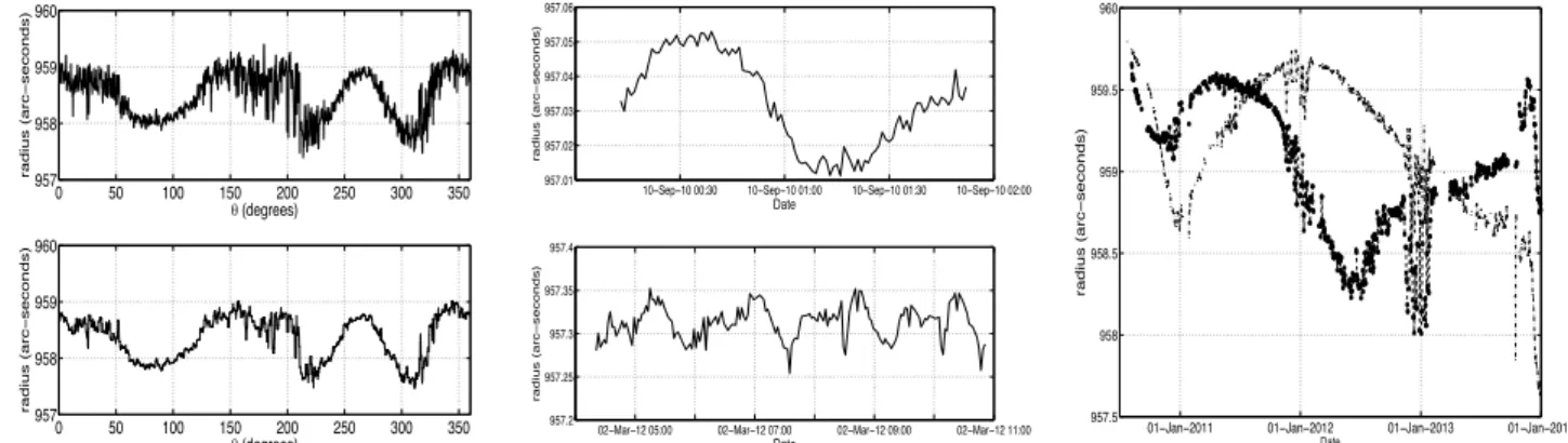
The PICARD astrometry program needs to extract the solar shape defined as the position of the inflection point of a radial solar limb in all azimuthal angles from 0 to 360 degrees. The upper curve of the Figure 3 left panel
(a) 8000 850 900 950 1000 1050 1100 0.5 1 1.5 2 2.5x 10 4
intensity (arbitrary unit)
r (arc−seconds) (b) 900 920 940 960 980 1000 −1 −0.8 −0.6 −0.4 −0.2 0 r (arc−seconds)
normalized intensity (arbitrary unit)
(c) 900 920 940 960 980 1000 −1 −0.8 −0.6 −0.4 −0.2 0 r (arc−seconds)
normalized intensity (arbitrary unit)
(d)
Figure 2. (a) Solar image recorded with SODISM at 607.1 nm on July 22, 2010 16:11. (b) Extracted limb from the image and its derivative (c). (d) plots the limb derivative fitted by a model (see text).
plots the solar edge extracted from a SODSIM image recorded on October 1, 2011 at 535.7 nm while the lower one shows the same solar edge after some filtering that reveal strong discontinuities together with angular radius variations due to the telescope optical response. The solar radius extracted from each recorded image is then the angular mean value of the solar shape corrected from the satellite-Sun distance. The Figure 3 middle panel plots the mean solar radius obtained from image series recorded at 535.7 nm on September 10, 2011 during one orbit (upper curve) and at 607.1 nm on March 2, 2012 during 4 orbits (lower curve). Orbital signatures are clearly observed in the solar radius measurements. The Figure 3 right panel plots the daily mean solar radius obtained at 535.7 nm and 607.1 nm with PICARD during the whole mission. The eclipse periods i.e. the Earth is in the line of sight during the observations, are clearly recognizable by the important fluctuations in the measurements. We see clearly that they are some variations in the solar radius greater than one arc-second that could not be attributed to the Sun. We propose in the following section, to provide partial explanations to these unexpected observable. 0 50 100 150 200 250 300 350 957 958 959 960 θ (degrees) radius (arc − seconds) 0 50 100 150 200 250 300 350 957 958 959 960 θ (degrees) radius (arc − seconds)
10−Sep−10 00:30 10−Sep−10 01:00 10−Sep−10 01:30 10−Sep−10 02:00
957.01 957.02 957.03 957.04 957.05 957.06 Date radius (arc − seconds)
02−Mar−12 05:00 02−Mar−12 07:00 02−Mar−12 09:00 02−Mar−12 11:00
957.2 957.25 957.3 957.35 957.4 Date radius (arc − seconds)
01−Jan−2011 01−Jan−2012 01−Jan−2013 01−Jan−2014
957.5 958 958.5 959 959.5 960 Date radius (arc − seconds)
Figure 3. Solar shape extracted from the image recorded at 535.7 nm on October 1, 2011 with SODISM (left panel). Short (middle panel) and long-time (right panel) solar radius variations obtained with SODISM at 535 nm (*) and 607 nm (.).
3. THERMAL EFFECTS ON THE FRONT WINDOWS. SIMULATION OF IMAGE
DEGRADATIONS
We suppose that the temperature variations in the PICARD front windows may explain parts of the problems encountered in the observation analysis. They are responsible of the wavefront degradations incoming from the Sun. Indeed, the entrance window of the SODISM telescope is composed with silica suprasil material, which has a low coefficient of thermal expansion but has high refractive index variations with the temperature.
3.1 The optical model
The refractive index dependence with the temperature T (r, z) in the filter density is expressed as:
n(r, T (r, z)) = n0+ ∆nT×(T (r, z) − T0) (1)
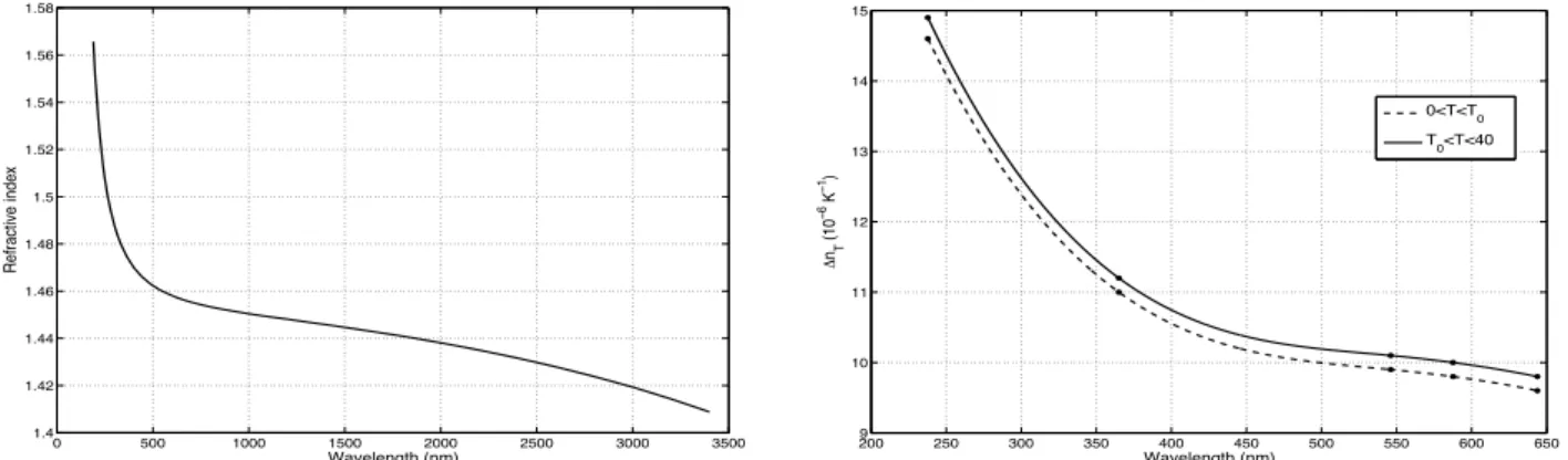
where r = r(x, y) and z are the point coordinates in the density filter. ∆nT and n0 are obtained for a given wavelength from Figure 4.10 These curves are valid for ground experiments at T
0 = 20 o
C and 1 bar (values given by the manufacturer10
) but the difference is small for space ones.
The wavefront degradations are due to the path-length difference δ(r) at each point resulting from its propagation through the front windows. It is given by:
δ(r) = !
h
n(r, T (r, z))dz (2)
where h is the thickness of the density filter equal to 8 mm.
The instrument is seen as having a pupil function P (r) with aberrations due to the thermal effects in the front windows:
P (r) = P0×exp iΦ(r) (3)
where
Φ(r) = 2π
λδ(r) (4)
is the perturbed wavefront and P0the pupil function with no aberrations defined as: P0(r) =
"
1 si r <= D/2
0 otherwise (5)
with D = 114mm, the diameter of the density filter.
The psf of the perturbed instrument is then obtained taking the power spectrum of P (r) given by Equation 3. It will be used to build solar images in different cases of temperature configuration maps in the front windows.
0 500 1000 1500 2000 2500 3000 3500 1.4 1.42 1.44 1.46 1.48 1.5 1.52 1.54 1.56 1.58 Wavelength (nm) Refractive index 2009 250 300 350 400 450 500 550 600 650 10 11 12 13 14 15 Wavelength (nm) Δ nT (10 − 6 K − 1) 0<T<T 0 T0<T<40
Figure 4. The left panel shows the wavelength dependence of the refractive index of suprasil glass at T0 = 20 o
C and 1 bar.10
diameter (m) tickness (m) (a) −0.04 −0.03 −0.02 −0.01 0 0.01 0.02 0.03 0.04 2 4 6 8 x 10⁻³ 19 20 21 22 23 24 25 diameter (m) tickness (m) (b) −0.04 −0.03 −0.02 −0.01 0 0.01 0.02 0.03 0.04 2 4 6 8 x 10⁻³ 1.4578 1.4578 1.4578 1.4578 1.4578 1.4578 1.4578 −0.05 −0.04 −0.03 −0.02 −0.01 0 0.01 0.02 0.03 0.04 0.05 0.0102 0.0102 0.0102 0.0102 0.0102 0.0102 0.0102 diameter (m) δ(r) (mm)
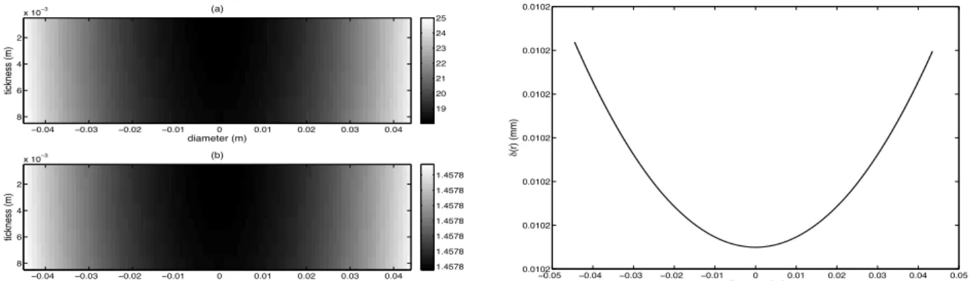
Figure 5. The left panel shows the cross-section maps of the three-dimensional simulation temperature (a) and of the refractive index (b). The corresponding path-length difference δ(r) is plotted in the left panel.
3.2 Simulations of
psf ’s and degraded solar images
We suppose in a first approach that a great part of the observed effects in the SODISM focal plane are explained by a defocus induced by the temperature gradient variations occurring along the orbit. A defocused wavefront can be described by a path-length difference δ(r) = a×(r − r0)2 where 1/a and r0 are respectively the curvature radius and the extremum position of the parabolic wavefront. The phase of the defocused wavefront Φ(r) is related to the path-length difference δ(r) by Equation 4. The Peak to Valley (P-V) wavefront error i.e. the deviation of the perturbed wavefront to a reference surface, is generally given using the wavelength λ as unit. The path-length difference in wavelength unit considering that δ(D/2) = xλ where x is a real, is then written:
δ(r) = 4
(D − 2r0)2
×(r − r0)2×(xλ) = δ(x, r) (6)
We use Equation 6 in the simulation to create wavefronts with different perturbations thanks to the x parameter. We need first a temperature map of the front windows. A previous work shows that the center of the density filter is cooler that the border.7 The temperature is around 15o
C in the center while it is 28o
C at the border giving rise to a radial gradient. We create a parabolic function for the temperature centered on the density filter i.e. r0 = 0 and having these values in all its radial cuts. The generated temperature map has then an axial symmetry. The temperatures inside the density filter are obtained by interpolation. This interpolation is performed by taking radial cuts of the density filter following its thickness. Figure 5(a) shows a cross-section map of the three-dimensional simulation temperature T (r, z) for the wavelength 607.1 nm. We use it to compute the associated refractive index map n(r, T ) thanks to Equation 1 and the path-length difference δ(r) (see Figure 5 right panel) allowing deducing the perturbed wavefront Φ(r). We use it to build the psf and consequently the degraded solar images. Figure 6 shows a psf obtained with no degradation (left panel) and with 2 λ P-V phase errors (right panel). An image representing the true Sun is necessary for our needs and thus a limb model to build the simulated images. The solar limb darkening function at the extremely solar edge is computed with
arc−seconds arc − seconds −60 −40 −20 0 20 40 60 −60 −40 −20 0 20 40 60 arc−seconds arc − seconds −60 −40 −20 0 20 40 60 −60 −40 −20 0 20 40 60
920 940 960 980 1000 0
0,10 0,20
arc−seconds
intensity (arbitrary unit)
920 940 960 980 1000 −0.06 −0.04 −0.02 0 arc−seconds
intensity (arbitrary unit)
arc−seconds arc − seconds 850 900 950 1000 1050 −100 −50 0 50 100
Figure 7. Theoretical limb (top left panel), its derivative (bottom left panel) and the simulated solar image (right panel)
a numerical model developed by N. Mein9 while another model is used for the center to limb intensity.3 This combined model (see top of Figure 7 left panel) allows then to build the useful Sun image. The bottom of Figure 7 left panel plots the derivative of the solar combined model where we see that the limb spreads over only few hundreds of milliarcseconds. This means that the extreme solar limb is not resolved by the instrument SODISM, which has a resolution of about one arc-second. We have then a possibility to study the behavior of the instrument by observing the solar limb gradient as already done for the atmospheric turbulence.4 The Figure 7 left panel shows the simulated Sun image computed over a field a little more higher than 200 arc-seconds side. The degraded image corresponding to the psf of Figure 6 has been computed (see Figure 8 left panel). It is the result of the convolution between the Sun image and the psf. We see also in Figure 8 right panel a degraded solar limb (top) and its derivative (bottom) extracted from the image as well as the corresponding theoretical
arc−seconds arc − seconds 850 900 950 1000 1050 −100 −50 0 50 100 920 940 960 980 1000 0 0,20 0,40 0,60 arc−seconds
intensity (arbitrary unit)
920 940 960 980 1000 −0.06 −0.04 −0.02 0 arc−seconds
intensity (arbitrary unit)
Figure 8. Simulation of a degraded solar image (left panel), an extracted limb and its derivative (respectively top and bottom right panel).
150 160 170 180 190 200 210 220 230 240 250 0 0.1 0.2 0.3 0.4 0.5 0.6 arc−seconds
intensity (arbitrary unit)
(a) 0.4λ 0.9λ 1.3λ 1.6λ 2λ 150 160 170 180 190 200 210 220 230 240 250 0 0.1 0.2 0.3 0.4 0.5 0.6 arc−seconds
intensity (arbitrary unit)
(b) 0.4λ 0.9λ 1.3λ 1.6λ 2λ 150 160 170 180 190 200 210 220 230 240 250 −4 −3.5 −3 −2.5 −2 −1.5 −1 −0.5 0x 10 −3 arc−seconds
intensity (arbitrary unit)
(c) 0.4λ 0.9λ 1.3λ 1.6λ 2λ 150 160 170 180 190 200 210 220 230 240 250 −5 −4.5 −4 −3.5 −3 −2.5 −2 −1.5 −1 −0.5 0x 10 −3 arc−seconds
intensity (arbitrary unit)
(d) 0.4λ 0.9λ 1.3λ 1.6λ 2λ
Figure 9. Solar limb at 535.7 nm (a) and 607.1 nm (b) in different degradation cases. (c) and (d) are their derivative. ones (dashed line curves). The degradation effects are clearly visible on the derivative of the solar limb and this has consequences when analyzing the PICARD images.
4. APPLICATIONS TO PICARD OBSERVATIONS
We present first in this section how wavefront degradations associated to the image analysis method affect the results. We will limit our study to the PICARD wavelength 535.7 and 607.1 nm.
4.1 Degradations consequences for the image analysis
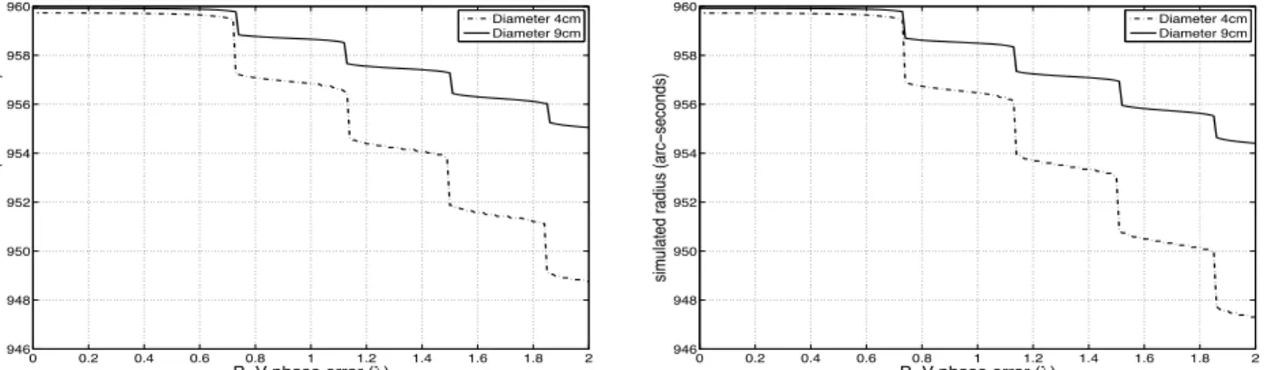
The temperature map of the instrument front windows evolves continually along the satellite orbit and when the Earth moves on its trajectory around the Sun. This will have an impact on the image degradations as seen in the previous section. We have simulated solar images in various P-V phase errors and observed the effects on the solar limb. We consider first the temperature map centered on the telescope optical axis (r0 = 0). Figure 9(a) and (b) plot the degraded solar limbs extracted for images computed at 535.7 and 607.1 nm for x = 0.4 to x = 2 (see Equation 6). As expected, we see clearly that the limb spread out as the x parameter increases. This is best observed in their derivative where we notice also that the side lobes increase (see Figure 9(c) and (d)). This x parameter effect will have then important consequences on the solar radius estimated from the inflection point position of the limb i.e. the extremum of its derivative. Figure 10 plots the solar radius obtained from these images where the Sun model image had an arbitrary value at 960 arc-seconds. We observe for both wavelengths that there is a decrease of the solar radius with the x parameter but also some gaps occurring when the side lobes have values greater than the main one. These curves have been computed for a pupil diameter of the instrument of 9 cm (quasi perfect SODISM instrument) and 4 cm since we noticed in Section 2.2 that the recorded limbs at the beginning of the mission corresponded to this equivalent pupil. We see also in the figure that the x parameter effect on the solar radius is greater for smaller pupil diameters. The consequence of shifted temperature maps
0 0.2 0.4 0.6 0.8 1 1.2 1.4 1.6 1.8 2 946 948 950 952 954 956 958 960 P−V phase error (λ)
simulated radius (arc
− seconds) Diameter 4cm Diameter 9cm 0 0.2 0.4 0.6 0.8 1 1.2 1.4 1.6 1.8 2 946 948 950 952 954 956 958 960 P−V phase error (λ)
simulated radius (arc
−
seconds)
Diameter 4cm Diameter 9cm
Figure 10. Reduction of solar radius at 535.7 nm (left panel) and 607.1 nm (right panel) with the P-V phase error for a pupil diameter of 4 and 9 cm
0 0.5 1 1.5 935 940 945 950 955 960 P−V phase error (λ)
simulated radius (arc
− seconds) r0=0.00 cm r0=0.25 cm r 0=0.50 cm r 0=0.75 cm r 0=1.00 cm r 0=1.25 cm r 0=1.50 cm 0 0.5 1 1.5 935 940 945 950 955 960 P−V phase error (λ)
simulated radius (arc
− seconds) r0=0.00 cm r0=0.25 cm r 0=0.50 cm r 0=0.75 cm r 0=1.00 cm r 0=1.25 cm r 0=1.50 cm
Figure 11. Reduction of solar radius at 535.7 nm (left panel) and 607.1 nm (right panel) with the P-V phase error for a pupil diameter of 4 cm. The temperature map is shifted relatively to the optical axis from r0= 0 to r0= 1.5 cm.
relatively to the instrument optical axis (r0 parameter) is shown in Figure 11 for both wavelengths and for a pupil diameter of 4 cm. We notice that the decrease of the radius is greater when r0 increases but the radius gaps remain at the same x values. The curve we consider for our PICARD data analysis will be chosen such as all the radius measurements of the mission are on the same curve part without gaps as confirmed by the Figure 3 right panel. The curve corresponding to r0= 0.75 cm will be chosen in the following.
4.2 Analysis of the PICARD results
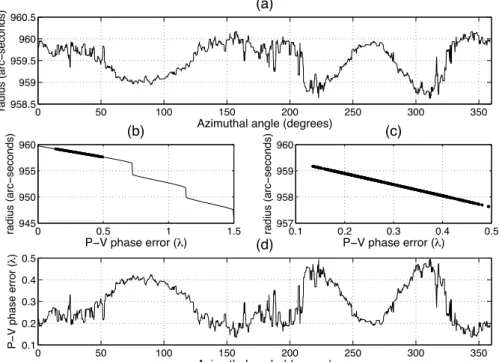
We use the simulations results presented in the previous section to interpret what is observed in the PICARD data analysis. We consider first the solar shape in Figure 12(a) recorded on October 1, 2011 at 535.7 nm and the curve of Figure 11 left panel that gives the radius behavior with the x parameter. All the radius values are plotted on this curve (Figure 12(b) and (c)). We observe a good relationship between the model obtained from the simulations and the PICARD data. A three-order polynomial function is found as a good approximation
0 50 100 150 200 250 300 350 958.5 959 959.5 960 960.5
Azimuthal angle (degrees)
radius (arc − seconds) (a) 0 50 100 150 200 250 300 350 0.1 0.2 0.3 0.4 0.5
Azimuthal angle (degrees)
P − V phase error ( λ ) (d) 0 0.5 1 1.5 945 950 955 960 P−V phase error (λ) radius (arc − seconds) (b) 0.1 0.2 0.3 0.4 0.5 957 958 959 960 P−V phase error (λ) (c) radius (arc − seconds)
10−Sep−10 00:30 10−Sep−10 01:00 10−Sep−10 01:30 10−Sep−10 02:00 957 957.01 957.02 957.03 957.04 957.05 957.06 Date radius (arc − seconds)
02−Mar−12 05:00 02−Mar−12 07:00 02−Mar−12 09:00 02−Mar−12 11:00
957.2 957.25 957.3 957.35 957.4 Date radius (arc − seconds)
10−Sep−10 00:30 10−Sep−10 01:00 10−Sep−10 01:30 10−Sep−10 02:00
957 957.01 957.02 957.03 957.04 957.05 957.06 Date radius (arc − seconds)
02−Mar−12 05:00 02−Mar−12 07:00 02−Mar−12 09:00 02−Mar−12 11:00
957.2 957.25 957.3 957.35 957.4 Date radius (arc − seconds)
10−Sep−10 00:30 10−Sep−10 01:00 10−Sep−10 01:30 10−Sep−10 02:00
0.618 0.62 0.622 0.624 0.626 0.628 Date P − V phase error ( λ )
02−Mar−12 05:00 02−Mar−12 07:00 02−Mar−12 09:00 02−Mar−12 11:00
0.495 0.5 0.505 0.51 Date P − V phase error ( λ )
Figure 13. The left panel plots the fit of the temporal solar radius measurements at 535.7 (top,line) and 607.1 nm (bottom,line) with our gradient model (dot). The temporal radius variations are fitted with a sum of 2 sin functions (middle panel) leading to estimate the gradients causing them with our model (right panel)
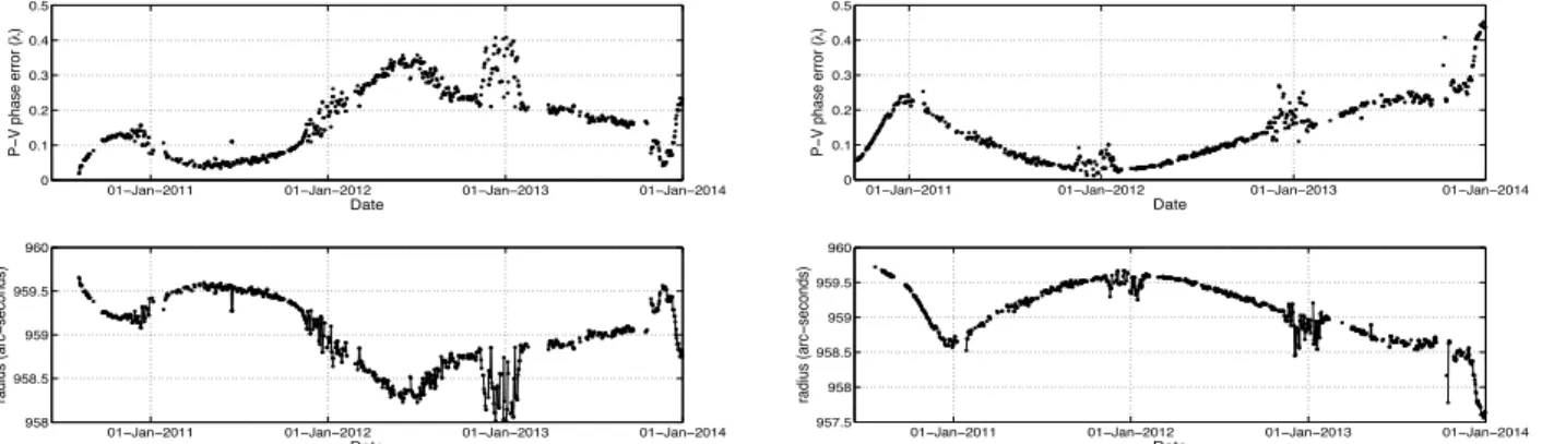
of the model i.e. ∆(R) ∝ (x3) where ∆(R) is the radius variations and ∝ denotes the proportionality factor. We use this function to estimate the angular gradients at the front of the instrument that are responsible of the limb degradations (Figure 12(d)). The same model is applied to fit the solar radius recorded during few orbits. The obtained gradients allow to fit correctly the data (see Figure 13 left panel). The temporal variations of the solar radius is also well approximated by the sum of two Sin functions of period 50 ± 3 and 100 ± 3 minutes, the last one being that of PICARD (see middle panel of Figure 13). We use this approximation with our model and obtain the same results for the gradients (see right panel of Figure 13). Finally the same work is performed on the radius data of all the PICARD mission. The top of Figure 14 plots the obtained gradients that fits the solar radius shown on the bottom in the same figure. We observe that we have similar amplitudes of the gradient variations during all the measurement period for both wavelength but they are not in phase. We note also that the amplitude of the radius variations observed on the solar shape and during the mission correspond to x parameter variation of the same order. If we consider for example the wavelength 535.7 nm, the solar shape has a variation of 1.54 arc-seconds peak-to-peak which corresponds to a x parameter variation of 0.36 (see Figure 12) while it is 1.65 arc-seconds for the mission solar radius corresponding to 0.39 x parameter variation (see Figure 13). The same remark is valid for the wavelength 607.1 nm. The solar radius variations are then due to the P-V phase error fluctuations. We need however to improve our model to explain the spectral phase shift by adding some other hypothesis than only the defocus of the images due to thermal gradients in the front windows.
01−Jan−2011 01−Jan−2012 01−Jan−2013 01−Jan−2014
0 0.1 0.2 0.3 0.4 0.5 Date P− V phase error ( λ )
01−Jan−2011 01−Jan−2012 01−Jan−2013 01−Jan−2014
958 958.5 959 959.5 960 Date radius (arc − seconds)
01−Jan−2011 01−Jan−2012 01−Jan−2013 01−Jan−2014
0 0.1 0.2 0.3 0.4 0.5 Date P− V phase error ( λ )
01−Jan−2011 01−Jan−2012 01−Jan−2013 01−Jan−2014
957.5 958 958.5 959 959.5 960 Date radius (arc − seconds)
Figure 14. Temporal gradient estimated to fit the temporal solar radius at 535.7 nm (left panel) and 607.1 nm (right panel)
5. CONCLUSION
PICARD is a space solar mission launched on June 15, 2010 and ended on April 2014. Among its objectives, there is an astrometry program which include the measurement of solar radius and its temporal variations. The data analysis of PICARD revealed however some unexpected observable such as (i) a spread of the solar limb at the beginning of the mission larger than expected, (ii) solar shapes extracted from the images presenting strong discontinuities and (iii) important variations of short and long-term solar radius not directly attributed to the Sun’s physics. We have then developed in this paper a simple model to explain parts of these observables since a previous work shown that radial thermal gradients exist in the front windows of the PICARD telescope. This model suppose that these thermal gradients introduce a defocus of the recorded images, which evolves in time as the satellite rotates around the Earth and the Earth around the Sun. Perturbed wavefronts have been simulated based on the thermal properties of the front window. They were used to simulate in a first step psf in various P-V phase errors and then solar images as formed with the PICARD telescope. We use for that a Sun image built on a theoretical model of the solar limb darkening function and having a constant solar radius of 960 arc-seconds. The analysis of the simulated images allowed us to find a relationship between the obtained solar radius and the P-V phase errors. The results revealed also that measured solar radius obtained from the inflection point positions of the solar limb presented some gaps for some particular values of the P-V phase errors. Our model allowed us to estimate the thermal gradients in the front window that explain the observed solar radius variations shown in PICARD data analysis. We conclude that the solar radius variations are directly related to the variations of the P-V phase errors. However considering 2 different wavelength (535.7 and 607.1 nm), we noticed that the gradients are of the same order but have a temporal shift although images are recorded at the quasi same time on the orbit. We still need to improve our model to explain this spectral temporal shift by adding some other hypothesis than only the image defocus.
ACKNOWLEDGMENTS
This work has been supported by CNRS and the Centre National d’Etudes Spatiales (France).
REFERENCES
[1] Assus, P., Irbah, A., Bourget, P., Corbard, T. & the PICARD team, 2008, Astron. Nachr., 329, 5, 517 [2] Corbard, T., Salabert, D., Boumier, P., Appourchaux, T., Hauchecorne, A. et al, 2013, Journal of Physics:
Conference Series, 440, 012025
[3] Hestroffer, D., Magnan, C., and Loeser, R., 1998, Astronomy and Astrophysics, v.333, p.338-342
[4] A. Irbah, J. Borgnino, F. Laclare, and G. Merlin, “Isoplanatism and high spatial resolution solar imaging,” Astron. Astrophys., 276, pp. 663–672, 1993.
[5] Irbah, A., Meftah, M., Hauchecorne, A., Cisse, M & Rouze, M., 2012, Proceedings SPIE 8442, Space Tele-scopes and Instrumentation 2012: Optical, Infrared, and Millimeter Wave, Amsterdam, Netherlands [6] Irbah, A., Dufour, C., Meftah, M., Meissonnier, M, Thuillier, G. et al., 2010, Astron. Nachr., 331, 9-10, 59 [7] Meftah, M., Hochedez, J.F., Irbah, A., Hochedez, J.F. & Corbah, C., 2014a, Sol. Phys., 289, Issue 3, 1043 [8] Meftah, M., Hauchecorne, A., Crepel, M., Irbah, A., Hauchecorne, A. et al., 2014b, Sol. Phys., 289, Issue 1,1 [9] Mein Nicole, 2005, LESIA, private communication