Importance ranking of parameter uncertainties in geo-hazard assessments

HAL Id: tel-01754501

https://hal.univ-lorraine.fr/tel-01754501

Submitted on 30 Mar 2018

HAL is a multi-disciplinary open access

archive for the deposit and dissemination of sci-entific research documents, whether they are pub-lished or not. The documents may come from teaching and research institutions in France or

L’archive ouverte pluridisciplinaire HAL, est destinée au dépôt et à la diffusion de documents scientifiques de niveau recherche, publiés ou non, émanant des établissements d’enseignement et de recherche français ou étrangers, des laboratoires

geo-hazard assessments

Jeremy Rohmer

To cite this version:

Jeremy Rohmer. Importance ranking of parameter uncertainties in geo-hazard assessments. Earth Sciences. Université de Lorraine, 2015. English. �NNT : 2015LORR0237�. �tel-01754501�

AVERTISSEMENT

Ce document est le fruit d'un long travail approuvé par le jury de

soutenance et mis à disposition de l'ensemble de la

communauté universitaire élargie.

Il est soumis à la propriété intellectuelle de l'auteur. Ceci

implique une obligation de citation et de référencement lors de

l’utilisation de ce document.

D'autre part, toute contrefaçon, plagiat, reproduction illicite

encourt une poursuite pénale.

Contact : ddoc-theses-contact@univ-lorraine.fr

LIENS

Code de la Propriété Intellectuelle. articles L 122. 4

Code de la Propriété Intellectuelle. articles L 335.2- L 335.10

http://www.cfcopies.com/V2/leg/leg_droi.php

UNIVERSITE DE LORRAINE

Ecole Nationale Supérieure des Mines de Nancy

Laboratoire GeoRessources

Ecole Doctorale RP2E

THESE

Présentée en vue du grade de

DOCTEUR DE L’UNIVERSITE DE LORRAINE

en Génie Civil-Hydrosystèmes-Géotechnique

Par

Jérémy ROHMER

Importance ranking of parameter uncertainties

in geo-hazard assessments

Analyse de sensibilité des incertitudes paramétriques

dans les évaluations d’aléas géotechniques

le 16 Novembre 2015

Devant le jury composé de

Michael OBERGUGGENBERGER– University of Innsbruck – Austria Rapporteur

Michael BEER – University of Liverpool – UK Rapporteur

Anne GEGOUT-PETIT – Université de Lorraine – France Examinateur

Gilles GRANDJEAN – BRGM – France Examinateur

Thierry VERDEL – Université de Lorraine – France Directeur de thèse

I thank T. Verdel and J.-P. Piguet (Uni. Lorraine) for accepting to supervise this PhD thesis. I am very grateful to my co-authors, C. Baudrit (INRA), E. Foerster (CEA), A. Nachbaur (BRGM) and T. Verdel (Uni. Lorraine), for the constructive work and fruitful discussions which led to the publications supporting the present manuscript.

I also thank the BRGM directorate of "Risks and Prevention" division (J.L. Foucher, H. Fabriol and G. Grandjean) for supporting my "personal and professional" project.

I am also grateful to D. Guyonnet (BRGM/ENAG) and G. Grandjean (BRGM) for introducing me to Fuzzy sets and new uncertainty theories and O. Sedan (BRGM) for his very valuable advice on practical / operational aspects of natural risk assessments.

Last but not least, I am very grateful to my family (Julia, my parents, my parents in law and my sister in law) for supporting me. Special thanks to the French train company SNCF for its repetitive delays, which let me enough time for writing this manuscript.

The central topic of the present thesis is the treatment of epistemic uncertainty in geo-hazard assessments (like landslide, earthquake, etc.). Contrary to aleatory uncertainty (aka random-ness, variability), epistemic uncertainty can be reduced through additional measurements (lab tests, in site experiments, etc.) or modelling (e.g., through numerical simulations) or extra research efforts. Among the different types of epistemic uncertainties, we focused here on the parametric one: this corresponds to the incomplete knowledge of the correct setting of the input parameters (like values of soil properties) of the model supporting the geo-hazard as-sessment. A possible option to manage this type of uncertainty is through sensitivity analysis: 1. identify the contribution of the different input parameters in the uncertainty on the final hazard outcome; 2. rank them in terms of importance; 3. decide accordingly the allocation of additional characterisation studies.

For this purpose, variance-based global sensitivity analysis (VBSA) is a powerful procedure, which allows: i. incorporating the effect of the range of the input variation and of the nature of the probability distribution (normal, uniform, etc.); ii. exploring the sensitivity over the whole range of variation (i.e. in a global manner) of the input random variables; iii. fully accounting for possible interactions among them; and iv. providing a quantitative measure of sensitivity without introducing a priori assumptions on the model’s mathematical structure (i.e. model-free). The most important sources of parameter uncertainty can then be identified (using the main effects) as well as the parameters of negligible influence (using the total effects). Besides, some key attributes of the model behaviour can be identified (using the sum of the main effects). Yet, to the author’s best knowledge, this kind of analysis has rarely been conducted in the domain of geo-hazard assessments. This can be explained by the specificities of the domain of geo-hazard assessments, which impose considering several constraints, which are at the core of the present work.

Most numerical models supporting geo-hazard assessments have moderate-to-high compu-tation time (typically several minutes, even hours), either because they are large-scale (e.g., landslide susceptibility assessment at the spatial scale of a valley), or because the underlying processes are difficult to be numerically solved (e.g., complex elastoplastic rheology law like the Hujeux model describing the complex coupled hydromechanical behaviour of a slip

sur-face). Despite the extensive research work on the optimization of the computation algorithms, VBSA remains computationally intensive, as it imposes to run a large number of simulations (> 1,000). In this context, VBSA can be made possible via the combination with meta-modelling techniques. This technique consists in replacing the long-running numerical model by a mathematical approximation referred to as “meta-model” (also named “response surface”, or “surrogate model”), which corresponds to a function constructed using a few computer experiments (typically 50-100, i.e. a limited number of time consuming simulations), and aims at reproducing the behaviour of the “true” model in the domain of model input parameters and at predicting the model responses with a negligible computation time cost.

The applicability of the combination VBSA and meta-models was demonstrated using the model developed by Laloui and co-authors at EPFL (Lausanne) for studying the Swiss La Frasse landslide. We focused on the sensitivity of the surface displacements to the seven parameters of the Hujeux law assigned to the slip surface. In this case, a single simulation took 4 days of calculation. On the other hand, evaluating the main effects (first order sensitivity indices) should require >1,000 different simulations, which is here hardly feasible using the numerical simulator. This computation burden was alleviated using a kriging-type meta-model constructed using 30 different simulations. Furthermore, the impact of the meta-meta-model error (i.e. the additional uncertainty introduced because the true simulator was replaced by an approximation) was discussed by treating the problem under the Bayesian formalism. This allowed assigning confidence intervals to the derived sensitivity measures: the importance ranking could then be done accounting for the limited knowledge on the “true” simulator (i.e. through only 30 different long-running simulations), hence increasing the confidence in the analysis. To the author’s best knowledge, the application of such kinds of technique is original in the domain of landslide risk assessment.

The second limitation of VBSA is related to the nature of the parameters (input or output): they are scalar. Yet, in the domain of geo-hazard, parameters are often functional, i.e. they are complex functions of time or space (or both). This means that parameters can be vectors with possible high dimension (typically 100-1,000). For instance, the outputs of the La Frasse model correspond to temporal curves of the displacements (discredited in 300 steps) at any nodes of the mesh, i.e. the outputs are vectors of size 300 at any spatial location. Another example is the spatial distribution of hydraulic conductivities of a soil formation. Focusing first on the functional output case, a methodology to carry out dynamic (global) sensitivity analysis of landslide models was described combining: 1. basis set expansion to reduce the di-mensionality of the functional model output; 2. extraction of the dominant modes of variation in the overall structure of the temporal evolution; 3. meta-modelling techniques to achieve the computation, using a limited number of simulations, of the sensitivity indices associated to each of the modes of variation. These were interpreted by adopting the perspective of the risk

practitioner in the following fashion: “identifying the properties, which influence the most the possible occurrence of a destabilization phase (acceleration) over the whole time duration or on a particular time interval”. However, a limitation was underlined, namely the physical interpretation of the dominant modes of variation, especially compared to the traditional time-varying VBSA (more easily interpretable, but also intractable for very long time series). Based on the study on the functional output, the applicability of the proposed methodology was also investigated for the case of functional inputs using as an example, a random field assigned to the heterogeneous porosity of a soil formation.

Finally, a third limitation of VBSA is related to the representation of uncertainty. By con-struction, VBSA relies on tools/procedures of the probabilistic setting. Yet, in the domain of geo-hazard assessments, the validity of this approach can be debatable, because data are often scarce, incomplete or imprecise. In this context, the major criticisms available in the literature against the systematic use of probability in such situations were reviewed. On this basis, the use of a flexible uncertainty representation tool was investigated, namely Fuzzy Sets to handle different situations of epistemic uncertainty. For each situation, examples of real cases in the context of geo-hazard assessments were used:

• Vagueness due to the use of qualitative statements. The application of Fuzzy Sets was illustrated in the context of susceptibility assessment of abandoned underground structures. In particular, it is shown how the so-called “threshold effect” can be handled when the expert defines classes of hazard / susceptibility;

• Reasoning with vague concepts. This is handled using Fuzzy Logic. This is illustrated with the treatment of imprecision associated to the inventory of assets at risk in the context of seismic risk analysis;

• Imprecision. This is handled by defining possibility distributions, which have a strong link with Fuzzy Sets. This is illustrated with the representation of uncertainty on the amplification factor of lithological site effects in the context of seismic risk analysis; • Imprecision on the parameters of a probabilistic model. This is handled in the setting

of fuzzy random variables. This is illustrated using a probabilistic damage assessment model in the context of seismic risk analysis, namely the RISK-UE, level 1 model. On this basis, the issue of sensitivity analysis considering a mixture of randomness and impre-cision was addressed. Based on a literature review, a major limitation was outlined, namely the computation time cost: new tools for uncertainty representation basically rely on interval-valued tools, the uncertainty propagation then involves optimisation procedure, which can be highly computationally intensive. In this context, an adaptation of the contribution to

failure probability plot of [Li and Lu, 2013], to both handle probabilistic and possibilistic

in-formation was proposed. The analysis can be conducted in a post-processing step, i.e. using only the samples of random intervals and of random numbers necessary for the propagation

phase, hence at no extra computational cost. Besides, it allows placing on the same level random and imprecise parameters, i.e. it allows the comparison of their contribution in the probability of failure so that concrete actions from a risk management perspective can be decided accordingly. The applicability of this easy-to-use tool was demonstrated using real cases, where it is questionable to use probabilities to treat uncertainty. The first application case corresponds to stability analysis of steep slopes. The main imprecise parameters in this case are the tension crack’s height located in the upper part of the cliff and the toe height. The second one corresponds to the stability analysis of an abandoned underground quarry, where the extraction ratio was imprecise because it could only be estimated with great difficulties (due to the particular geometry of the quarry). Finally, a third example was used, namely the stability analysis of a mine pillar presenting thin layers of clay, whose properties are difficult to evaluate in practice. This last example imposed to rely on meta-modelling techniques to ease the joint uncertainty propagation phase using the long-running mechanical numerical code. In summary, the present work should be seen as an effort to handle epistemic parameter uncertainties in geo-hazard assessments. First, the achievement is of methodological nature (methodology for conducting VBSA using long running simulators, methodology for conduct-ing VBSA adapted to functional outputs, methodology for conductconduct-ing sensitivity analysis when both imprecision and randomness are present). This methodological work takes advantages of the recent advances in the statistical community (VBSA, basis set expansion, Fuzzy Sets, Fuzzy random variables, hybrid propagation, etc.) to answer practical questions (what drives the un-certainty on the results of the hazard assessment? How to conduct multiple simulations when the simulation code takes one hour to be run? How should the uncertainty be treated when the only pieces of information available restrict to vague statements and a few quantitative estimates?). A great attention has been paid to investigate the applicability of each proposed technique / procedure i.e. by highlighting the pros and cons through the confrontation to real cases. This constitutes the second achievement of the present work.

Le présent travail de thèse se concentre sur le traitement des incertitudes de type "épisté-mique" dans les modèles d’évaluation des aléas dits géotechniques (e.g., séismes, glissements de terrain, subsidences liées aux mines, etc.). Contrairement aux incertitudes aléatoires (aussi dénommées "variabilité naturelle"), les incertitudes épistémiques peuvent être réduites en me-nant des études supplémentaires/complémentaires (mesures en laboratoire, in situ, ou via des modélisations numériques, redéfinition du protocole expérimental, etc.). Parmi les différentes formes d’incertitudes épistémiques, nous nous concentrons ici sur celle dite "paramétrique", qui est liée aux difficultés de quantifier les valeurs des paramètres d’entrée du modèle utilisé pour l’analyse de ces aléas. Une possible stratégie pour gérer ce type d’incertitude repose sur l’analyse de sensibilité consistant à : 1. identifier la contribution de chacun des paramètres dans l’incertitude totale de l’évaluation de l’aléa ; 2. de les ordonner selon cette contribution, i.e. selon leur influence / importance ; 4. d’identifier les paramètres d’influence négligeable permettant ainsi de simplifier le modèle d’évaluation ; 4. de décider alors l’allocation des études, analyses et efforts futurs en matière de caractérisation.

Dans un premier chapitre, nous nous concentrons sur les méthodes identifiées dans la litté-rature comme étant les plus avancées pour traiter ce problème, à savoir l’analyse globale de sensibilité reposant sur la décomposition de la variance fonctionnelle VBSA. Cette approche définit des indices de sensibilité quantitatifs (entre 0 et 1) correspondant aux indices de So-bol’ : ils permettent non seulement d’évaluer la part de la variance résultant de la variation d’un seul paramètre d’entrée (i.e., pourcentage de la variance de la réponse expliquée), mais également de la contribution résultant de la variation de plusieurs paramètres (interactions). L’avantage de cette analyse est d’être globale (toutes les valeurs paramètres sont modifiées en même temps) et de prendre en compte l’information probabiliste sur la représentation des incertitudes d’entrée. Nous avons appliqué ce type d’analyse à un modèle analytique de "pente infinie" pour évaluer la susceptibilité de glissement de terrain via un facteur de

stabilité. La figure1donne un exemple du résultat pour les six paramètres du modèle de

pente (C : cohésion du sol ; φ : angle de frottement ; γ : masse volumique ; θ : angle de la pente ; m : hauteur de la partie saturée du sol ; z : hauteur du glissement). Nous évaluons la contribution de chaque paramètre dans l’incertitude globale du facteur de stabilité de la

C

φ

γ

_θ

_m

_z

0.0

0.2

0.4

0.6

0.8

1.0

0.0

0.2

0.4

0.6

0.8

1.0

main effect

total effect

FIGURE1 – Exemple d’un résultat dérivant dune analyse globale de sensibilité sur le modèle

de pente infinie à partir des indices de Sobol’ de 1er ordre et indices totaux.

pente en utilisant les indices de Sobol’ de 1er ordre (symbole rond sur la figure1). Ici, l’angle

de la pente a la plus grande influence sur la variabilité du facteur de stabilité. Nous utilisons

également les indices totaux (symbole triangle sur la figure1), qui correspondent à la seule

contribution du paramètre considéré et de ses interactions avec tous les autres paramètres : il est alors possible d’identifier les paramètres dont la contribution peut être considérée comme négligeable (à savoir ceux dont la valeur de l’indice total est proche de zéro), ainsi que d’avoir des informations sur la structure mathématique de la relation entre facteur de stabilité et paramètres d’entrée. Ici, les paramètres pouvant être négligés sont la cohésion C et la hauteur du glissement z.

Cependant, malgré la richesse de l’information que l’on est capable d’obtenir, ce type d’analyse n’est pas systématiquement utilisé dans le domaine des risques naturels. Cela peut s’expliquer par trois particularités de ce domaine, qui imposent de considérer plusieurs contraintes / limitations, qui sont au coeur du présent travail.

0.1 Limitation n°1 : gérer le temps de calcul

L’implémentation de VBSA exige un nombre important de simulations. Dans l’exemple de la

figure1, un algorithme basé sur l’échantillonnage Monte-Carlo a été utilisé : 80 000 simulations

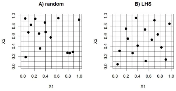
reste abordable dans le cas de modèles (semi-)analytiques à l’instar de celui utilisé pour la "pente infinie". Cependant, les estimations de l’aléa peuvent se baser sur des modèles numériques dont le temps de calcul n’est pas négligeable (plusieurs minutes voire heures). Par exemple, ce temps de calcul peut s’expliquer par l’obligation de traiter l’évaluation à grande échelle et donc d’utiliser des maillages avec un grand nombre de mailles/cellules (e.g., évaluation de la susceptibilité de glissement de terrain à l’échelle d’un bassin versant). Un autre exemple est un modèle numérique d’un glissement de terrain prenant en compte le couplage entre processus mécaniques et hydrauliques, dont la résolution numérique peut être ardue. Afin de surmonter ce problème, nous avons proposé de combiner VBSA avec la technique de méta-modélisation, qui consiste à capturer la relation mathématique entre les paramètres d’entrée et la variable de sortie du modèle numérique via une approximation mathématique construite avec un nombre restreint de simulations intensives (typiquement 50-100). 0 2 4 6 8 10 −10 −5 0 5 10 A) x y ● ● ● ● ● ● 0 2 4 6 8 10 −10 −5 0 5 10 B) x y ● ● ● ● ● ● ● ● ● ● True function Approximation

FIGURE2 – Approximation d’un modèle 1d (rouge) par un méta-modèle de type krigeage (en

noir) construit à partir des configurations indiquées par des points rouges : A) 6 simulations différentes ; B) 10 simulations différentes.

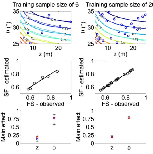
Plusieurs types de méta-modèles existent et nous nous sommes concentrés sur le krigeage numérique. Cette technique repose sur les outils d’interpolation spatiale de la géostatistique. Dans notre cas, les valeurs interpolées ne sont pas des coordonnées géographiques, mais sont

les paramètres d’entrée du modèle numérique. A titre illustratif, la figure2donne l’exemple

d’une fonction simple avec un paramètre d’entrée x : y = x(cos(x) + sin(x)) (en rouge) qui est

approximée (en noir) en utilisant soit 6 (figure2A)) ou 10 (figure2B)) différentes configurations

(valeurs) du paramètre x (points rouges). Le krigeage est associé à une tendance constante et

une fonction de corrélation de type Matérn sans effet pépite. La figure2montre que seulement

Cette stratégie a été appliquée au cas réel du glissement de terrain de La Frasse (Suisse) dont le modèle numérique a un temps de calcul de plusieurs jours, car le comportement rhéologique du matériau au niveau de la surface de glissement suit une loi complexe (loi Hujeux). A partir d’un nombre limité de simulations (ici une trentaine), nous avons pu approximer les déplacements horizontaux en surface en fonction des valeurs des propriétés du matériau constituant la surface de glissement. En vérifiant la qualité d’approximation par une méthode par validation croisée, nous avons remplacé le code numérique couteux en temps de calcul par le méta-modèle et avons ainsi pu dériver les effets principaux (indices de Sobol’ de 1er ordre) pour étudier la sensibilité sur les déplacements. Cependant, un prix à payer fut l’introduction d’une nouvelle source d’incertitude, i.e. celle liée au fait que l’on a remplacé le vrai modèle

par une approximation. La figure2A) illustre ce problème : la partie droite n’est pas bien

approximée à cause du manque d’information (aucune simulation réalisée dans cette partie). L’impact de cette erreur sur les résultats de VBSA a été discuté en associant un intervalle de confiance aux indices de sensibilité via un traitement du problème d’apprentissage du méta-modèle dans le cadre Bayésien. Bien qu’il faille souligner la complexité de mise en oeuvre ainsi que la sensibilité aux hypothèses (en particulier aux lois de probabilité a priori), cette stratégie "méta-modèle-VBSA-traitement Bayésien" nous a permis d’apporter des éléments de réponse à la question de l’influence des sources d’incertitudes paramétriques en un temps limité et raisonnable (quelques jours incluant les simulations et la construction du méta-modèle) et avec un nombre restreint de simulations (ici une trentaine).

0.2 Limitation n°2 : gérer des paramètres variant dans l’espace et le

temps

La seconde limitation est liée à la nature des paramètres dans le domaine des aléas géotech-niques : ce sont souvent des fonctions complexes du temps et/ou de l’espace et non pas simplement des variables scalaires. En d’autres termes, ces paramètres sont souvent repré-sentés par des vecteurs de grande dimension (typiquement 100-1000). Un exemple sont les

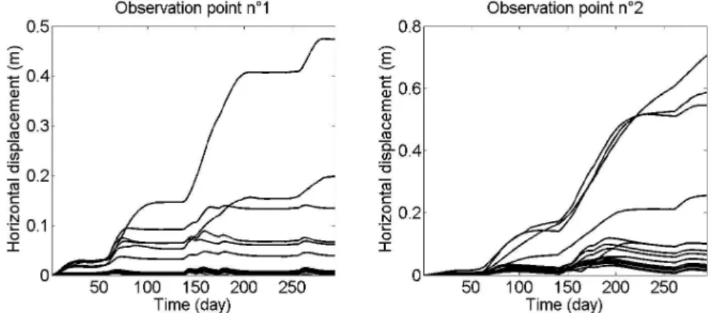
séries temporelles des déplacements horizontaux (Fig.3B) et C)) simulés à La Frasse lors de

la variation de la pression de pore en pied de glissement de terrain (Fig.3A)) : ces séries sont

obtenues à tous les noeuds du maillage et sont discrétisées sur 300 pas de temps. Un autre exemple est la carte hétérogène des conductivités hydrauliques d’un sol.

Une première démarche consisterait à évaluer un indice de sensibilité à chaque pas de temps en utilisant les techniques décrites ci-avant. Cependant, cette démarche serait difficilement réalisable avec des vecteurs de très grande dimension et ne permettrait pas de prendre en compte la corrélation qui peut exister (dans l’exemple des séries temporelles, une valeur à un temps donné a un lien avec celles d’avant et celles d’après). Dans un premier temps, nous nous sommes focalisés sur le cas des séries temporelles des déplacements horizontaux dans

FIGURE3 – Illustration des séries temporelles qui sont en entrée (pression de pore A)) et en sortie du modèle numérique simulant le glissement de La Frasse (glissements horizontaux en tête B) et en pied de glissement C)). La courbe rouge correspond à la moyenne temporelle.

le cas du glissement de La Frasse. Nous avons alors proposé une stratégie combinant : • des techniques de réduction de la dimension, en particulier l’analyse des composantes

principales ;

• un méta-modèle pour surmonter le coût calculatoire des indices de sensibilité. La première étape permet de résumer l’information temporelle en décomposant les séries temporelles en un nombre restreint de paramètres (<3), qui correspondent aux composantes principales. Une analyse plus "physique" de ces composantes principales est faite en les interprétant comme une perturbation de la moyenne temporelle (courbe rouge sur la figure

3B) et C)) : cela permet alors d’identifier les principaux modes de variation temporelles

pouvant être vus comme un enchaînement de phases de déstabilisation ou de stabilisation du glissement. Les indices de sensibilité calculés via le méta-modèle sont alors associés à chaque composante principale, i.e. à chaque mode de variation temporelle. Une telle démarche permet par exemple d’identifier les propriétés incertaines les plus importantes au regard de l’occurence d’une phase d’accélération lors du glissement sur une période donnée.

L’applicabilité de ce type de stratégie a aussi été discutée pour les paramètres d’entrée fonc-tionnels en se focalisant sur ceux spatialisés. Dans ce cas, la stratégie se trouve être limitée : 1. le nombre de composantes dans la décomposition reste important (plusieurs dizaines), i.e. assez grand pour rendre difficile la phase d’apprentissage (construction) du méta-modèle, qui est directement liée à ce nombre ; 2. le niveau auquel la décomposition peut être tronquée est décidé avant d’avoir pu lancer les simulations, i.e. avec peu de possibilité de savoir en amont si une partie de l’information laissée de côté pourrait avoir un impact sur la qualité d’approximation du méta-modèle ; 3. l’interprétation physique de chaque mode de variation peut être difficile. Sur cette base, des pistes de recherche ont été identifiées.

0.3 Limite n°3 : gérer le manque de connaissance

Enfin, une troisième limite est liée à l’hypothèse de base sur la représentation de l’incertitude. Par construction, VBSA repose sur les outils du cadre probabiliste avec l’hypothèse que la variance capture de façon satisfaisante toute l’incertitude sur la variable d’intérêt. Or, cette approche peut être limitée surtout dans le domaine des aléas géotechniques, pour lesquels les données / informations sont souvent imprécises, incomplètes voire vagues. Dans ce contexte de connaissance, l’utilisation systématique des probabilités peut être discutable. Une revue des principales critiques est faite et l’applicabilité d’un outil alternatif pour la représentation

de l’incertitude est étudiée, à savoir les ensembles flous. La figure4A) donne l’exemple d’un

ensemble flou (définissant formellement une distribution de possibilités), qui permet de représenter une information d’expert du type : "je suis sûr de trouver la vraie valeur du paramètre incertain dans l’intervalle [a ;d] (support), mais l’intervalle [b ;c] (coeur) a plus de vraisemblance." A partir de ces deux informations, un ensemble d’intervalles emboîtés associés à un degré de confiance (α-coupe) est construit. Son interprétation dans le domaine

des probabilités est donnée sur la figure4B). Une telle représentation correspond à l’ensemble

de distributions cumulées de probabilités dont les limites hautes et basses (Π et N) sont construites à partir des informations sur le coeur et le support.

FIGURE4 – A) Exemple d’un intervalle flou pour représenter l’imprécision d’un paramètre

incertain à partir de l’information d’expert sur le support et le coeur. B) Interprétation dans le domaine des probabilités via les 2 distributions cumulées, haute Π et basse N.

Un ensemble flou est un outil très flexible pour traiter plusieurs formes d’incertitudes épisté-miques :

• la représentation du caractère vague de l’information est abordée pour l’évaluation de la susceptibilité de présence de cavités à l’échelle régionale ;

• le raisonnement à partir de concepts qualitatifs vagues est traité dans le cas de l’impré-cision liée à l’inventaire des éléments à risque pour un scénario de risque sismique à l’échelle d’une ville ;

• l’imprécision sur la valeur numérique d’un paramètre (comme illustrée par la figure3) est abordée pour l’évaluation du coefficient d’amplification représentant les effets de site lithologique en risque sismique ;

• l’imprécision sur les valeurs des paramètres d’une courbe de décision probabiliste est abordée dans le domaine sismique.

Sur cette base, les principales procédures pour combiner représentation hybride des incerti-tudes (e.g., via probabilités et ensembles flous) et analyse de sensibilité sont étudiées. Une limitation majeure a été identifiée, à savoir le coût calculatoire : alors que la propagation dans le cadre purement probabiliste peut se baser sur des méthodes d’échantillonnage aléatoire exigeant basiquement de simuler différentes configurations des paramètres d’entrée, les nou-velles théorie de l’incertain exige souvent de manipuler des intervalles et donc de résoudre des problèmes d’optimisation. Une possible réponse à ce problème a été proposée en développant un outil graphique pour les analyses de stabilité. Une caractérisque intéressante est que cet outil n’est construit qu’à partir des simulations nécessaires à la propagation d’incertitude, donc sans coût calculatoire supplémentaire. Cet outil permet de placer sur le même niveau de comparaison, incertitude aléatoire et épistémique et donc d’identifier les contributions de chaque type d’incertitude à l’évaluation d’une probabilité de défaillance. Cette approche est appliquée à trois cas pour lesquels l’utilisation des probabilités est discutable pour représenter des paramètres imprécis : i. le cas d’un glissement de terrain dont les caractéristiques géomé-triques sont mal connues ; ii. le cas de la rupture d’un pilier dans une carrière abandonnée dont le taux d’extraction est difficilement évaluable à cause de la configuration particulière de la carrière ; iii. le cas de la rupture d’un pilier en calcaire présentant de fines couches argileuses dont les propriétés sont difficilement évaluables in situ. Notons que le cas iii. a exigé de développer une approche basée sur les méta-modèles, car l’évaluation de la stabilité du pilier exigeait un code numérique coûteux en temps de calcul.

La figure5donne l’exemple d’un résultat de l’outil graphique pour l’évaluation de stabilité

d’une falaise d’angle de frottement φ (supposée être un paramètre aléatoire représenté par une

distribution de probabilités) et de hauteur Htdu pied de falaise (supposée être un paramètre

imprécis représenté par une distribution de possibilités) : plus la courbe dévit de la diagonale, plus le paramètre a une grande influence : ici c’est l’angle φ. En pratique, ce résultat indique que les futures actions en matière de gestion des risques devraient reposées sur des mesures préventives et/ou de protection, car ce paramètre est associé à une variabilité naturelle : l’incertitude ne peut donc pas être réduite. De plus, la portion du graphique où la déviation est maximale indique la région des quantiles de l’angle φ et la région des α-coupes de la hauteur

Ht pour laquelle le paramètre est le plus influent : ici, cela correspond respectivement à la

région des quantiles inférieurs à 75% de l’angle φ et à celle proche du coeur de Ht. Ce simple

0.0 0.2 0.4 0.6 0.8 1.0 0.0 0.2 0.4 0.6 0.8 1.0 q CFP φ Ht

FIGURE5 – Analyse de sensibilité avec l’outil graphique pour le cas d’une falaise dont le

matériau a un angle de frottement aléatoire φ et de hauteur de pied de falaise Htimprécis.

pour la gestion des incertitudes selon leur nature (épistémique ou aléatoire).

0.4 En résumé...

L’apport de cette thèse est avant tout d’ordre méthodologique. En se basant sur des techniques avancées dans le domaine de l’analyse statistique (indices de Sobol’, techniques de réduction de dimension, ensembles flous, variables aléatoires flous, etc.), nous essayons d’apporter des réponses à des questions opérationnelles en matière de traitement des incertitudes dans l’évaluation des aléas géotechniques (glissement de terrain, séismes, cavités abandonnées, etc.), à savoir : quelle source d’incertitude doit être réduite en priorité ? Comment manipuler des codes de calcul avec un temps de calcul de plusieurs heures pour simuler de multiples scénarios (e.g., plusieurs centaines) ? Comment aborder la question des incertitudes lorsque les seules informations disponibles sont des opinions d’experts qualitatives et quelques obser-vations quantitatives ? Ce travail repose soit sur une combinaison de plusieurs techniques, ou sur une adaptation de certaines d’entre elles. Un effort tout particulier a été fait pour étudier l’applicabilité de chaque procédure à l’aune de données sur des cas réels.

Le présent document a été rédigé sur la base des travaux de recherche que j’ai effectués au BRGM (Service géologqiue national) depuis 2010. La thèse repose sur quatre articles (trois en tant qu’auteur principal et un en tant que co-auteur), à savoir :

• Nachbaur, A., Rohmer, J., (2011) Managing expert-information uncertainties for asses-sing collapse susceptibility of abandoned underground structures. Engineering Geology, 123(3), 166–178 ;

• Rohmer, J., Foerster, E., (2011) Global sensitivity analysis of large scale landslide numeri-cal models based on the Gaussian Process meta-modelling. Computers and Geosciences, 37(7), 917-927 ;

• Rohmer, J., (2013) Dynamic sensitivity analysis of long-running landslide models through basis set expansion and meta-modelling. Natural Hazards, accepted, doi :10.1007/s11069-012-0536-3 ;

• Rohmer, J., Baudrit, C., (2011) The use of the possibility theory to investigate the episte-mic uncertainties within scenario-based earthquake risk assessments. Natural Hazards, 56(3), 613-632.

En plus de ces travaux, un étude originale a été effectuée en collaboration avec mon directeur de thèse, Thierry Verdel, et a été intégrée dans le présent manuscrit. Ce travail a également été publié récemment.

• Rohmer, J., Verdel, T. (2014) Joint exploration of regional importance of possibilistic and probabilistic uncertainty in stability analysis. Computers and Geotechnics, 61, 308–315. Lors de l’écriture, un effort tout particulier a été fait afin que le manuscrit ne soit pas un « simple » résumé de ces travaux, mais que le document ait une cohérence d’ensemble et forme un « tout ». Dans cette optique, plusieurs parties ont été réécrites par rapport aux articles originaux. Par ailleurs, des détails techniques ont été ajoutés dans un souci de clarté de l’énoncé.

The present thesis summarises the research I have undertaken at BRGM (French geological survey) since 2010 on uncertainty treatment in various natural hazards: landslide, earthquake and abandonned underground structures. The thesis is strongly based on four peer-reviewed publications (three as first author and one as co-author):

• Nachbaur, A., Rohmer, J., (2011) Managing expert-information uncertainties for assess-ing collapse susceptibility of abandoned underground structures. Engineerassess-ing Geology, 123(3), 166–178;

• Rohmer, J., (2013) Dynamic sensitivity analysis of long-running landslide models through basis set expansion and meta-modelling. Natural Hazards, accepted, doi:10.1007/s11069-012-0536-3;

• Rohmer, J., Foerster, E., (2011) Global sensitivity analysis of large scale landslide numeri-cal models based on the Gaussian Process meta-modelling. Computers and Geosciences, 37(7), 917-927.

• Rohmer, J., Baudrit, C., (2011) The use of the possibility theory to investigate the epis-temic uncertainties within scenario-based earthquake risk assessments. Natural Haz-ards, 56(3), 613-632.

In addition to these studies, an original research work has been conducted with my thesis advisor, Thierry Verdel, and added to the thesis. This was publised recently:

• Rohmer, J., Verdel, T. (2014) Joint exploration of regional importance of possibilistic and probabilistic uncertainty in stability analysis. Computers and Geotechnics, 61, 308–315 A special attention has been paid to go beyond a “simple” summary of the main contents of the different research papers: some parts were re-written for sake of coherency of the whole document and additional technical details were added for sake of clarity.

Acknowledgements i

Technical Summary iii

Résumé étendu vii

0.1 Limitation n°1 : gérer le temps de calcul . . . viii

0.2 Limitation n°2 : gérer des paramètres variant dans l’espace et le temps . . . x

0.3 Limite n°3 : gérer le manque de connaissance . . . xii

0.4 En résumé... . . xiv

Foreword xvii

List of figures xxiii

List of tables xxvii

1 Introduction 1

1.1 Hazard, Risk, uncertainty and decision-making . . . 1

1.2 Aleatory and Epistemic uncertainty . . . 3

1.3 Epistemic uncertainty of type "parameter" . . . 5

1.4 A real-case example. . . 6

1.5 Objectives and structure of the manuscript. . . 7

2 A probabilistic tool: variance-based global sensitivity analysis 11

2.1 Global sensivity analysis . . . 11

2.2 Variance-based global sensivity analysis . . . 13

2.3 Application to slope stability analysis . . . 15

2.3.1 Local sensitivity analysis. . . 16

2.3.2 Global sensitivity analysis . . . 18

3 Handling long-running simulators 23

3.1 A motivating real case: the numerical model of the La Frasse landslide . . . 23

3.1.1 Description of the model . . . 23

3.1.2 Objective of the sensitivity analysis . . . 24

3.2 A meta-model-based strategy . . . 25

3.2.1 Principles . . . 25

3.2.2 Step 1: setting the training data. . . 26

3.2.3 Step 2: construction of the meta-model. . . 27

3.2.4 Step 3: validation of the meta-model . . . 28

3.3 A flexible meta-model: the kriging model . . . 29

3.4 An additional source of uncertainty . . . 31

3.5 Application to an analytical case . . . 34

3.6 Application to the La Frasse case . . . 36

3.7 Concluding remarks of Chapter 3. . . 43

4 Handling functional variables 45

4.1 Problem definition for functional outputs . . . 45

4.2 Reducing the dimension . . . 47

4.2.1 Principles . . . 47

4.2.2 Principal Component Analysis . . . 48

4.2.3 Interpreting the basis set expansion . . . 49

4.3 Strategy description . . . 51

4.3.1 Step 1: selecting the training samples . . . 52

4.3.2 Step 2: reducing the model output dimensionality . . . 52

4.3.3 Step 3: constructing the meta-model . . . 52

4.3.4 Step 4: validating the meta-model . . . 54

4.4 Application to the La Frasse case . . . 55

4.4.1 Construction of the meta-model . . . 55

4.4.2 Computation and analysis of the main effects . . . 56

4.5 Towards dealing with functional inputs . . . 58

4.5.1 Strategy description . . . 58

4.5.2 Case study . . . 59

4.5.3 Discussion . . . 60

4.6 Concluding remarks of Chapter 4. . . 62

5 A more flexible tool to represent epistemic uncertainties 67

5.1 On the limitations of the systematic use of probabilities . . . 67

5.2.1 A motivating real-case: hazard related to abandoned underground struc-tures . . . 71

5.2.2 Membership function . . . 72

5.2.3 Application . . . 73

5.3 Reasoning with vagueness . . . 75

5.3.1 A motivating real-case: the inventory of assets at risk . . . 75

5.3.2 Application of Fuzzy Logic . . . 76

5.4 Handling imprecision . . . 79

5.4.1 Possibility theory . . . 79

5.4.2 A practical definition . . . 80

5.4.3 Illustrative real-case application . . . 81

5.5 Handling probabilistic laws with imprecise parameters . . . 82

5.5.1 A motivating example: the Risk-UE (level 1) model . . . 82

5.5.2 Problem definition . . . 83

5.5.3 Use for an informed decision . . . 84

5.6 Concluding remarks of Chapter 5. . . 86

6 Sensitivity analysis adapted to a mixture of epistemic and aleatory uncertainty 89

6.1 State of the art of sensitivity analysis accounting for hybrid uncertainty repre-sentations . . . 89

6.2 A graphical-based approach. . . 93

6.2.1 Motivation . . . 93

6.2.2 Joint propagation of randomness and imprecision . . . 94

6.2.3 Contribution to probability of failure sample plot . . . 97

6.2.4 Adaptation to possibilistic information . . . 98

6.3 Case studies . . . 99

6.3.1 Simple example . . . 99

6.3.2 Case study n°1: stability analysis of steep slopes . . . 100

6.3.3 Case study n°2: stability analysis in post-mining . . . 103

6.3.4 Case study n°3: numerical simulation for stability analysis in post-mining106

6.4 Concluding remarks for Chapter 6 . . . 111

7 Conclusions 115

7.1 Achieved results . . . 115

7.2 Open questions and Future developments . . . 118

7.2.1 Model uncertainty . . . 118

A Functional decomposition of the variance: the Sobol´ indices 123

B Universal kriging equations 127

C Key ingredients of a bayesian treatment of kriging-based meta-modelling 131

C.1 Principles of Bayesian Model Averaging . . . 131

C.2 Monte-Carlo-based procedures. . . 132

C.3 Bayesian kriging. . . 133

C.4 Deriving a full posterior distribution for the sensitivity indices . . . 135

D Brief introduction to the main uncertainty theories 137

D.1 Probability . . . 137

D.2 Imprecise probability. . . 138

D.3 Evidence theory . . . 138

D.4 Probability bound analysis . . . 139

D.5 Possibility theory . . . 140

E Fuzzy Random Variable 141

1 Exemple d’un résultat dérivant dune analyse globale de sensibilité à partir des indices de Sobol’ de 1er ordre et indices totaux. . . viii

2 Approximation d’un modèle 1d par un méta-modèle de type krigeage construit à partir des configurations indiquées par des points rouges. . . ix

3 Illustration des séries temporelles qui sont en entrée et en sortie du modèle numérique simulant le glissement de La Frasse. . . xi

4 Exemple d’un intervalle flou pour représenter l’imprécision d’un paramètre incertain à partir de l’information d’expert sur le support et le coeur. . . xii

5 Analyse de sensibilité avec l’outil graphique pour le cas d’une falaise dont le matériau a un angle de frottement aléatoire φ et de hauteur de pied de falaise Ht.xiv

1.1 Example of a uncertainty classification. . . 6

1.2 La Frasse landslide topview and model. . . 7

1.3 Generic framework for uncertainty treatment . . . 9

2.1 Infinite slope model. . . 16

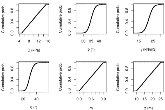
2.2 Uncertainty assumptions for infinite slope model. . . 17

2.3 Application of OAT on the infinite slope model considering different cases of shifting parameters and reference values. . . 18

2.4 VBSA for infinite slope model. . . 19

2.5 Scatterplots for two parameters of the infinite slope model. . . 20

3.1 Random generation of variables versus LHS (maximin criterion) . . . 27

3.2 Illustration of kriging meta-modelling technique with the infinite slope model. 35

3.3 Horizontal displacements at two observation points of the La Frasse model. . . 37

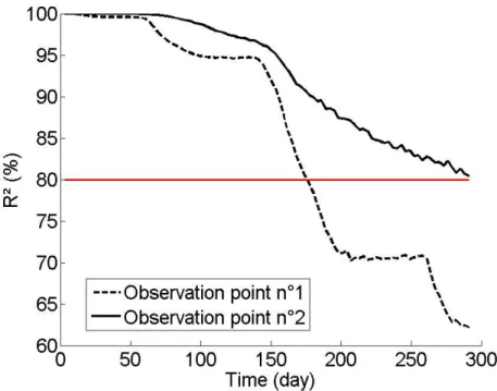
3.4 Cross-validation of the meta-model for the La Frasse case.. . . 38

3.5 Traceplots for three parameters of the kriging meta-model of the La Frasse model. 39

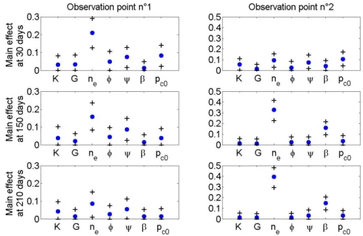
3.6 Temporal evolution of the main effects of the 1st and 2nd most important pa-rameters in the La Frasse case. . . 40

4.1 Time series in the La Frasse landslide model.. . . 46

4.2 PCA applied to the La Frasse landslide model (upper part). . . 50

4.3 Comparison between observed and PCA-reconstructed time series. . . 51

4.4 PCA applied to the La Frasse landslide model (lower part).. . . 52

4.5 Validation of the functional meta-model of La Frasse. . . 56

4.6 VBSA applied to the La Frasse case using PCA. . . 57

4.7 Spatially varying input: example and approximation through PCA.. . . 60

4.8 Differences between the original and the approximated maps. . . 61

4.9 Choice of the optimal number of PCs in the decomposition of the spatially-varying input. . . 62

4.10 Maps of the PCs related to the expansion of a spatially-varying input. . . 63

5.1 Illustration of the limitations of using uniform probability distributions in situa-tions of lack of knowledge.. . . 69

5.2 Graphical representation of the set A under the classical Boolean theory and under the fuzzy set theory.. . . 73

5.3 Construction of the membership function associated to the criterion for cavity susceptibility assessment. . . 74

5.4 Situation of the French city of Lourdes - Assets at risks and geotechnical zonation. 76

5.5 Methodology for inventory imprecision assessment adapted from the approxi-mate reasoning of [Zadeh, 1975]. . . 78

5.6 Illustration of a possibility distribution associated with an imprecise parameter (A) and definition of the measure of possibility and necessity (B).. . . 80

5.7 Illustration of the family of probabilistic damage curves associated to the α-cuts of the imprecise parameter rD. . . 84

5.8 Synthesis in a pair of probabilistic indicators of all the possible alternatives for the probabilistic damage curves associated with the α-cuts of the imprecise parameter rD. . . 85

5.9 Mapping of the lower and upper probabilistic indicator of the event: “exceeding damage grade D4”. . . 86

6.1 Example of pinching transformation of the fuzzy set assigned to the vulnerability index Vi of the M4 class of vulnerability. . . 91

6.2 Epistemic indicator as function of the filter width Vf applied to the fuzzy set of

6.3 Main steps of the joint propagation of a random variable represented by a cu-mulative probability distribution and an imprecise variable represented by a cumulative possibility distribution using the independence Random Set proce-dure of [Baudrit et al., 2007b].. . . 95

6.4 CFP curves associated with the random variable ǫ and the imprecise variable X considering different cases of “randomness strength r ”. . . . 100

6.5 Schematic description of the failure geometry applied in [Collins and Sitar, 2010] to assess stability of steep slopes in cemented sands. . . 101

6.6 Plausibility and Belief functions resulting from the joint propagation of variabil-ity and imprecision in the slope stabilvariabil-ity analysis. . . 102

6.7 CFP curves associated with the random and imprecise variables of the slope stability analysis. . . 103

6.8 Schematic representation of the underground quarry of Beauregard (adapted from [Piedra-Morales, 1991]). . . 104

6.9 CFP curves associated with the random and imprecise variables of the mine pillar stability analysis. . . 105

6.10 A) Model geometry and boundary conditions for evaluating the stress evolution at mid height of pillar during loading; B) Map of plastic shear strain at the end of the loading; C) Typical stress evolution during loading.. . . 107

6.11 Leave-One-Out Cross-Validation procedure applied to both kriging-type meta-models for the lower and upper bounds of the average stress. . . 110

6.12 Upper and Lower probability distribution bounding the true probability assigned to the average stress at the end of loading. . . 111

6.13 CFP derived from the joint propagation of imprecision and randomness for the pillar case. . . 112

2.1 Assumptions for uncertainty representation of the infinite slope model. . . 16

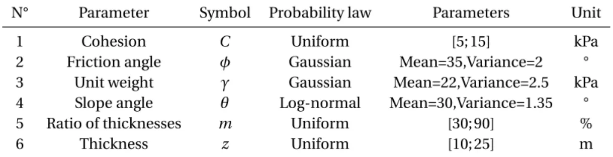
3.1 Range of values for the slip surface properties of the La Frasse landslide. . . 25

3.2 Main steps of the meta-modelling strategy for global sensitivity analysis using computationally intensive numerical models. . . 26

3.3 Comparison between the “true” and the estimates of the main effects for the infinite slope analytical model. . . 36

4.1 Main steps of the meta-modelling strategy for dynamic sensitivity analysis using

PCA.. . . 53

5.1 Numerical choices for imprecision assessment considering the inventory of assets at risk at Lourdes. . . 77

5.2 Logical rules for imprecision assessment considering the inventory of assets at risk at Lourdes. . . 77

5.3 Imprecision assessment in the district n°18. . . 79

6.1 Description of the main steps and methods of the joint exploration procedure of possibilistic and probabilistic uncertainty.. . . 98

6.2 Assumptions on the uncertainty representation for the properties of the rock materials composing the mine pillar. . . 108

The present PhD thesis focuses on the treatment of uncertainty in the assessments of

“geo-hazards”. These types of hazard (see Sect. 1.1for a definition) are related to geological or

geotechnical phenomena like earthquake, landslide, sinkhole, etc. Such hazards are generally categorized as natural hazards, but their origin can be of anthropogenic nature as well, an

ex-ample being mining subsidences [Deck and Verdel, 2012]. When it comes to making informed

choices for the management of geo-hazards (through risk reduction measures, land use plan-ning or mitigation strategies, etc.), the issue of uncertainty is of primary importance (see [Hill et al., 2013] and references therein). Uncertainties should be recognized (i.e. identified) and their implications should be transparently assessed (i.e. propagated), honestly reported

and effectively communicated as underlined by [Hill et al., 2013]. In Sect.1.1, the notion of

uncertainty is clarified and defined through its relationship with risk and decision-making. In

Sect.1.2, two facets of uncertainty are outlined, namely “aleatory” and “epistemic uncertainty”.

The latter facet is at the core of the present work, and more specifically the lack of knowledge,

designated as “parameter uncertainty” in the following (Sect. 1.3). This type of epistemic

uncertainty is illustrated with the real-case of the La Frasse landslide (Sect.1.4). On this basis,

the major research questions are raised, which constitute the lines of research of the present

work (Sect.1.5).

1.1 Hazard, Risk, uncertainty and decision-making

Natural risks can be understood as the combination of hazard and of vulnerability. A hazard can be defined as “a potentially damaging physical event, phenomenon or human activity that may cause the loss of life or injury, property damage, social and economic disruption or

environmental degradation” [UN/ISDR, 2004]. Vulnerability can be defined as “the conditions

increase the susceptibility of a community to the impact of hazards” [UN/ISDR, 2004]. However, it should be underlined that the definition of risk is not unique and the glossary on

components of risk provided by the United Nations University [Thywissen, 2006] is composed

of more than 20 definitions. In all those definitions, the situation of risk is always understood relative to the situation of uncertainty using terms that can, in a broad sense, be related to the concept of uncertainty (expectation, probability, possibility, unknowns, etc.). Besides, it is interesting to note that the ISO standard ISO 31000:2009 on risk management defines risk as the “effect of uncertainty on objectives”.

[Knight, 1921] provided an original vision on the relationship between risk and uncertainty by formally distinguishing both concepts as follows: in a situation of risk, the probability of each possible outcome can be identified, whereas in a situation of uncertainty, the outcome can

be identified, but not the corresponding probabilities ([Knight, 1921], quoted by [Bieri, 2006]).

Traditionally, rational decision-making under uncertainty is based on probabilities using the

Independence Axiom introduced by [Von Neumann and Morgenstern, 1944] and extended

by [Savage, 1954]. Under very general conditions, the independence axiom implies that the individual objective is linear in probabilities. This leads to the subjective expected utility theory under which decision support should only be guided by the values of probabilities. Yet, within this formalism, the nature and quantity of information that have led to the estimate

of the probability values does not influence the decision. As underlined by [Paté-Cornell, 2002],

according to this theory, the rational decision maker is indifferent to two sources of information that result in the same probabilistic distribution of outcomes, i.e. regardless of whether they result from experiments based on flipping a coin, or following a “rain tomorrow” approach

(let say, based on the “weatherman’s opinion”). [Keynes, 1921] originally provided a view on

this issue by distinguishing between probability and “weight of evidence”, so that probability represents the balance of evidence in favour of a particular option, whereas the weight of evidence represents the quantity of evidence supporting the balance. According to this view, people should be more willing to act if the probability of an outcome is supported by a larger

weight of evidence, i.e. the situation is less “ambiguous”. The work of [Ellsberg, 1961] has

provided experimental evidence that people do not behave in the same way in the face of two uncertain environments with the same probabilities, but with different weights of evidence (i.e., different degrees of ambiguity). In their well-known classic experiment, subjects prefer to take a chance on winning a prize with draws from an urn with a specified mixture of balls as opposed to taking a chance with a subjective probability that is equivalent, but ambiguous. Since these original works, extensive work have been carried out to better understand the complex relationship between uncertainty, ambiguity and information and how this affects

decision-making (see, e.g., [Cabantous et al., 2011] and references therein). Consequently, recent studies on risk analysis have outlined that the relationship between risk and uncertainty

through probabilities may be too restrictive. For instance, [Aven and Renn, 2009] define risk in

a broader sense as the “uncertainty about and sensitivity of the consequences (and outcomes) of an activity with respect to something that humans value”.

1.2 Aleatory and Epistemic uncertainty

Giving a single “fit-to-all” definition for uncertainty remains difficult, because uncertainty can be interpreted differently depending on the discipline and context where it is applied, as

outlined for instance by [Ascough(II) et al., 2008] in environmental and ecological studies.

Therefore, several authors [van Asselt and Rotmans, 2002, Rogers, 2003, Walker et al., 2003,

Baecher and Christian, 2005,Cauvin et al., 2008], among others, adopt a less ambitious (but more practical) approach by defining uncertainty through classification. Such an approach presents the appealing feature of enabling the risk practitioners to differentiate between uncertainties and to communicate about them in a more constructive manner.

Though differing from one classification to another, they have all in common to distin-guish two major facets of uncertainty, namely “aleatory uncertainty” and “epistemic un-certainty”. In the domain of natural hazards, the benefits of distinguishing both facets have

been outlined for geo-hazards by [Deck and Verdel, 2012], and more specifically for seismic

risk by [Abrahamson, 2000], for rockfall risk by [Straub and Schubert, 2008], for volcano risk

by [Marzocchi et al., 2004].

• The first facet corresponds to aleatory uncertainty/variability (also referred to as ran-domness). The physical environment or engineered system under study can behave in different ways or is valued differently spatially or/and temporally. The aleatory variabil-ity is associated with the impossibilvariabil-ity of predicting deterministically the evolution of a system due to its intrinsic complexity. Hence, this source of uncertainty represents the “real” variability and it is inherent to the physical environment or engineered system

under study, i.e., it is an attribute/property;

• The second facet corresponds to epistemic uncertainty. This type is also referred to as “knowledge-based”, as the latin term episteme means knowledge. Contrary to the first type, epistemic uncertainty is not intrinsic to the system under study and can be qualified as being “artificial”, because it stems from the incomplete/imprecise nature of available information, i.e., the limited knowledge of the physical environment or engineered system under study. Epistemic uncertainty encompasses a large variety of

It is worth stating that both sources of uncertainty can be inter-connected so that the study of a stochastic system is by its nature pervaded by randomness, but the resources to measure and obtain empirical information on such a stochastic system can be limited, i.e., uncertainty can exhibit both variability and a lack of knowledge (epistemic uncertainty). Conversely, this aspect should not exclude the situation where knowledge with regard to deterministic

processes can also be incomplete [van Asselt and Rotmans, 2002], e.g., a wellbore has been

drilled, but its depth has not been reported so that it remains imprecisely known.

It should be recalled that the objective here is not to reopen the widely discussed debate on the

relevance of the separation of uncertainty sources (see e.g., [Kiureghian and Ditlevsen, 2009]).

Here, the scope is narrower and it is merely underlined that the efforts to separate both sources, though appearing as a "pure modelling choice", should be seen from a risk management

perspective as discussed by [Dubois, 2010]:

• Aleatory uncertainty, being a property of the system under study, cannot be reduced. Therefore, concrete actions can be taken to circumvent the potentially dangerous effects of such variability. A good illustration is the reinforcement of protective infrastructures such as the height of dykes to counter in a preventive fashion the temporal variations in the frequency and magnitude of storm surges. Another option can be based on the application of an additional "safety margin" for the design of the engineered structure; • Epistemic uncertainty, being due to the capability of the analyst (measurement

ca-pability, modeling caca-pability, etc.), can be reduced by, e.g., increasing the number of tests, improving the measurement methods or evaluating calculation procedure with model tests. In this sense, this type of uncertainty is referred to as "knowledge-based" [Kiureghian and Ditlevsen, 2009]. Given the large number of uncertainty sources, the challenge is then to set priorities, under budget/time constraints, on the basis of the identification of the most influential/important sources of uncertainty: this is at the core of the present PhD thesis.

From this viewpoint, it should be kept in mind that even in situations where a lot of infor-mation is available, uncertainty can still prevail, either because the system under study is by essence random (although epistemic uncertainty may have vanished through the increase of knowledge) or because new knowledge has illuminated some “not-yet-envisaged” com-plex processes, of which our understanding is still poor. This can be illustrated with the

earthquake on January 26th 2011 at Christchurch (New Zealand): an extreme shaking of

2.2 g was recorded whereas the magnitude is moderate of Mw=6.2 [Holden, 2011]. Hence,

the treatment of uncertainty is not only a matter of knowledge-gathering, but “the

[van Asselt and Rotmans, 2002]). Addressing uncertainty should therefore guide actions for risk management by identifying and ranking issues worthy to be tackled within the risk assess-ment procedure, which may concretely consist of collecting new data, but may also involve rethinking the assessment procedure, e.g., by comparing different points of views / experts’ judgments.

1.3 Epistemic uncertainty of type "parameter"

Epistemic uncertainty encompasses too many aspects to be practically used as a unique

concept, so that for the purposes of a risk analysis, [Cauvin et al., 2008] have suggested

distin-guishing between four classes of uncertainty (Fig.1.1adapted from [Deck and Verdel, 2012]).

• Resources uncertainty deals with knowledge about both the general scientific context of the study and its local particularities. More specifically, it concerns the existence of information about the processes being investigated and the objects being studied; • Expertise uncertainty is related to all the choices, actions or decisions that can be made

by the expert to carry out the risk study. It mainly relies on his/her particular experience as an individual, on his/her subjectivity and on the way he/she represents and interprets the information he/she has gathered;

• Model uncertainty is basically induced by the use of tools to represent reality and is related to the issue of model representativeness and reliability. This type of uncertainty is also named structural uncertainty defined as the failure of the model to represent the

system even if the correct parameters are known [Hill et al., 2013];

• Data uncertainty represents both the natural variability existing in the data, the lack of knowledge about their exact values and the difficulty of clearly evaluating them. The incomplete knowledge pervading the parameters of the models supporting geo-hazard assessment is at the core of the present work: this corresponds to the fourth category “Data

uncertainty” of [Cauvin et al., 2008]. As recently described by [Hill et al., 2013], this type of

epistemic uncertainty both encompasses parametric uncertainty (incomplete knowledge of the correct setting of the model’s parameters) and input uncertainty (incomplete knowledge of true value of the initial state and the loading). For sake of simplicity, this type of epistemic uncertainty is designated with the generic term “parameter uncertainty” in the present work. The term “parameter” is indifferently used to refer to the system’s initial state (e.g., initial stress state at depth), to the loading/forcing acting on the system (e.g., changes of groundwater table) and to the system’s characteristics (e.g. soil formation’s property).

Figure 1.1: Uncertainty classification in geo-hazard assessments as proposed by [Cauvin et al., 2008]. The “lack of knowledge” of the category “Data uncertainty” is at the core of the present work. It is referred to as “parameter uncertainty” in the present work.

1.4 A real-case example

To further clarify the concept of parameter uncertainty, let us consider the landslide of

"La Frasse" (Swiss), which has been studied by Laloui and co-authors [Laloui et al., 2004,

Tacher et al., 2005]. This landslide with active mass of ≈ 73 million m3, is located in the Pre-alps of the Canton of Vaud in Switzerland (at ≈ 20 km east from Lake Geneva) and has experienced several crises in the past, during which a maximum observed velocity of 1 m/week could be observed in the lower part of the landslide. An overview of the landslide is provided in

Fig.1.2A). The evolution of the groundwater table is considered to be at the origin of the sliding

and the instabilities were mainly observed during the 1994 crisis (over a period of nearly 300 days). Therefore, in order to assess the effect of the hydraulic regime on the geomechanical behaviour of the landslide, finite-element simulations considering a 2D cross-section through

the centre of the landslide were performed by [Laloui et al., 2004] using the finite element

program GEFDYN by [Aubry et al., 1986]. The model is composed of 1,694 nodes, 1,530

quad-rangular elements, and six soil layers derived from the geotechnical investigations. Figure

1.2B) gives an overview of the model, as well as the boundary conditions used for analysis.

Instabilities observed in 1994 were triggered by pore pressure changes occurring at the base of

the slide (see [Laloui et al., 2004] for further details).

The numerical model used for predicting the hydro-mechanical behaviour of the landslide involves a large variety of assumptions. The model involves model uncertainties related to:

• the system’s geometry: use of a two-dimensional cross section, spatial location of the slip surface, definition of six soil formations;

Figure 1.2: A) Topview of the La Frasse landslide in Switzerland. B) Overview of the two-dimensional finite-element model used for assessing the hydro-mechanical behaviour of the

La Frasse landslide (adapted from [Laloui et al., 2004]).

• the soil formations’ behaviour: spatially homogeneous properties, choice in the

consti-tutive law (Hujeux for the slip surface’s material [Hujeux, 1985] and Mohr Coulomb for

the others);

The model involves parameter uncertainties related to:

• the loading/forcing conditions of the system: the temporal evolution of the water level, location of the flow changes, nature of the boundary conditions (e.g., nil normal displacements and nil flow at the bottom);

• the properties’ values related to: the density, the initial stress state, the elastic behaviour (Young’s modulus, Poisson’s ratio), the plastic behaviour (internal friction angle, cohe-sion, dilatancy angle) and the flow behaviour (porosity, horizontal and vertical intrinsic permeability) of the six soil formations.

This real-case provides an example of an advanced numerical model used to support geo-hazard assessment. This shows that such models can involve a large number of sources of uncertainty. Considering only the input parameters, the La Frasse landslide model involves more than 50 parameters, i.e. more than 50 sources of uncertainty (not to mention the model uncertainties). A challenge for an efficient uncertainty treatment is then to reduce the number of uncertain parameters.

1.5 Objectives and structure of the manuscript

In the light of the afore-described real-case, the following question can be raised: among all the sources of parameter uncertainty, which of them have the greatest influence on the uncertainty associated to the results of the geo-hazard assessment? Which sources of uncer-tainty are the most important and should be taken into account in priority in the analysis?

How to rank the uncertain parameter in terms of importance? Conversely, which sources of uncertainty can be treated as insignificant and thus can be neglected in the analysis, i.e. how to simplify the model? Finally, on what parameters should the characterization effort be put in priority (additional lab tests, in site experiments, numerical simulations)? How to optimize the allocation of the resources for hazard assessment? Thus, the central research question is the importance ranking of parameter uncertainties (epistemic).

Addressing this question is of great interest in situations where the resources (time and budget) for hazard and risk assessments are generally limited. An example is the development of Risks

Prevention Plans, which are powerful operational and statutory tools [MATE, 1999], but their

practical implementation can be tedious as they impose to work “in the state of knowledge” and “according to expert opinion”, i.e. with no other resources that those available at the time

of the study, which, in practice, are generally limited as outlined by [Cauvin et al., 2008].

From a methodological perspective, this question falls into the goal for quantitative

uncer-tainty assessment termed as “Understand” [de Rocquigny et al., 2008]: “To understand the

influence or rank importance of uncertainties, thereby guiding any additional measurement, modelling or research efforts with the aim of reducing epistemic uncertainties”. This question is then related to the step of sensitivity analysis of the generic framework for uncertainty

treatment (Fig.1.3). The description of this generic framework is mainly based on the recent

best practices for uncertainty assessment ([de Rocquigny et al., 2008] in collaboration with

the European Safety Reliability Data Association). While sensitivity analysis (step 2’) focuses on the study of “how uncertainty in the output of a model (numerical or otherwise) can be

apportioned to different sources of uncertainty in the model input” [Saltelli et al., 2008], the

related practice of “uncertainty analysis” (step 2) focuses on the quantification of uncertainty in the model output. Step 2 and 2’ are usually run in tandem.

Several techniques exist in the literature to address the question of sensitivity analysis. Chapter

2first provides a brief overview of the main techniques for sensitivity analysis, and then,

focuses on the most commonly-used and most advanced tools for conducting sensitivity analysis in a global manner (Global Sensitivity Analysis GSA), namely techniques relying on

the decomposition of the variance in a probabilistic setting VBSA [Saltelli et al., 2008]. Using

a simple analytical model for landslide hazard assessment, this first chapter highlights how VBSA can be useful to answer the question related to importance ranking. On the other hand, this first chapter also highlights and discusses the main constraints for its practical implementation in the context of geo-hazard assessments, namely: