[ Journal of Legal Studies, vol. 45 (June 2016)]
© 2016 by The University of Chicago. All rights reserved. 0047-2530/2016/4502-0011$10.00
Black Sheep or Scapegoats? Implementable
Monitoring Policies under Unobservable
Levels of Misbehavior
Berno Buechel and Gerd Muehlheusser
ABSTRACT
An authority delegates a monitoring task to an agent. Thereby, it can observe the number of detected offenders but not the monitoring intensity chosen by the agent or the resulting level of misbehavior. We provide a necessary and sufficient condition for the implementability of monitoring policies. When several monitoring intensities lead to an observationally identical outcome, only the minimum of these is implementable, which can lead to underenforcement. A comparative-statics analysis reveals that increasing the punishment can undermine deterrence, since the maximal implementable monitoring intensity decreases. When the agent is strongly intrinsically motivated to curb crime, our results are mirrored, and only high monitoring inten-sities are implementable. Then, higher monetary rewards for detections lead to a lower moni-toring intensity and to a higher level of misbehavior.
1. INTRODUCTION
In many contexts of delegated monitoring, looking only at detection sta-tistics need not be informative about the quality of monitoring. For ex-ample, suppose a division head of a large company reports to corporate headquarters a low number of violations against some corporate code of conduct for his division (for example, compliance with certain ethical
berno buechel is a Postdoctoral Fellow at the Institute of Economics, University of St. Gallen, and at the Liechtenstein Institute. gerd muehlheusser is Professor of Economics at the University of Hamburg. We are grateful to William H. J. Hubbard and an anony-mous referee whose comments were very helpful in improving the paper. We also thank Eberhard Feess, Christos Litsios, Grischa Perino, Nicolas Sahuguet, Jan Schmitz, Urs Sch-weizer, Avi Tabbach, and Niklas Wallmeier as well as participants of the American Law and Economics Association meetings in 2014 (Chicago) and 2015 (New York) and semi-nars audiences at the University of Adelaide, the University of Bonn, Tel Aviv University, the University of Paderborn, and Paris West University Nanterre for their comments and suggestions.
332/ T H E J O U R N A L O F L E G A L S T U D I E S / V O L U M E 4 5 ( 2 ) / J U N E 2 0 1 6
or safety standards). Then, it is not obvious what this information re-veals about the true level of misbehavior in the division. A low number of detections could result from a strict monitoring policy that leads to few offenders, most of which are detected (black sheep). Instead, the monitor-ing policy could be lax, which leads to a large number of offenders, out of which only a few (scapegoats) are discovered. As a further example, in sports competitions it is hard for outsiders to judge what a given num-ber of detected dopers reveals about the seriousness and intensity of an-tidoping measures by the respective agencies and the virulence of doping among athletes. Further examples include offenses such as tax evasion, parking violations, prostitution, trafficking, and drug dealing, in which the number of detected offenders might not be very informative about the prevalence of an illegal activity.
The common feature of these examples is that an authority delegates the task of monitoring a population of individuals to an agent. Thereby, it is an outsider in the sense that it can neither observe the monitoring intensity chosen by the agent nor the resulting level of misbehavior.1 In contrast, the potential offenders have a good assessment of the proba-bility of being detected, which is a standard assumption in the economic literature on enforcement (see, for example, Polinsky and Shavell 2007).2 In this paper, we develop a simple model that captures the interaction among the authority, the monitoring agent, and potential offenders and that builds on the previous literature on private law enforcement with a monopolistic enforcer (see, for example, Becker and Stigler 1974; Landes and Posner 1975; Polinsky 1980; Besanko and Spulber 1989; Garoupa and Klerman 2002; Coşgel, Etkes, and Miceli 2011).
Some key features of our model can be foreshadowed with the fol-lowing simple example. The enforcement effort of the monitoring agent (the inspector) translates into p, the probability that an offense is detected and punished. The number of offenses committed is decreasing in the ex-pected punishment and, hence, decreasing in p for a given fine (T). For
1. The feature that several monitoring intensities lead to the same number of detec-tions also applies to many other settings such as education or loan audits. However, as discussed in Section 8, it is less clear in these contexts that the authority can be considered an outsider that has to rely on the number of reported detections only.
2. A similar informational structure is also considered in the model of Arlen (1994) in the context of corporate criminal liability. Moreover, as for the case of street prostitution, regular market participants might (correctly) perceive the actual threat of being arrested by the police (let alone convicted) to be much smaller than might be presumed by outsid-ers (see, for example, Levitt and Venkatesh 2007).
334/ T H E J O U R N A L O F L E G A L S T U D I E S / V O L U M E 4 5 ( 2 ) / J U N E 2 0 1 6
instance, Figure 1 depicts the number of offenses as a linear function F(p,
T) = 1 - pT for fine levels T = 1 and T = 2.3 Figure 1 also depicts the number of detections pF(p, T) for each case (dashed curves).
The example is helpful in illustrating the main contributions of our paper compared with the existing strands of literature on law enforce-ment and on delegated monitoring. First, we strengthen the arguenforce-ment al-ready provided in Polinsky (1980) that high monitoring intensities might not be implementable because enforcers anticipate that strong deterrence reduces revenues. In particular, we provide a full characterization of im-plementable monitoring policies. Thus, we do not confine attention only to a particular monitoring policy that, for instance, maximizes social wel-fare (see, for example, Polinsky 1980) or some other objective function of the authority (Garoupa and Klerman 2002). Intuitively, in Figure 1, for every monitoring intensity that corresponds to the decreasing part of the detection function there exists another one on the increasing part that gives rise to the same number of detected offenses and is hence observa-tionally identical for an outside observer. However, the inspector prefers the lower of the monitoring intensities, as it involves less enforcement ef-fort (thereby leading to more offenses), so that the largest monitoring in-tensity that can be implemented is pm, where the number of detections is maximum. More generally, when several monitoring intensities give rise to the same number of detected offenses, then the agent can be induced to choose only the minimum of these.4 For this reason, under quite general conditions (for example, with respect to the underlying distribution of individuals’ gains from the offense or the agent’s effort cost function), a large set of monitoring policies cannot be implemented by the authority, even if it has unlimited funds to reward the inspector. This puts a lower bound on the number of offenses that can be achieved in this setup and can result in underenforcement compared with an efficiency benchmark.
Second, to evaluate the scope of this result, we perform a comparative- statics analysis with respect to both the distribution of gains from crime (where the previous literature has usually confined attention to the uni-form case only) and the fine for detected offenders. Our results point to a novel trade-off between the severity of the punishment and the set of
3. As will become clear, linear crime functions arise when the distribution of the gains from the crime is uniform.
4. In Ichino and Muehlheusser (2008), a low monitoring intensity results as an opti-mal choice of the inspector, as this allows him to elicit private information from (poten-tial) offenders.
implementable monitoring intensities: on the one hand, when the punish-ment is relatively strong (for example, because there are not many indi-viduals with sufficiently large gains from the offense or because the fine is high), then the crime level tends to be low for any given monitoring intensity p. But on the other hand, the set of implementable monitoring intensities is small. In Figure 1 this trade-off can be seen by comparing the two graphs. The higher fine results in a lower number of offenses for any given monitoring intensity, but it also reduces the maximal imple-mentable monitoring policy. In this example, the two effects just offset each other so that the minimal number of offenses F(pm(T), T) is the same for both fine levels (and equal to .5), but we also show that the latter ef-fect may dominate, so that deterrence may in fact decrease as the punish-ment becomes more severe.
This result is in contrast to the standard approach in the enforcement literature in the tradition of Becker (1968), where the two components of expected punishment—the probability of detection and the fine—can be set independently from each other. As a consequence, higher fines typi-cally lead to more deterrence.5 Moreover, the literature provides various reasons against Becker’s stark conclusion that fines should be set as large as possible. Examples include offenders who are risk averse or hetero-geneous with respect to their wealth, offenders who engage in socially undesirable avoidance activities, costs of fine collection, or the require-ment that the punishrequire-ment should reflect the severity of the offense (for a detailed discussion, see Polinsky and Shavell 2007). But in these frame-works, higher fines would also always lead to more deterrence. In con-trast, our result suggests that in the context of delegated monitoring, even in the absence of all of these countervailing factors, optimal fines might not be too large because of the potentially detrimental effect on deter-rence.6 Importantly, the potentially inverse relationship between the se-verity of punishment and deterrence is not driven by behavioral biases or irrationality, for example, on the side of the offenders. Finally, the novel trade-off identified in our framework might also add to the difficulty of the empirical literature in providing robust evidence in favor of Becker’s
5. One exception is the model of Nussim and Tabbach (2009), in which in addition to the decision about their level of criminal behavior, offenders can engage in avoidance ac-tivities. Further exceptions include frameworks of juror behavior (Andreoni 1991; Feess and Wohlschlegel 2009), inspection games (Tsebelis 1990), and corruption (Kugler, Verd-ier, and Zenou 2005).
6. Note that this issue cannot be mitigated by replacing fines with imprisonment be-cause our argument holds for any type of punishment.
336/ T H E J O U R N A L O F L E G A L S T U D I E S / V O L U M E 4 5 ( 2 ) / J U N E 2 0 1 6
deterrence hypothesis, apart from the well-known methodological issues (see, for example, Levitt 1997; Di Tella and Schargrodsky 2004; Levitt and Miles 2007).
Third, we consider an extension of the model in which we allow the inspector to be crime sensitive in the sense that she directly benefits or suffers from criminal activity. In this respect, a disutility from crime can be naturally interpreted as resulting from intrinsic motivation to keep the crime level low.7 We show first that when the agent’s degree of intrin-sic motivation is not too high, then, as in the baseline model, only rela-tively low monitoring intensities can be implemented (which leads again to the same lower bound for the resulting crime level). In contrast, when the agent is strongly motivated to curb crime, a mirror results holds, and only relatively high monitoring intensities can be implemented. In Fig-ure 1, these implementable sets are given by the monitoring intensities that correspond to the increasing and decreasing parts of the detection function. This gives rise to the possibility of overenforcement, which has so far not been addressed in the literature on monopolistic enforcement (see, for example, Polinsky 1980; Garoupa and Klerman 2002; Coşgel, Etkes, and Miceli 2011).8 However, it might occur in cases in which the harm from the offense is small or the offender’s cost of not committing it is large. One example in this respect would be minor parking offenses that are fully deterred by an overly motivated agent. Moreover, intrinsic motivation to keep the number of offenses low yields an explanation for the phenomenon that there are (so many) inspectors who do monitor in-tensely, even if they would not suffer any material losses in case of shirk-ing.
Fourth, depending on their degree of intrinsic motivation, agents re-act quite differently to incentive schemes, such as bounties for detected offenders, which are often analyzed in the literature (see, for example, Becker and Stigler 1974; Landes and Posner 1975; Polinsky 1980; Be-sanko and Spulber 1989; Garoupa and Klerman 2002; Coşgel, Etkes,
7. In contrast, the previous literature only considers indirect ways to induce the agent to internalize the effect of her monitoring choice on the resulting crime level. For exam-ple, Garoupa and Klerman (2002, p. 131) discuss penalties for the agent that are increas-ing in the number of offenses but would require the latter to be observable and verifiable. Consequently, instead of imposing penalties, Coşgel, Etkes, and Miceli (2011) argue in favor of allowing the monitoring agent to also collect income taxes (which are higher, the lower the level of crime).
8. In Landes and Posner (1975), overinvestment arises when there is a perfectly com-petitive market for private enforcement.
and Miceli 2011). Intuitively, agents will generate more detections when they are rewarded for doing so independent of their intrinsic motivation. However, as the number of detections is generally nonmonotonic in p (as in Figure 1), it depends on whether the inspector’s optimal choice is in the increasing or in the decreasing part of the detection function. For agents with weak intrinsic motivation, the increasing part is relevant such that a higher per-detection reward indeed induces them to increase their monitoring effort. In contrast, optimal monitoring intensities of agents with strong intrinsic motivation are in the decreasing part of the detec-tion funcdetec-tion, so that they will reduce their effort, thereby also inducing a higher crime level. This latter result is similar to a crowding-out ef-fect (see, for example, Deci 1971; Deci, Koestner, and Ryan 1999; Frey and Jegen 2001; Gneezy, Meier, and Rey-Biel 2011), but notice that here monetary rewards do not directly impinge on the intrinsic motivation of the agent, for example, in the sense of transforming a noneconomic re-lationship into an economic one (Titmuss 1970; Gneezy and Rustichini 2000a, 2000b). Rather, they simply introduce an incentive to generate more detections, which, for agents with a strong intrinsic motivation, re-quires a lower monitoring effort. Our analysis suggests a beneficial role of intrinsic motivation in remedying the problem of underenforcement, but it also reveals the importance of distinguishing between different types of enforcers in order to avoid severely misguided incentives.
The remainder of the paper is organized as follows: We first set up the baseline framework in Section 2, characterize implementable monitoring intensities (Section 3), and discuss some comparative-statics properties (Section 4). In Section 5, we study the case of a crime-sensitive inspec-tor. Section 6 considers linear reward schemes (bounties), while Section 7 compares our results concerning implementability with an efficiency benchmark. Finally, Section 8 discusses some implications from our anal-ysis and concludes. All proofs are in the Appendix.
2. MODEL
There are three types of players: a population of individuals who are po-tential offenders, an inspector who monitors them, and an outside gov-ernor who incentivizes the inspector. We examine each of these in turn.
338/ T H E J O U R N A L O F L E G A L S T U D I E S / V O L U M E 4 5 ( 2 ) / J U N E 2 0 1 6 2.1. Individuals
There is a unit mass of individuals who differ with respect to their gains from committing an offense, gi, which are distributed according to a twice continuously differentiable cumulative distribution function
®
: [0, 1].
G Following the tradition of Becker (1968), for a given
probability of detection p ∈ [0, 1] and the (exogenous) penalty T > 0, each individual will commit the offense if and only if its gain gi exceeds the expected costs pT. This yields a threshold g :=pT such that all indi-viduals satisfying gi > g (gi £ g) will (not) commit the offense, which leads to a fraction of offenders F(p) := 1 - G(pT). We assume that the distribution of the gains from the offense has full support on [0, T ] such that F(p) is strictly decreasing.9
2.2. Inspector
The inspector chooses the monitoring intensity p ∈ [0, 1] that equals the probability that each offender is detected.10 Monitoring is costly for the inspector and is captured by a strictly increasing cost function C(p). Taking into account the optimal behavior of individuals as characterized above, a monitoring intensity p gives rise to a number of detected of-fenders D(p) := pF(p). Denote by Δ ⊆ [0, 1] the image of D(p)—that is, Δ := {d | d = D(p) for some p ∈ [0, 1]}—and denote by pm the smallest monitoring intensity for which the number of detections is maximal. In special cases, this occurs at the upper boundary (pm = 1); otherwise, pm is characterized by the first-order condition D′(pm) = 0.
We study a context in which the inspector can be rewarded only on the basis of the number of detections D(p), which is observable. Denoting the monetary reward R[D(p)], the inspector’s payoff is11
=
-( ) [ ( )] ( ).
u p R D p C p (1)
9. Note that this assumption does not rule out the possibility that there exist individ-uals with gi < 0 or gi > T. It, however, excludes cases in which the number of offenses
F(p) reaches 0 for monitoring intensities p < 1 (as in Figure 1B). These cases could also be included in the general analysis of the model, but this would only add notational inconve-nience without qualitatively affecting the results.
10. Alternatively, one could explicitly model the inspector’s effort to affect the prob-ability of detection through some (increasing) function. Under standard assumptions (for example, Inada conditions), while adding notation, this approach would not affect our results qualitatively.
11. Additive separability of rewards and costs is assumed for analytical convenience only. The assumption that the inspector’s utility is not directly affected by the crime level F(p) is relaxed in Section 5.
2.3. Governor
The governor remunerates the inspector by setting a payment scheme
R[D(p)] without being able to verify the inspector’s behavior (p) or the
crime level (F(p)).12 In the main part of the text, it is not necessary to specify explicitly the preferences of the governor, for example, with re-gard to her distaste for crime. Rather, we assume that the governor aims to implement some desired monitoring intensity pˆ Î [0, 1]. For instance, ˆp could indeed be her privately optimal choice, or, alternatively, it could arise from a social welfare function. This latter case is discussed in Sec-tion 7.
3. IMPLEMENTABLE MONITORING POLICIES
We now analyze under which circumstances the governor can success-fully induce the inspector to choose ˆp, that is, find payments R such that
Î
ˆ arg max ( ).p
p u p For any given level of detections d ∈ ∆, define an or-dered set of monitoring intensities (Pd, <) such that each d Î d
l p P satisfies = ) ( d . l
D p d Importantly, while the number of detected offenses is equal to d for all d Î d,
l
p P the underlying crime level is decreasing in l, while the inspector’s effort costs are increasing in l; that is, for all l = 1, 2, . . . , we have F p( )ld ³F p( ld+1) and C p( )ld <C p( ld+1). Denote by P1 the set con-taining all minimum monitoring intensities; that is, P1={ |p p= p1d for some d ∈ ∆}.
Theorem 1. A desired monitoring policy ˆp is implementable if and only if pˆ ÎP1. The resulting set of implementable monitoring policies P1 satisfies P1⊆ [0, pm] such that the induced number of offenses is at least F(pm).
The result is shown in Figure 2. In special cases there is a unique mon-itoring intensity associated with a given number of (observable) detec-tions.13 Otherwise, when Pd is not a singleton, the inspector has a choice between several monitoring regimes in order to generate d detections. For example, he can choose a low level of monitoring effort p1d (at low cost), which leads to a relatively high number of offenders, out of which d are
12. See Arlen (1994), Garoupa and Klerman (2002), and Coşgel, Etkes, and Miceli (2011) for similar assumptions concerning the governor’s role as an outsider in the sense of lacking these crucial pieces of information.
13. In the example in Figure 2, this is true for the global maximum D(pm) and when the number of detections is very small.
340/ T H E J O U R N A L O F L E G A L S T U D I E S / V O L U M E 4 5 ( 2 ) / J U N E 2 0 1 6
detected (scapegoats). Alternatively, the inspector can choose a higher level of effort p2d>p1d (at higher cost), which leads to fewer offenses but again to d detections (black sheep). Since the governor can observe only the number of detections but not the chosen monitoring intensity, these two choices of effort are observationally identical from the governor’s point of view. As the inspector’s payment is the same for all d Î d
l
p P ,
he prefers to deliver any given number of detections d ∈ ∆ at the lowest cost, and so his optimal choice is p1d. Consequently, only monitoring pol-icies p ∈ P1 can be implemented so that ˆp PÎ 1 is a necessary condition for its implementation. As for sufficiency, all monitoring levels ˆp PÎ 1 can be implemented by sufficiently rewarding the corresponding detection level D p( )ˆ , compared with all other detection levels d¹ ( ).D pˆ
In a next step, we analyze in more detail the set of implementable monitoring policies P1. First, since theorem 1 renders all p > pm nonim-plementable, the crime level is bounded from below by F(pm). Therefore, P1’s upper-bound pm becomes crucial. The value of pm is determined by the shape of the detection function D(p), and its hump-shaped represen-tation in Figure 2 is quite characteristic. To see this, note that it always holds that D(0) = 0 and D'(0) = F(0) > 0 since without monitoring there
are no detections (but a high crime level). Moreover, full monitoring typ-ically also leads to few detections (D(1) = 1 - G(T)), because, given that every offense is detected, there are not many offenders (that is, only those who are undeterrable as gi > T). Thus, the maximal number of detections D(pm) is usually attained between these two extremes.
Second, even some p < pm might be nonimplementable, in which case P1 would be only a strict subset of the interval [0, pm]. This case occurs when D(p) is not monotonically increasing over this interval, such that there would exist several monitoring intensities leading to the same num-ber of detections. By theorem 1, only the minimum of these can be imple-mented. Otherwise, when D(p) is monotonically increasing over [0, pm], we have P1 = [0, pm] such that a monitoring intensity p is implementable if and only if p ≤ pm. The two properties discussed above—pm interior and D(p) monotonically increasing over [0, pm]—can be traced back to the distribution of gains from crime such that we obtain corollary 1.
Corollary 1. For the set of implementable monitoring policies P1, the following hold:
i) Let the number of undeterrable individuals be sufficiently small such that it satisfies the condition 1 - G(T) < TG′(T)(> 0). Then pm is interior with the consequence that not all monitoring policies are implementable; that is, P1⊊ [0, 1].
ii) Let G be not too concave such that it satisfies the condition G′′(g)
> -G′(g)/g (< 0) for g ∈ [0, T]. Then the number of detections D(p)is monotonically increasing over [0, pm] with the consequence that a desired monitoring intensity ˆp is implementable if and only if ˆp£ pm; that is, P1 = [0, pm].
Corollary 1 provides two, arguably mild, conditions that are jointly sufficient for the detection function to be hump shaped on its domain [0, 1]. Both statements of corollary 1 are derived from the detection function
D(p) = p[1 - G(pT)]. Writing the first-order condition D′(p) = 0 as
¢
- =
1 G pT( ) pTG pT( ) (2)
reveals the two underlying marginal effects: The term on the left-hand side captures the higher number of detections as the monitoring intensity increases (for a given crime level). The term on the right-hand side mea-sures the marginal deterrence effect (for a given probability of detection). Condition i of corollary 1 ensures that there exists an interior monitor-ing intensity p that satisfies equation (2), that is, that balances the two
342/ T H E J O U R N A L O F L E G A L S T U D I E S / V O L U M E 4 5 ( 2 ) / J U N E 2 0 1 6
marginal effects. This is achieved by simply requiring that for p = 1 the marginal detection effect (left-hand side) is smaller than the marginal de-terrence effect (right-hand side), which is never true for p = 0. Since by theorem 1 only p ≤ pm are implementable, under condition i of corollary 1 there exist monitoring intensities that are not.14 Condition ii of corol-lary 1 ensures that the right-hand side of equation (2) is increasing in p; that is, the marginal deterrence increases as monitoring becomes more and more intense.15 Since the left-hand side of equation (2) is always de-creasing in p, when condition ii of corollary 1 holds, there is at most one monitoring intensity p that solves equation (2). This implies that the slope of the detection function changes its sign at most once (that is, turns from increasing to decreasing since D′(0) = F(0) > 0). Therefore, under condition ii of corollary 1, D(p) must be monotonically increasing for p
< pm, and, hence, all of these monitoring intensities are implementable. Remark. Theorem 1 can also be expressed in terms of the elasticity of crime ε(p) := -F′(p)(p/F(p)). Under conditions i and ii of corollary 1, it is
readily derived that ε(p) ≥ 1 if and only if p ≥ pm. Thus, as a rule, inspec-tors cannot be induced to choose a monitoring regime in the elastic range of the crime function.
4. COMPARATIVE-STATICS ANALYSIS
The implications from theorem 1 depend strongly on the model’s funda-mentals, in particular the underlying distribution of the gains from misbe-havior G and the fine T. In this section we use comparative-statics analy-sis to assess the impact of these two factors.
4.1. Impact of the Distribution of Gains
Different distributions of gains from crime G give rise to varying lev-els of misbehavior, detections, and implementable monitoring intensi-ties. We compare distributions that differ in the sense of first-order sto-chastic dominance (FOSD). To this end, consider two distributions G and G, where G is first-order stochastically dominated by G; that is,
14. Polinsky (1980) provides further conditions that are sufficient for pm interior such that monitoring policies close to 1 cannot be implemented.
15. In fact, corollary 1.ii even implies that D(p) is concave. Together with corol-lary 1.i, which guarantees that pm is interior, this ensures that D(p) is hump shaped on [0, 1], similar to its illustration in Figure 2.
³
( ) ( )
G g G g for all g, with the interpretation that G has more proba-bility mass on high gains from crime. Denote by pm and
1
P the respec-tive maximizer of the number of detections and the set of implementable monitoring policies resulting under G.
Proposition 1. Let G be first-order stochastically dominated by G.
i) Then, for any given monitoring intensity p, the number of detections and the level of misbehavior are larger under G than under G.
ii) Let G and G satisfy conditions i and ii of corollary 1. If the slopes of G and G at p = pm are not too distinct, then the set of implementable monitoring intensities is larger under G than under G. Formally, if
-¢ - ¢ < ³ m m m m m ( ) ( ) ( ) ( ) G p T G p T ( 0), G p T G p T p T
then pm> pm, and hence
1 1.
P P
The two parts of proposition 1 suggest that there is a trade-off in the sense that facing a population with a low tendency toward misbehavior (as exemplified by distribution G) is on the one hand beneficial, as the level of misbehavior is relatively low for any given monitoring intensity p (proposition 1.i). But on the other hand, only a small set of (low) moni-toring intensities is implementable, which in turn might still lead to rela-tively high levels of misbehavior (proposition 1.ii).
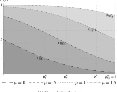
How these two effects unfold is demonstrated in Figures 3–5 for two classes of distributions (and for T = 1): normal distributions N(µ, .5) and power distributions with cumulative distribution functions (CDFs) G(g) = gν (defined for g ∈ [0, 1]). Shown are the CDFs (Figure 3), the detection
function D(p) (Figure 4), and the crime function F(p) (Figure 5) for the different parameter values, where those distributions with higher param-eter values of µ and ν first-order stochastically dominate those with lower values.
Figures 4 and 5 illustrate the trade-off as emerging from proposition 1: when there is large probability mass on low realizations of g (low val-ues of µ and ν), the overall levels of misbehavior and detections are low. But in addition, the value pm where the (hump-shaped) detection function D(p) reaches its peak is small, so that, from corollary 1, the set of
imple-mentable monitoring intensities P1 = [0, pm] is relatively small.
Shifting probability mass to higher realizations of g (that is, increasing
µ and ν) then leads to upward shifts of both F(p) and D(p) since deter-rence is now weaker for any level of p. As a result, pm and hence also the
upper bound of the set P1 increase.16 When there are sufficiently many individuals with large gains from the offense, D(p) may even become monotonically increasing on [0, 1] as in Figure 4A, so that P1 = [0, 1], thereby coinciding with the choice set of the inspector. In this case, con-dition i of corollary 1 is violated; that is, there are many undeterrable in-dividuals, and there is no loss in terms of nonimplementable monitoring intensities, so that theorem 1 has no bite.
Interestingly, with respect to the resulting minimum crime level F(pm), the benefit from a larger choice set P1 due to a larger pm can outweigh the cost in the form of an upward shift of the crime function F(p). For example, for the case of the normal distribution with the monotonically increasing detection function (µ = 1.5) just discussed, there are many
criminals who are not deterred even when monitored with the maximum feasible intensity p = pm = 1 (see Figures 4A and 5A). Therefore, the minimum crime level is F(1) = .84. In contrast, for the power distribu-tions considered, full deterrence is in principle possible as F(1) ≡ 0 for all ν > 0 (see Figure 5B). However, only monitoring intensities p ∈ [0, pm] are implementable, and, as can be seen from Figure 4B, pm < 1 holds. Therefore, the minimum crime level F(pm) might well exceed that result-ing under the monotonic case: for example, for ν = 10, we get pm = .78 < 1, which leads to F(pm) = .91 > .84.
4.2. Varying the Fine
To investigate the impact of changes in the exogenous fine T, it is useful to now express explicitly, where appropriate, the dependency on T; that is, we now write F(p, T), D(p, T), and pm(T). Analogous to the compar-ative statics concerning the distribution G (embodied in proposition 1), changes in the fine T have two countervailing effects on the set of imple-mentable monitoring policies.
Proposition 2. Consider two fines T and T with T < .T
i) For any given monitoring intensity p > 0, the number of detections and the level of misbehavior are smaller under T than under T; that is,
<
( , ) ( , )
F p T F p T and D p T( , ) <D p T( , ).
ii) Let G satisfy conditions i and ii of corollary 1. Then the set of
im-16. For example, consider the case ν = 1 in the power distribution, which corre-sponds to the uniform distribution of gains over [0, 1]. Since m=1
2
p , the crime level is at least m =1
2
( ) .
F p Thus, when the governor wants to deter more than half of the popula-tion (for instance, because the harm from the offense is large), then the required monitor-ing policy >1
2
348/ T H E J O U R N A L O F L E G A L S T U D I E S / V O L U M E 4 5 ( 2 ) / J U N E 2 0 1 6
plementable monitoring intensities is smaller under T than under T. For-mally, P 1 P1 because p Tm( ) <p Tm( ).
Proposition 2.i shows that an increase in T leads to a downward shift of F(p, T) and D(p, T), thereby unambiguously lowering both the number of offenses and the number of detections. Intuitively, for every given p, a higher fine increases the expected penalty from committing the offense and hence leads to fewer offenses and, as a result, fewer detections.
However, analogous to the comparative statics concerning the distri-bution G, proposition 1.ii points to a countervailing effect in the sense that it leads to a smaller set of implementable monitoring intensities P1 = [0, pm(T)]. This result is in contrast to the celebrated finding of Becker (1968), according to which any expected fine pT should be implemented with T as large as possible, as increasing T is costless (in contrast to in-creasing p being costly). For the contexts considered here, this suggests that there is a reduced benefit associated with increasing T in the form of a shrinking set of implementable monitoring intensities. This trade-off is illustrated in Figure 6 for the case in which the gains from crime are distributed according to a standard normal distribution N(0, 1) and for different levels of T. As can be seen in Figure 6, low values of T give rise to a large set of implementable monitoring intensities (that is, pm(T) is large), but the resulting crime level (and the number of detections) is high. A higher value of T reduces the crime level, but it also reduces the set of monitoring intensities that can be implemented by the governor. Which effect dominates depends on whether pm(T)T is increasing or decreasing in T, which in turn depends again on the underlying distribution G. In-terestingly, in the example of the normal distribution depicted in Figure 6, the two effects just balance each other such that the minimum crime level F(pm(T), T) remains constant. For the case of power distributions, this property can even be shown analytically: that is, as long as pm(T) is interior, F(pm(T), T) is independent of T.17 This implies that, in contrast to standard arguments, the minimum crime level cannot be reduced by an increase in the fine T.
17. Indeed, consider F(p, T) = 1 - (pT)ν for pT ≤ 1. Using the first-order condition,
we obtain pm(T) = 1/[(ν + 1)1/νT ], which is interior given that T > (1 + ν)−1/ν. Finally,
350/ T H E J O U R N A L O F L E G A L S T U D I E S / V O L U M E 4 5 ( 2 ) / J U N E 2 0 1 6 5. CRIME-SENSITIVE INSPECTORS
One major implication of theorem 1 is that inspectors cannot be induced to choose monitoring intensities beyond the ceiling pm, which puts a lower bound F(pm) on the resulting crime level. We now investigate to what extent this result relies on the assumption maintained so far that inspectors care only about their remuneration and costs of effort and not about the level of crime itself (see equation [1]). In this section, we relax that assumption and allow for crime-sensitive inspectors, characterized by the more general utility function
b = -b
-( , ) [ ( )] ( ) ( ),
u p R D p F p C p (3)
where β measures how the inspector’s utility is affected by the presence of crime. Thereby, disutility (β > 0) can be caused by intrinsic motivation to
keep the crime level low, while benefits of crime (β < 0) can arise, for ex-ample, from accepting bribes.18 The inspector’s preferences from the basic model are nested as the special case β = 0 in this utility function.
As will be shown, inspectors with a sufficiently strong intrinsic moti-vation can be induced to implement monitoring intensities p > pm, which are not implementable in the basic setup. However, it turns out that for any type of inspector, there is still a potentially large set of monitoring intensities that are not implementable.
To illustrate this point, we set T equal to 1 and consider quadratic costs of effort C(p) = cp2 for some cost parameter c > 0. Moreover, for the sake of analytical tractability, we focus on the case in which the gains from the offense are uniformly distributed on [0, 1], which corresponds to the special case ν = 1 for the power distributions considered in Figure 3, leading to F(p) = 1 - p. The resulting detection function D(p) = p(1 -
p) is then hump shaped and symmetric around m= 1 2
p . Also, the condi-tions of corollary 1 are satisfied, so that the set of implementable moni-toring intensities is = 1
1 [0, ]2
P for an inspector who is not crime sensitive (β = 0). The following result characterizes this set for crime-sensitive
in-spectors (β ≠ 0).
18. The literature discusses other reasons why inspectors might worry about the pre-vailing level of crime, for example, payments that are inversely related to the crime level (Garoupa and Klerman 2002) or a lower tax revenue with part accruing to the enforcer (Coşgel, Etkes, and Miceli 2011). In a different framework, Besanko and Spulber (1989) assume that an inspector can allocate a given budget between enforcement and perqui-sites, so that the marginal rate of substitution can also be interpreted as a measure of the inspector’s concern about crime.
Proposition 3. Let the distribution of gains be uniform on [0, 1] and
T = 1 such that F(p) = 1 - p and m= 1 2
p . Moreover, let the inspector’s utility function be given by equation (3) with C(p) = cp2. When the in-spector’s disutility from crime is sufficiently high (that is, for β > c), then
the set of implementable monitoring policies is 1 2
[ , 1]. Otherwise (that is, for β < c), it is given by = 1
1 [0, ].2
P
The underlying intuition for the proposition is simple: any reward of-fered for the desired number of detections D p( )ˆ can also be gained with mimicking ˆp by choosing p= -1 pˆ instead since D p( ) =D p( ).ˆ It then depends on the inspector’s sensitivity to crime β, in relation to the costs
of monitoring, whether the higher or the lower monitoring intensity is preferred. In the knife-edge case of β = c, the inspector is indifferent
be-tween each pair of monitoring intensities that lead to the same number of detections.
Proposition 3 suggests that inspectors can be distinguished with respect to their β type as follows: For badtypes (β < c), the intrinsic motivation
for curbing crime is low, and we are back to the setting underlying the-orem 1, which renders monitoring intensities p > pm nonimplementable. The resulting crime level tends to be high (that is, larger than F(pm)), and detected offenders should hence be classified as scapegoats.
In contrast, for good types (β > c), the intrinsic motivation is suf-ficiently high such that they can be induced to choose high monitoring intensities. In this case, the number of offenses is low, and the detected offenders should rather be classified as black sheep. Notice, however, that in this case, a mirror result of theorem 1 applies in the sense that only monitoring intensities p ≥ pm can be implemented, and lower ones can-not.
6. LINEAR REWARD SCHEMES
The inspector’s degree of intrinsic motivation also crucially determines his behavioral response to changes in the reward scheme R[D(p)]. We il-lustrate this effect by considering simple linear payment schemes in which for each detection the inspector receives a predefined reward (or bounty)
r; that is, R[D(p)] = rD(p). This specification of payments is employed in
the literature on delegated (private) enforcement (see, for example, Becker and Stigler 1974; Landes and Posner 1975; Polinsky 1980; Besanko and
352/ T H E J O U R N A L O F L E G A L S T U D I E S / V O L U M E 4 5 ( 2 ) / J U N E 2 0 1 6
Spulber 1989). The inspector’s optimal monitoring policy p*(r, β) then satisfies b b Î Î - -[0, 1] *( , ) arg max ( ) ( ) ( ). p p r rD p F p C p
Keeping the parameterizations of Section 5, this leads to the following result:
Proposition 4. Let the distribution of gains be uniform on [0, 1] and
T = 1 such that F(p) = 1 - p, and let the inspector’s utility function be
given by equation (3) with C(p) = cp2. If R[D(p)] = rD(p) with r not too small (that is, r ≥ max{-β, β - 2c}), then
i) the inspector’s optimal monitoring policy is given by p*(r, β) = (r + β)/2(r + c), which is increasing in β, and
ii) an increase in the reward r leads bad (good) types to optimally choose a higher (lower) monitoring intensity; that is, ∂p*(r, β)/∂r > 0 ⇔
β < c and ∂p*(r, β)/∂r < 0 ⇔ β > c.
As for proposition 4.i, more intrinsic motivation to curb crime β leads
to a higher level of monitoring effort.19 Thereby, b > m = 1 2
*( , )
p r p if
and only if β > c, so that indeed each type optimally chooses a moni-toring intensity from the set of implementable ones as characterized in proposition 3.
Proposition 4.ii reveals that the responses of the two types of inspec-tors to changes in the bounty rare quite different: For bad types (β < c),
starting at the lower bound r = -β we have p*(r, β) = 0, and the mon-itoring intensity increases as r increases, approaching b = 1
2
*( , )
p r from
the left in the limiting case r → ∞.20 In this case, higher monetary rewards have the standard effect of increasing the monitoring intensity, generating more detections, and thereby lowering the number of offenses.21
19. In the framework of Coşgel, Etkes, and Miceli (2011), the inspector chooses a higher level of effort when he benefits from a lower level of crime in the form of higher taxation income.
20. This is shown formally at the end of the proof of proposition 4; see also Garoupa and Klerman (2002).
21. In the context of corporate criminal liability considered in Arlen (1994), a firm is required to monitor its employees, and because of vicarious liability, it is liable for crimes committed by them. Liability is triggered (only) when a crime is detected by the firm so that, similar to our framework, the introduction of vicarious liability (which can be in-terpreted as a negative bounty for each detection) may in fact decrease the firm’s optimal monitoring intensity.
In contrast, for good types (β > c), p*(r, β) is decreasing in the reward
r, starting at the lower bound r = β - 2c, where p*(r, β) = 1 and
ap-proaches b = 1
2
*( , )
p r from the right as r increases. Note that these types also respond by generating more detections when the marginal benefit r of doing so increases. However, they achieve more detections by reducing their monitoring intensity, which leads to more offenses. This result is in line with the literature on motivational crowding out in the sense that the inspector’s monitoring effort is lower the stronger the monetary incen-tives (see, for example, Deci 1971; Deci, Koestner, and Ryan 1999; Frey and Jegen 2001; Gneezy, Meier, and Rey-Biel 2011). In our framework, however, this effect is not due to the fact that such incentives directly reduce the inspector’s degree of intrinsic motivation, for example, in the sense of turning a noneconomic relationship into an economic one (see, for example, Titmuss 1970; Frey and Oberholzer-Gee 1997; Gneezy and Rustichini 2000a, 2000b). Rather, for inspectors with a high degree of intrinsic motivation, generating more detections requires a lower moni-toring effort, thereby also leading to more offenses.
The dependence of the inspector’s response to monetary rewards on his degree of intrinsic motivation to keep the crime level low has further con-sequences: for example, in order to implement some desired monitoring in-tensity > 1
2
ˆ ,
p the corresponding bounty is r p( , )ˆ b =(b-2 )/(2pcˆ pˆ-1), which is always positive when the inspector’s intrinsic motivation is suf-ficiently strong (that is, for β > 2c), but r p( , )ˆ b <0 (that is, a payment from the inspector to the governor for each detection) is also possible. This occurs for good types with intermediate degrees of intrinsic motiva-tion (c < β < 2c) and when pˆ >p*(0, )b, that is, when ˆp exceeds the monitoring intensity chosen by the inspector under intrinsic motivation alone (r = 0). In that case, the inspector needs to be punished by a nega-tive bounty in order to increase his effort.
One can also relax the assumption that the fine is fixed at T = 1 and explore how changes in T affect the per-detection reward necessary to in-duce a given implementable monitoring intensity as optimally chosen by the inspector. For r such that the inspector’s choice is interior, we have
b = -b
-ˆ ˆ ˆ
( , , ) (2 )/(1 2 ).
r p T cp T Tp For the case of purely monetary
in-centives (β = 0), this is increasing in T so that higher fines induce higher per-detection rewards. With crime-sensitive inspectors (β ≠ 0), however,
the sign of the effect is ambiguous. Taking the derivative with respect to
354/ T H E J O U R N A L O F L E G A L S T U D I E S / V O L U M E 4 5 ( 2 ) / J U N E 2 0 1 6
whether rewarding the inspector for detections becomes more or less costly for the governor as the fine increases.22
All in all, our findings suggest that payment schemes based on the number of detections such as bounties are delicate instruments that are sensitive to the inspector’s concern for keeping the crime level low. In particular, ignoring an inspector’s intrinsic motivation might lead to se-verely misguided incentives.
7. SOCIAL WELFARE
So far, the analysis has focused on the implementability of a desired mon-itoring intensity ( )pˆ that is assumed to be exogenously given. In this sec-tion we relax this assumpsec-tion and derive ˆp endogenously as the solution to a maximization problem of the governor who can be considered a so-cial planner. This provides us with an efficiency benchmark against which we then compare our results for implementability. In this respect, the un-derlying social welfare function contains the following elements. First, let the society’s harm from crime be hF(p), where h > 0 is a constant harm from each offense. Furthermore, from the inspector’s payoff function (see equation [3]), we include the inspector’s enforcement costs C(p) and his disutility from crime βF(p), while the remuneration R[D(p)] is a transfer payment between the governor and the inspector, which cancels. More-over, the offenders’ gains from the offense are typically included (see, for example, Polinsky and Shavell 2007), but this is not an uncontroversial issue (see, for example, Stigler 1970). For this reason, we use a general specification that nests both possibilities as special cases, so that social welfare is given by b p ¥ ¢ = - + ´ - +
ò
´ SW( ) : ( ) ( ) ( ) ( ) pT p h F p C p g G q dq, (4)where the parameter π ∈ [0, 1] reflects the weight that the social planner puts on the offenders’ gains from the offense.23
22. A special case of a linear reward occurs when the inspector keeps the collected fines; that is, r = T. If interior, the optimal monitoring intensity is then given by p(β, T) = (1 + β)T/(2T 2 + 2c), which is hump shaped in T where the maximum is attained at
= .
T c Hence, for fines beyond this threshold, a higher fine (that is, a higher reward per detection) would induce the inspector to choose a lower monitoring intensity.
23. The special case π = 0 is consistent with an alternative interpretation. If the spector has an outside option of 0 and the governor chooses the reward to satisfy the in-spector’s participation constraint, then R[D(p)] = βF(p) - C(p), such that the governor’s payoff coincides with social welfare defined in equation (4), when setting π equal to 0.
Throughout, we continue with the uniform-quadratic specification; that is, the gains from the offense are uniformly distributed on [0, 1], T = 1 (so that F(p) = 1 - p and m=1
2
p ) and C(p) = cp2. The desired moni-toring intensity ˆp can thus be defined as maximizing the following social welfare function: p b Î é ù ê ú = = - ê + - - ú -ë û 2 [0, 1] ˆ arg max SW( ) (1 ) (1 ) . 2 p p p p p h cp (5)
It is easily seen that social welfare is always strictly concave in p and, given that h + β > 0, also strictly increasing at p = 0 such that the welfare optimum either is attained at the boundary (pˆ =1), which here leads to full deterrence, or is interior.24 In the latter case, it solves the first-order condition SW ( )¢ pˆ =0 and is given by
b p + = + ˆ . 2 h p c (6)
Hence, the efficient (interior) monitoring intensity increases as offenses become more detrimental for the society (h), when the inspector becomes more crime sensitive (β), as the gains from the offense receive less weight in the social welfare function (π), and when the cost of monitoring
de-creases (c).
In a next step, we compare the efficiency benchmark with our previ-ous findings concerning implementability (in particular, theorem 1 and proposition 3). This leads to the following result:
Proposition 5. Let social welfare be given by equation (5) so that the resulting socially optimal monitoring intensity is pˆ.
i) When the inspector’s crime sensitivity is low (β < c; bad type), ˆp is implementable if and only if the harm from the offenses is sufficiently small; that is, h ≤ c - β + π/2. Otherwise, underenforcement arises.
ii) When the inspector’s crime sensitivity is high (β > c; good type), ˆp is implementable if and only if the harm from the offenses is sufficiently large; that is, h ≥ c - β + π/2. Otherwise, overenforcement arises.
The proposition can be illustrated using the taxonomy presented in Table 1. Thereby, p* denotes the (privately) optimal monitoring intensity
24. The socially optimal monitoring intensity is interior for sufficiently large costs of monitoring. More precisely, given that h + β > 0, ˆp is interior if and only if c > (h + β - π)/2.
356/ T H E J O U R N A L O F L E G A L S T U D I E S / V O L U M E 4 5 ( 2 ) / J U N E 2 0 1 6
chosen by the inspector for a given reward scheme R[D(p)]; that is, p* maximizes the inspector’s payoff as given in equation (3).25
As for proposition 5.i, bad types exhibit a low intrinsic motivation to curb crime such that only p* from the set [0, pm] can be implemented (see proposition 3). If the level of social harm from crime is sufficiently low, the welfare-maximizing monitoring intensity ˆp also belongs to this set and hence becomes implementable. For example, it can be shown that by setting a bounty rˆ=[ch-(bp/2)]/[( /2)p - - +h b c], the gover-nor indeed induces the inspector to choose p*= ˆp.26 For greater harm from crime, p*£pm<pˆ holds, which implies that underenforcement is inevitable.
Analogously, in proposition 5.ii the inspector’s intrinsic motivation level is high, so that only high monitoring intensities p* ∈ [pm, 1] can be implemented (see proposition 3). Hence, the welfare-maximizing moni-toring intensity also belongs to this set only when the harm from crime is sufficiently high such that ˆp>pm holds. For low levels of harm from crime, overenforcement arises since pˆ <pm £p*. Note that the condi-tions for overenforcement require that h < π/2 (since we must have β + h - (π/2) < c < β), so that overenforcement can occur only when the
offenders’ gains from the offense also enter the social welfare function (π > 0).
25. Note that there typically exist several reward schemes that lead to the same p. For example, in the proofs of theorem 1 and proposition 3, we consider a simple discontinu-ous reward scheme. But it can be shown that, except for pm (where the detection function D(p) reaches its hump), all implementable monitoring policies can also be reached with a linear reward scheme, as discussed in Section 6.
26. Importantly, in our model there are no restrictions on the feasible transfers be-tween the governor and the inspector (for example, due to limited liability). This implies that in our setup there is no issue with additional distortions because of a trade-off be-tween rent and efficiency, which arises in many agency models (see, for example, Laffont and Martimort 2002) and would affect the possible implementability of ˆp even on the diagonal of Table 1.
Table 1. Privately Optimal versus Efficient Monitoring Intensities
Low Harm from Crime:
p
b
< - +2
h c
High Harm from Crime:
p
b
> - +2
h c
Low sensitivity to crime: β < c p*, pˆ £pm p*£pm< ˆp
Implementable Underenforcement High sensitivity to crime: β > c pˆ<pm£p* p*, pˆ³pm
In terms of this taxonomy, one could argue that the previous literature (see, for example, Polinsky 1980; Garoupa and Klerman 2002; Coşgel, Etkes, and Miceli 2011) confines attention to the cases with low sensitiv-ity to crime in Table 1, while we also analyze the cases with high sensi-tivity to crime.27 We consider both of these novel cases to be empirically relevant. Intrinsic motivation might be one explanation why in many sit-uations where the desired level of monitoring intensity is high there is no issue of implementability, although an inspector’s shirking would not reduce his payments. And intrinsic motivation can cause overenforcement when the governor’s desired monitoring level is low, for example, in the case of minor offenses that are fully deterred by an overly motivated in-spector.
In general, our analysis points to some degree of congruity of the in-spector’s crime sensitivity (β) and the social harm from crime (h), which
is required in order to make the efficient monitoring intensity imple-mentable. This is satisfied on the diagonal of Table 1. Hence, when the level of harm is high, inspectors with strong intrinsic motivation are so-cially desirable in order to overcome the underenforcement issue. In con-trast, when the level of harm from crime is low, inspectors with low levels of intrinsic motivation seem better suited since they do not overenforce.28
It is also interesting to investigate how a change in the fine T would affect these results. While a full analysis is beyond the scope of the paper, it is clear that the following effects need to be taken into account. First, as shown in proposition 2, the monitoring intensity for which the number of detections is maximized becomes smaller as the fine increases (that is,
pm(T) is decreasing in T), which shrinks the set of implementable monitor-ing intensities for inspectors with low levels of intrinsic motivation (bad
27. Indeed, propositions 1 and 5 in Polinsky (1980) refer to high crime and under-enforcement; Garoupa and Klerman (2002) show that there is a linear reward scheme (bounty) that implements a desired monitoring policy under low levels of harm but not high levels of harm; and Coşgel, Etkes, and Miceli (2011) introduce an inspector’s crime sensitivity by the right to collect taxes, but they do not explore the possibility that the disutility from crime is strong enough that the lower cells become relevant.
28. The optimal alignment of preferences in principal-agent settings with delegation is also discussed in contexts other than law enforcement. For instance, Bubb and Warren (2014) study a principal’s optimal delegation decision when agents differ with respect to how strongly they care about the social costs and benefits from a regulatory policy such as environmental protection. They show that it is typically not optimal for the principal to select an unbiased agent (that is, one with the same preferences as the principal with respect to the policy). The reason is that biased agents might have a stronger incentive to engage in information acquisition about new regulatory opportunities.
358/ T H E J O U R N A L O F L E G A L S T U D I E S / V O L U M E 4 5 ( 2 ) / J U N E 2 0 1 6
types). Second, a higher fine changes the threshold for the classification as either bad or good types (now the condition is β ≶ c/T 2 instead of β ≶ c). Third, the fine also affects the welfare-maximizing (interior) monitoring intensity pˆ=[ (T h+b)]/(pT2+2 )c, which is increasing in T as long as the weight of the gains from the offenses in the social welfare function (π) is not too large. Taken together, whether a higher fine increases the scope of implementability of ˆp or instead fosters underenforcement or overenforcement is generally ambiguous and depends on the underlying distributional assumptions as well as on the model’s other parameters. For any given fine, however, one can distinguish cases analogous to those in Table 1 and obtain the corresponding implementability results.
8. DISCUSSION
In this paper, we contribute to the literature on delegated monitoring in which only the number of detections, and not the underlying monitoring intensity or the level of misbehavior, can be observed by the delegating authority (governor). This literature points to a problem of underenforce-ment in the sense that the first-best monitoring intensity need not be im-plementable. The reason is that when several monitoring intensities are observationally identical (that is, give rise to the same number of detec-tions), the inspector to which the monitoring task is delegated can typi-cally be induced to choose only the minimum of these. This also imposes a lower bound on the resulting crime level.
We first generalize the results from the previous literature and charac-terize the full set of implementable monitoring policies. We then perform a comparative-statics analysis to study how the set of implementable monitoring intensities varies with changes in the distribution of gains from the offense and in the fine. This set is small for low benefits from crime or high fines. In particular, the largest monitoring policy that is implementable decreases with the fine such that deterrence need not be increasing in the fine.
We then consider an extension of the model in which the utility of inspectors is directly influenced by the number of offenses in the popula-tion. In this respect, we believe that the intrinsic motivation to keep the level of crime low is an empirically relevant (and commonly neglected) factor. We first show that low levels of intrinsic motivation do not qual-itatively affect the findings from the baseline model, and still only
rel-atively low monitoring intensities can be implemented. However, when the degree of intrinsic motivation is sufficiently large, a mirror result pre-vails, and the set of implementable policies is bounded from below in-stead. Consequently, either the desired monitoring policy is large enough to be implementable or overenforcement occurs; that is, for any payment scheme, the inspector will choose a monitoring intensity that is larger than the one the governor wants to implement.
Our results also suggest that when inspectors are crime sensitive (for example, because of intrinsic motivation), incentive schemes such as bounties as often discussed in the related literature might be even more delicate instruments than previously thought. The reason is that it cru-cially depends on the inspector’s degree of intrinsic motivation whether such extrinsic incentives tend to reinforce the monitoring incentives gen-erated by intrinsic motivation or crowd them out.
Our analysis, hence, points to the potentially crucial role of the de-gree of intrinsic motivation in the context of delegated monitoring, which, however, will typically be unobservable for governors. Therefore, an interesting extension of the model would be a screening framework in which the governor can offer different pairs of monitoring intensities
bˆ ( )
p and payments R( ),bˆ depending on the inspector’s reported type bˆ
(which does not necessarily coincide with his true type β). In contrast to standard screening models, the resulting design problem for the governor becomes significantly more intricate because of additional incentive con-straints. This is due to the fundamental property of this setting in which multiple monitoring intensities give rise to the same number of detections, which increases the scope of mimicking. A full analysis of such an ex-tended screening framework is, however, beyond the scope of the present paper. From a more practical point of view, one possibility for learning about an inspector’s intrinsic motivation over time would be to exploit the different comparative-statics properties of agents with different de-grees of intrinsic motivation. For example, if it is possible to manipulate the costs of monitoring, then good types can be separated from bad types since the number of detections increases in only one of the two cases.
Finally, our analysis also sheds light on which contexts of delegated monitoring are more prone to issues such as under- or overenforcement and the ensuing consequences. In this respect, note that our framework applies not only to the arena of law and economics but in principle also to other settings of monitoring such as enforcing safety and ethical stan-dards in the manufacturing industry or hygienic stanstan-dards in the food
360/ T H E J O U R N A L O F L E G A L S T U D I E S / V O L U M E 4 5 ( 2 ) / J U N E 2 0 1 6
industry. Another relevant context is education, where a school authority delegates the task of educating pupils to schools and teachers. In doing so, it is an outsider in the sense that it can typically observe only which grades are awarded in a school. However, it does not observe whether, for instance, good grades are due to the fact that the school, its teach-ers, and the pupils are all hard working or whether they are the result of a (tacit) agreement among these parties to grade leniently. As a result, looking only at grades might not be very informative about the level of education of pupils or the quality of schools. In this context, however, by featuring state- or nationwide tests that all pupils must take, it seems that authorities have successfully implemented institutional changes to ame-liorate the problem that schools of different quality might be observation-ally identical.29 Even though such or similar measures might not always be available in the contexts to which our framework applies, our analysis nevertheless clearly points to the beneficial role of institutional changes that help authorities overcome their outsiderstatus.
APPENDIX: PROOFS
A1. Proof of Theorem 1
ForpˆÏP1, there is a pÎP1 such that D p( ) =D p( )ˆ by definition of P1. Noting that
=
ˆ
[ ( )] [ ( )]
R D p R D p while C p( ) <C p( )ˆ, it follows that u p( ) >u p( )ˆ, which shows that ˆp cannot be implemented. Now, suppose that pˆ ÎP1. Let ( )= ( )1 +e
d
R d C p
if d=dˆ:=D p( )ˆ and R(d) = 0 otherwise. Then u p( )ˆ = >e 0, while for small enough ε we have u(p) ≤ 0 for all p¹ ˆp because other monitoring intensities p that lead to the same number of detections (that is, pÎPˆd) are associated with
higher costs, and all other choices (that is, pÏPˆd) do not lead to any reward. For the second statement, note that continuous G renders F continuous and thus renders D continuous as well. Since D(p) starts with D(0) = 0 and reaches its global maximum for the first time at pm, D(p) attains every value of its image ∆ in
the interval [0, pm]. Thus, for any d ∈ ∆, Î m 1d [0, ].
p p
A2. Proof of Proposition 1
Consider two distributions G and G, where G is first-order stochastically domi-nated by G; that is, G g( )³ G g( ) for all g. Denote by F p( ) and D p( ) the respective functions resulting under G.
i) For all p ∈ [0, 1], we have
29. In Germany, for example, many states recently introduced mandatory statewide tests in German, English, and mathematics.
Figure A1. Marginal deterrence and detection effects for distributions G and G = - £ - = ( ) 1 ( ) 1 ( ) ( ) F p G pT G pT F p and = - £ - = ( ) [1 ( )] [1 ( )] ( ). D p p G pT p G pT D p
ii) Under corollary 1.i, pm and pm are characterized by the first-order
con-ditions 1 - G(pT) = pTG′(pT) and 1-G pT( )=pTG pT¢( ). By corollary 1.ii, the right-hand sides of both equations are increasing in p. The left-hand sides of both equations are decreasing in p such that pm and pm are the only
inter-sections. This is illustrated in Figure A1 (while the FOSD always implies that
- ³
-1 G pT( ) 1 G pT( ), the relation of the two right-hand sides is ambiguous). Observe that pm³pm if and only if 1-G p T( m )³p TG p Tm ¢( m ). The assumption
¢ - ¢ < -( m ) ( m ) [ ( m ) ( m )]/( m ) G p T G p T G p T G p T p T is equivalent to = ¢ ¢ - m > m m + -m - m m 0 1 G p T( ) p TG p T( ) [1 G p T( )] p TG p T( ), (A1)


![Figure A1. Marginal deterrence and detection effects for distributions G and G = - £ - = ( )1()1() ( )F pG pTG pTF p and = - £ - = ( )[1()][1()] ( ).D ppG pTpG pTD p](https://thumb-eu.123doks.com/thumbv2/123doknet/14808857.610263/31.648.111.560.112.503/figure-marginal-deterrence-detection-effects-distributions-ptg-ptpg.webp)
