Hygrothermal performance assessment of stucco-clad wood frame walls having vented and ventilated drainage cavities

Publisher’s version / Version de l'éditeur:

Advances in Hygrothermal Performance of Building Envelopes: Materials, Systems and Simulations, pp. 198-231, 2017-09-01

READ THESE TERMS AND CONDITIONS CAREFULLY BEFORE USING THIS WEBSITE. https://nrc-publications.canada.ca/eng/copyright

Questions? Contact the NRC Publications Archive team at

PublicationsArchive-ArchivesPublications@nrc-cnrc.gc.ca. If you wish to email the authors directly, please see the first page of the publication for their contact information.

NRC Publications Archive

Archives des publications du CNRC

For the publisher’s version, please access the DOI link below./ Pour consulter la version de l’éditeur, utilisez le lien DOI ci-dessous.

https://doi.org/10.1520/STP159920160100

Access and use of this website and the material on it are subject to the Terms and Conditions set forth at

Hygrothermal performance assessment of stucco-clad wood frame

walls having vented and ventilated drainage cavities

Saber, Hamed H.; Lacasse, Michael A.; Moore, Travis V.

https://publications-cnrc.canada.ca/fra/droits

L’accès à ce site Web et l’utilisation de son contenu sont assujettis aux conditions présentées dans le site

LISEZ CES CONDITIONS ATTENTIVEMENT AVANT D’UTILISER CE SITE WEB.

NRC Publications Record / Notice d'Archives des publications de CNRC: https://nrc-publications.canada.ca/eng/view/object/?id=5da7442c-1281-4b32-8681-03473d9a620c https://publications-cnrc.canada.ca/fra/voir/objet/?id=5da7442c-1281-4b32-8681-03473d9a620c

1

Hygrothermal Performance Assessment of Stucco Clad Wood

Frame Walls Having Vented and Ventilated Drainage Cavities

Hamed Saber1_{, Michael A. Lacasse} 2_{, and Travis Moore} 3

ABSTRACT

The long-term performance in respect to moisture management within any wood frame wall assembly depends on the hygrothermal response of the wall to local climate moisture loads. Estimating the wood moisture content, temperature and time of exposure to conditions suitable for the onset, growth and propagation of mold or rot are critical parameters when assessing the longevity of wood frame structures. A number of approaches to assessing the vulnerability of wood frame structures to deterioration have been developed in recent years one of which has been used by NRC-Construction for evaluating the performance of wall assemblies based on the results from hygrothermal simulation. In this paper, an example of the use of this approach for the assessment of a stucco-clad wall incorporating drainage cavities is described as is the use of a Mould index to capture the risk to the formation of mould in walls. An example is given in assessing the moisture management of a stucco-clad wood frame wall incorporating vented and ventilated drainage cavities for three Canadian locations.

Keywords

drainage components, hygrothermal response, moisture performance, moisture management, stucco cladding, wood frame

Background and Introduction

The information presented in this paper reflects a portion of the work that was completed in assessing the expected hygrothermal performance of stucco-clad wood frame wall assemblies incorporating drainage media [1]. Given that the objective of that project was to assess the hygrothermal performance of wall assemblies incorporating several different combinations of drainage components and sheathing membrane, it was of interest to evaluate the ability of wall assemblies to provide sufficient moisture dissipation through the process of drainage and drying of water from these components when subjected to moisture loads as prevail in specified Canadian climates. More specifically, the climates of interest were those prevalent in coastal areas having a moisture index (MI) [2] greater than 0.9 and less than 3400 degree-days, or MI greater than 1.0 and degree days ≥ 3400. In such climate zones, the 2010 National Building Code of Canada (NBC) requires a capillary break behind claddings of all Part 9 prescribed buildings (i.e. housing and small buildings) [3]. Currently, acceptable solutions to the NBC requirement (§ 9.27) for a capillary break include:

(1) A drained and vented air space not less than 10 mm deep behind the cladding;

(2) An open drainage material behind the cladding, not less than 10 mm thick and with a cross-sectional area that is not less than 80% open;

1_{Heat & Moisture Performance of the Building Envelope Group, Building Envelope and Materials, National Research Council}

Canada, NRC-Construction, Ottawa, ON, K1A0R6, Canada; Hamed.Saber@nrc.ca

2_{Heat & Moisture Performance of the Building Envelope Group, Building Envelope and Materials, National Research Council}

Canada, NRC-Construction, Ottawa, ON, K1A0R6, Canada; Michael.Lacasse@nrc.ca; 0000-0001-7640-3701

3_{Heat & Moisture Performance of the Building Envelope Group, Building Envelope and Materials, National Research Council}

(3) A cladding loosely fastened, with an open cross section (e.g. vinyl, aluminum siding);

(4) A masonry cavity wall or masonry veneer constructed according to NBC § 9.20 (i.e. 25 mm vented air space).

As part of this project, the hygrothermal performance of the proposed alternative solutions for the capillary break, and that incorporated a specific combination of drainage component and sheathing membrane, was compared to the performance of a NBC code-compliant “reference” wall built to minimum NBC

requirements using laboratory testing and modeling activities with the following performance criteria: (1) RHT criterion, and;

(2) Mould index criterion.

Thus if a proposed wall system that incorporated a drainage component and sheathing membrane

combination exhibited a level of performance equal to or better than the NBC-compliant reference wall, it would be deemed an alternative solution to the 2010 NBC requirement for a capillary break and could be used with all presently recognized code compliant Part 9 claddings as an acceptable solution [3].

The hygrothermal performance of wall assemblies incorporating drainage components was assessed against the results obtained from numerical simulation of a NBC code-compliant reference wall assembly when subjected to environmental loads for the selected climate locations in Canada described earlier, and conforming to interior boundary conditions as described in the ASHRAE Standard S-160 [4].

In this paper, information is provided in four sections. The initial section consists of a brief overview of the hygrothermal simulation model, hygIRC-C that was used to complete the simulations. In the subsequent section, summary information is given on all necessary inputs to the simulation model, including brief descriptions of: hygrothermal properties; reference wall configuration; climatic loads acting on walls of a NBC Part 9 building from the wall exterior and those acting on the interior of the wall; water entry through cladding; water drainage and retention in wall assembly; size of drainage gaps of different assemblies incorporating drainage components, and; additional assumptions for completing hygrothermal simulations. Another section provides information on the manner in which performance attributes of specific

components of the wall assembly were defined and on which basis the performance of the code-compliant reference wall was assessed. In the final section, the detailed hygrothermal simulation results for the NBC code-compliant reference wall are provided for three locations having a coastal climate and the results are discussed.

Overview of Hygrothermal Simulation Model, hygIRC-C

The NRC’s hygrothermal model, hygIRC-C, was used to predict the hygrothermal performance within wall assemblies having different drainage components. Results were analyzed on the basis of the risk of moisture-related effects when these walls were subjected to different climatic conditions as might occur across Canada. It is important to emphasize that the predictions by such a model for the airflow, temperature, and moisture (or relative humidity) distributions within a wall assembly, when subjected to a pressure differential (and resulting air leakage rate) across the assembly, are necessary to accurately determine the moisture response in different layers of the wall assembly.

3 were discretized using the Finite Element Method (FEM) as provided in the COMSOL Multi-physics

software package that was used as a solver [5]. The use of the FEM is important as it permits modeling complicated wall geometries with fewer discretizing errors. This simulation model as configured has been extensively used to solve highly complex hygrothermal problems [6, 7, 8, 9, 10]; its response to various physical phenomena has been thoroughly benchmarked and these efforts have been previously described in a number of publications [11, 12, 13].

Description of Wall Assemblies & Hygrothermal Property Characterization

DESCRIPTION OF WALL ASSEMBLIES

Given that the purpose of this project was to assess the hygrothermal performance of walls that incorporated drainage components and thus the component’s ability to provide sufficient drainage and drying to walls subjected to severe coastal climates, the specific requirements given in the NBC are provided in Table 1. Such climates are characterized by a moisture index (MI) greater than 0.9 and with fewer than 3400 degree-days, or MI greater than 1.0 and degree days

≥ 3400; the distribution of locations across Canada having MI > 1 are shown in FIGURE 1. In these regions, the 2010 NBC requires a capillary break behind all claddings of NBC Part 9 construction (i.e. homes and small buildings).

TABLE 1 – 2010 National Building Code requirements for Capillary Breaks in Coastal areas (degree-days < 3400 and MI > 0.9, or degree days ≥ 3400 and MI > 1.0) [3]

Coastal areas

(degree-days < 3400 and MI > 0.9, or degree days ≥ 3400 and MI > 1.0) Sheathing Number of Sheathing

Membranes Capillary Break Part 9 Claddings

NO Sheathing 2 _{10-mm vented air} space (80% open) or drainage material (80% open) or Alternative Solution Lumber siding

Wood shingles & shakes

Fiber cement shingles and sheets(n/a) Plywood

OSB and waferboard Hardboard

Metal siding (horizontal or vertical) Vinyl siding (horizontal or vertical) Stucco OSB/Plywood (Installed but not required) 1 OSB/Plywood (Required and installed) 2

FIGURE 1 – Distribution of locations having MI > 1

The approach used in this project was to compare, on the basis of results derived from hygrothermal simulation, the performance of a reference wall assembly against any other wall assembly incorporating various combinations of wall drainage components and sheathing membranes when subjected to the climate extremes as occur in the coastal regions of Canada. A brief description of the reference wall assembly and one other variation follows.

Reference Wall Assembly

The reference wall assembly was developed based on minimum NBC requirements. Stucco cladding was chosen from amongst the Part 9 claddings (listed in Table 1), as the “worst case scenario” for water penetration. This selection was based on previous work undertaken at the NRC on the moisture management for exterior wall systems [14], in which it was demonstrated that stucco resulted in the highest moisture load behind the primary line of protection, due to its absorptive properties and rain penetration at cracks. The specific code compliant solution for stucco installation considered a solution predominantly practiced on the East Coast, with expanded metal lath (no paper backing) installed on 19 mm strapping; a vertical section of the NBC code-compliant reference wall assembly is shown in FIGURE 2 (i), and in FIGURE 2 (i), a horizontal sectional view. The characteristic drainage component is an air space created by 19 mm plywood strapping installed over on NBC Code-compliant building paper (conforms to CAN-CGSB 51.32).

5

FIGURE 2 – NBC code-compliant reference wall: (i) Vertical section showing stucco installation with capillary break; (ii) Horizontal cross section

The NBC additionally requires the wall to be vented and flashed at the bottom of the wall every

3.5 storeys. Whereas the constructed wall assemblies for the laboratory tests were 1.83 m (6 ft.) in height, subsequent modeling activities took into account the performance of the full 3.5 storey assembly, including the influence of associated rain and wind loads on the hygrothermal performance; this is further discussed in subsequent sections.

A duct penetration detail is included in the assembly drawings. Experimental work in this project examined and quantified the potential for water to enter at a deficiency in the sealant around a duct penetration. This information was then used to determine amounts of water to be introduced in the drainage and drying evaluation of the different assemblies.

HYGROTHERMAL PROPERTY CHARACTERIZATION

To carry out hygrothermal performance assessments of wall assemblies using the numerical simulation tool hygIRC-C, the hygrothermal properties of all materials used for the construction of the different wall assemblies were required as input to the model. Given that a number of the hygrothermal properties of materials of the wall assemblies were available in NRC’s material properties database, only the hygrothermal properties and air flow characteristics of materials that were not available were measured as part of this study. In addition, to permit quantifying the drying potential of various drainage layers, the air flow characteristics of the selected drainage components described were examined; for the reference wall, an empty ventilation cavity of 7 mm depth was characterised for air flow.

A detailed account of the tests methods used to characterise and the resulting values obtained from tests of the hygrothermal properties of wall assembly components and air flow characteristics of the drainage components are given in [15].

GALVANIZED STAPLE

3 COAT STUCCO

EXPANDED DIAMOND-MESH METAL LATH (NO PAPER BACKING) 19 x 38 mm WOOD STRAPPING @ 400 mm o.c. WITH AIR SPACE BUILDING PAPER CAN-CGSB 51.32

11 mm (7/16 in.) OSB SHEATHING BOARD 38 x 140 MM (2 x 6) FRAMING @ 400 mm o.c.

WITH RSI 3.5 (R20) MINERAL FIBRE BATTS 6 mil POLYETHYLENE AIR/VAPOUR BARRIER 13 mm (½ in.) GYPSUM BOARD

DEFINING CLIMATE LOADS ON WALL ASSEMBLY & DRAINAGE SYSTEMS

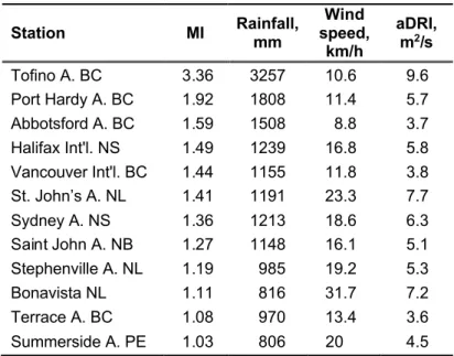
To undertake the hygrothermal simulations, appropriate hourly data for Moisture Design Reference Years (MDRYs) was acquired for the locations identified in TABLE 2. The method used for the MI MEWS project [2] to generate MDRYs was deemed appropriate for use in the current project.

TABLE 2 – List of Canadian locations having MI > 1 Station MI Rainfall, mm Wind speed, km/h aDRI, m2_/s Tofino A. BC 3.36 3257 10.6 9.6 Port Hardy A. BC 1.92 1808 11.4 5.7 Abbotsford A. BC 1.59 1508 8.8 3.7 Halifax Int'l. NS 1.49 1239 16.8 5.8 Vancouver Int'l. BC 1.44 1155 11.8 3.8 St. John’s A. NL 1.41 1191 23.3 7.7 Sydney A. NS 1.36 1213 18.6 6.3 Saint John A. NB 1.27 1148 16.1 5.1 Stephenville A. NL 1.19 985 19.2 5.3 Bonavista NL 1.11 816 31.7 7.2 Terrace A. BC 1.08 970 13.4 3.6 Summerside A. PE 1.03 806 20 4.5

Rankings were produced for all the years in the climate record for each location selected. Three years, wet (maximum), average (median), and dry (minimum), were generated and converted to an acceptable format for hygrothermal analysis. Of these sets, hygrothermal simulations for selected locations were undertaken for an

average (median), followed by a wet (maximum) year. The locations of interest were: St. John’s (East coast

climate – wet and cool, MI = 1.41), Vancouver (West coast climate – wet and mild, MI = 1.44) and Tofino (Extreme coastal climate having MI = 3.36).

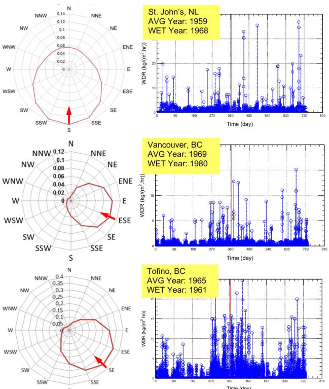
The directional average yearly WDR intensity for St. John’s (NL), Vancouver, and Tofino (BC), are provided in FIGURE 3; the prevailing direction of maximum WDR intensity has been identified for each of these three locations. The prevailing direction of WDR for the West coast locations is easterly, whereas for the East coast location of St. John’s, the WDR is primarily from the southerly direction. The hourly WDR intensity over an “average” year for (a) St. John’s, NL, (b) Vancouver and (c) Tofino, BC is given in FIGURE 4.

The intensity of the maximum average WDR in St. John’s is ca. 0.14 mm/h; in comparison, Vancouver has a similar intensity of ca. 0.10 mm/h, whereas Tofino has a threefold greater maximum average WDR of ca. 0.36 mm/h.

Some additional information regarding climate loads for these three locations is provided in TABLE 3. The average WDR intensity, the total WDR, the number of rain events, and the average outdoor RH (%) are provided for a 2 year period for which the first year was an average year and the second a “wet” year. The data in this table highlight the differences between climate loads used in simulations for these three locations.

7

FIGURE 3 – Directional average yearly WDR intensity: (a) St. John’s, NL; (b) Vancouver; (c) Tofino, BC; shows prevailing direction of maximum WDR intensity

FIGURE 4 – Hourly WDR intensity for (a) St. John’s, NL, (b) Vancouver and (c) Tofino, BC, over an “average” year

0 5 10 15 20 0 90 180 270 360 450 540 630 720 810 Time (day) W D R (k g /( m 2.h r) ) 0 10 20 30 40 0 90 180 270 360 450 540 630 720 810 Time (day) W D R (k g /( m 2.h r) ) 0 5 10 15 20 25 0 90 180 270 360 450 540 630 720 810 Time (day) W D R (k g/ (m 2hr )) St. John’s, NL AVG Year: 1959 WET Year: 1968 Vancouver, BC AVG Year: 1969 WET Year: 1980 Tofino, BC AVG Year: 1965 WET Year: 1961

TABLE 3 – Moisture Index (MI); Average WDR intensity; Cumulative Total WDR; Number of rain events; Average outdoor RH (%) over 2 years (AVG & WET year) for Vancouver, St. John’s and Tofino

Locations

Vancouver, BC St. John’s, NL Tofino, BC

MI 1.44 1.41 3.36

Avg WDR* (kg/m2_{-hr) 0.102 0.139 0.356}

Total WDR (kg/m2_{-hr) 1724 2428 6238}

Number of rain events 2362 1411 2823

Avg annual RH (%) 82 84 89

*Over a 2 year period for which results were obtained for an average followed by a WET year

It is evident that Tofino has the most severe climate with respect to WDR loads, as the cumulative total WDR (6238 kg/m2_{hr) is ca. 2.5 to 3.5 times more severe than that of St. John’s (2428 kg/m}2_{hr) and}

Vancouver (1794 kg/m2_{hr), respectively. This is also reflected by the number of rain events, with Tofino}

(2833) having twice that of St. John’s (1411), but a similar quantity to Vancouver (2362).

The average values for outdoor relative humidity over a 2-year period (average year followed by a wet year) are all in the same order of magnitude for the three locations; however, the highest value is found in Tofino (89% RH), the next highest is St. John’s (84% RH), followed by Vancouver (82% RH). For any of these coastal locations, the ability of moisture to dissipate from wetted wall assemblies is limited by the capacity of the ambient air to absorb moisture, which is more difficult in climates having higher average relative

humidities.

RESPONSE OF WALL ASSEMBLIES & DRAINAGE SYSTEMS TO CLIMATE LOADS

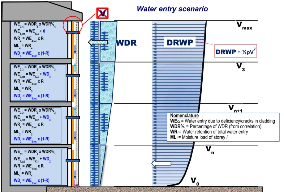
To permit estimating the hygrothermal response of wall assemblies to wind-driven rain (WDR) loads and prevailing climate conditions, there is a need to quantify the amount of water that might enter behind a cladding in relation to the WDR loads that impinge on the wall and as relates to the variation of these loads to the height of the building; this is a required initial step that perhaps can best be visualised in the water entry scenario postulated FIGURE 5. From this illustration the quantity of water entering behind the cladding at any given storey is dependent on determining:

 Wind-driven rain loads acting on the exterior cladding;

 Water entry behind cladding due to water permeation of the cladding and entry at deficiencies;  Water drainage from and retention within a drainage system;

 Moisture loads in drainage cavity at given storey heights  Distribution of moisture loads within drainage cavity Each of these is elements is discussed in turn.

FIGURE 5 – Schematic illustrating WDR and DRWP loads acting on the cladding to bring about water penetration within and water entry behind the cladding

WDR

V

V

V

V

V

DRWP

DRWP = ½ρV

Water entry scenario

V

WECi= Water entry due to deficiency/cracks in cladding

WDR%i= Percentage of WDR (from correlation)

WRi= Water retention of total water entry

From climate loads to wind-driven rain loads acting on wall assembly and cladding

The scenario considered in estimating the hygrothermal response of wall assemblies and drainage systems to climate loads is provided in FIGURE 5, which includes an illustration of the wind-driven rain (WDR) and driving-rain wind pressure (DRWP) loads acting on the walls.

The DRWP acts along the full height of the wall assembly and changes in relation to the height above ground level according to the relationship:

= , < < (1)

Where:

= speed of the wind during rain event at height = gradient wind speed at gradient height (i.e. 10 m)

= exponential coefficient (value from 0.27 (suburban terrain) to 0.60)

The rate at which driving rain is incident on an unobstructed imaginary wall surface can be calculated from the rainfall rate and wind speed using empirical relationships between rainfall rate and drop size distribution [16] and drop size and terminal velocity [17], as expressed in Equation (2):

WDR _{= cos(Θ − 90)} (2)

Where:

= wind speed against the wall in m/s;

= horizontal rainfall intensity in mm/hr; and = wind direction.

As such, and given the increase in wind speed with height, the WDR intensity varies as the height of the building as illustrated in FIGURE 5.

Water entry behind cladding due to permeation of cladding and deficiencies

Water entry to the drainage system behind the cladding may come about due to water permeation through the cladding itself, or through imperfections at the periphery of cladding penetrations such as at ventilation ducts, pipes or windows. Thus at each story, water may enter to the drainage system located behind the cladding through the cladding or through deficiencies at through-wall penetrations.

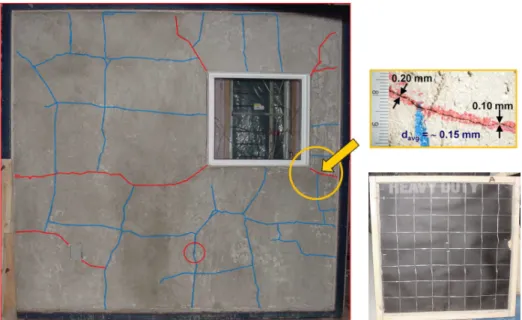
The amount of water that might enter, for example, a stucco clad wall assembly, a photo of which is shown in FIGURE 6, was determined through experimental testing, where a stucco wall assembly was subjected to varying simulated WDR conditions. This entailed spraying the cladding of a 2.44 m by 2.44 m (8-ft. by 8-ft.) test specimen with water over a range of spray rates whilst simultaneously subjecting the wall to pressure differences. Over the course of the water penetration test, water that entered cracks and openings in the cladding, permeated through these deficiencies and thereafter was collected to the drainage system [18]. The percentage of water entry behind a stucco cladding as a function of water deposited on the cladding (L/min-m2_{) and pressure difference(Pa) acrossthe wall asembly is provided in FIGURE 7. A similar set of}

information was derived for the percentage of water entry at through-wall penetrations and this is likewise shown in FIGURE 7.

11

FIGURE 6 – Stucco cladding subjected to water penetration tests

FIGURE 7 – Water entry correlations for entry from (i) permeation of stucco cladding and (ii) deficiencies at through-wall penetrations

0 1 2 3 4 5 6 7 8 0 100 200 300 400 500 600 700 800 3.4 L/(min-m2₎ 1.6 L/(min-m2₎ 0.8 L/(min-m2₎

Low-, Mid- and High-Rise Buildings

Low-Rise Buildings Pressure (Pa) P e rc e n ta g e of W a te r E n tr y (% ) 0 0.02 0.04 0.06 0.08 0.10 0.12 0.14 0.16 0.18 0 100 200 300 400 500 600 700 800 900 1000 1100 1200 1.74 L/(min-m2₎ 1.16 L/(min-m2₎ 0.58 L/(min-m2₎ Pressure (Pa) P e rc e n ta ge o f W a te r E n tr y R at e (% )

Correlations [1] were developed for low-rise buildings for the percentage of water entry in relation to the water deposition rate (WDR) and pressure difference ( ). For water entry behind a stucco cladding, , this is given by:

= 2.54 − 4 X 10 . _{+ 6.2 − 5} . _{, 0 ≤ ≤ 160 (3)}

Whereas, for water entry of deficiencies of through-wall penetrations, _{, such as a ventilation duct, this is} given as:

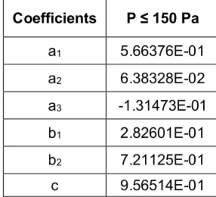
= ∑ + , ≤ 150 , (4)

Where:

= Water entry through deficiencies (mL/min); WDR = Wind driven rain (L/min-m2_{), and;}

= Wind pressure (Pa);

And for which the values of the coefficients, , , and in Eq. (4) are given in TABLE 4.

TABLE 4 – Values of correlation coefficients for Eq. 4 Coefficients P ≤ 150 Pa a1 5.66376E-01 a2 6.38328E-02 a3 -1.31473E-01 b1 2.82601E-01 b2 7.21125E-01 c 9.56514E-01

Water retention in respective drainage systems

Tests were also carried out to characterise the drainage-retention of different drainage systems. The depths of drainage cavities for all the drainage systems were first determined from the construction of stucco clad mock-ups in accordance with the respective specifications of each of the wall assemblies as provided to which NBC-compliant stucco was applied. The work was undertaken by professedly knowledgeable and

experienced stucco contractors. After curing for 28 days, the specimens were then cut at the centre vertically and horizontally so that the interior gaps could be measured to estimate the cavity depth, as seen in

13 The results obtained for the reference wall having a nominal cavity depth of 10 mm was 7 mm of depth derived from measurement of the digitized profile of the reference wall cavity; this cavity depth was used in the numerical simulations and for the fabrication of drainage-retention test specimens. In instances where the measured depth was larger than the nominal depth, the nominal cavity depth was used in the numerical simulations and for the fabrication of drainage-retention test specimens.

After determining the cavity depths for the wall configuration, test specimens were constructed to determine the drainage and retention characteristics of each drainage system. Test specimens of 1220 mm in width by 1830 mm height (4ft. by 6ft.) were dosed with water to the drainage cavity for one hour and across the entire width (i.e. 1220 mm) at constant rates of 3, 4, 5, 6 and 8L/hour. The dosage levels were determined from maximum water entry rates that could occur in selected Canadian locations as provided in [2]. The quantities of water that drained from the system were monitored gravimetrically during the test, and were used to determine the retention rate of the drainage system. The drainage-retention relation was based on the percentage of water that remained in the cavity for a given water entry rate given in mL/h-m2_.

The results of the drainage-retention tests [18] for all drainage systems evaluated are shown in FIGURE 9. The results show that a smaller proportion of water was retained at higher dosage rates deposited to the cavity, whereas a greater proportion was retained for lower dosage rates.

FIGURE 9 – Driange-retention test results for reference and all Client drainage systems

Moisture loads in drainage cavity at given storey heights

Having determined the water entry rates to the drainage systems on the basis of correlations developed for WDR rain loads acting on the cladding and having assessed the quantity of moisture that might drain from a cavity given the dosage to the cavity, the moisture load within the cavity was then estimated for each storey level.

Referring to the schematic provided in FIGURE 5, and taking into consideration the WDR loads as provided from Eq.2 and the percentage of these loads that enter the cavity of the drainage system as provided from both Eq. 3 and Eq. 4, the moisture load (ML) at any given story height, i, is given by:

Moisture load (at storey height, i ) = MLi= WRi (5)

Where:

MLi= Moisture load of storey i

WRi= Water retention of overall water entry at storey i = WEi,tot x R (6)

And where:

R = % retained in the drainage system and 1-R = % water drained from system

WEi,tot= total quantity of water entry at storey i = WEC,i+ WDi+1 (7)

WDi= Water drainage from the storey above = WEi,tot x (1-R) (8)

WEC,i= Water entry through cladding and from deficiencies to the drainage system

Also:

WEC,i= WDRix WDR%i (9)

WDR%i= Percentage of WDR (from correlations given in Eq. 3 and Eq. 4)

WDRi= Wind-driven rain load at story i (as given by Eq. 2)

The moisture loads within the drainage cavity for each storey height are shown in Error! Reference source

not found.. It follows from this that the ML at the fourth storey differs from that of the other three storeys

given that the total quantity of water entry at this storey is:

WE4,tot= WE

C,4+ 0 (10)

Where in Eq. 10, that portion of water that drains from the storey above, WDi= 0 and as such, the total

quantity of water entry to the drainage system at this storey is simply the percentage of WDR that enters from permeation of water through the cladding and through deficiencies, as provided in in Eq. 3 and Eq. 4.

Distribution of moisture loads within drainage cavity

The manner in which moisture loads within a cavity were distributed depended on the presence of a nominal capillary break, as might be assumed for those drainage systems having cavity depths of at least 10 mm, as illustrated in FIGURE 10.

15 In these instances, the ML was applied to the backside of the cladding if there was a clear cavity, or when the drainage cavity included a drainage component, it was assumed that 50 % of the ML remained on the

backside of the cladding whereas the remaining 50% found its way to the surface of the sheathing membrane. It was surmised that in the case of a clear cavity, the capillary break would prevent any substantial ML from reaching the sheathing membrane, whereas in the presence of a drainage component, it was supposed that there was an equal risk that the ML would remain on the backside of the cladding, or percolate to the surface of sheathing membrane over a storey height. In instances where the nominal drainage system cavity depth was 2 to 4 mm in depth (FIGURE 10; ii), it was assumed that all of the ML reached

the sheathing membrane. This was deemed a plausible scenario given that any water that would permeate the cladding would find its way to the drainage space at fastener locations and thus quickly occlude the interstitial space of these drainage systems given the number and schedule of fasteners used to secure stucco cladding to the frame, as illustrated in FIGURE 10 (ii).

Initial conditions of hygrothermal simulations

The initial temperature in all layers of the wall assemblies were taken equal to 21°C and the initial moisture content of all material layers corresponded to a relative humidity of 50%. Simulations were started on the first day of the month of January of the average climate year for the specified locations.

Defining Performance Attributes

Information in this section describes how performance attributes of specific components of the wall assembly were defined and how the performance of the code compliant reference wall was assessed in relation to the client wall assemblies incorporating drainage components. The locations that were of interest in assessing the performance of wall assemblies are also defined.

LOCATIONS OF INTEREST WITHIN WALL ASSEMBLIES TO ASSESS PERFORMANCE

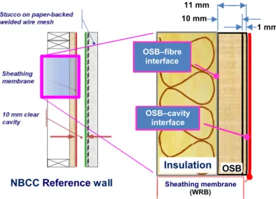
Within the wall assembly there are locations that are of interest given that these may be prone to moisture uptake. Given sufficient temperature conditions and an adequate gestation period, this may lead to the risk of formation of mould or, in the case of wood-based components, wood rot fungi. These locations have been identified in FIGURE 11. In this figure, a schematic of a vertical sectional view of the reference wall assembly is given with a portion expanded to better illustrate the different layers within the assembly. The layers include the sheathing membrane, the sheathing panel (OSB), and the insulation within the stud cavity of the wall. Focus is placed at these locations, as it is at these locations that the risk to the formation of mould or wood rot is heightened given their proximity to the sheathing membrane and drainage cavity where the moisture loads have been applied.

Accordingly, emphasis has been placed on determining the local temperature and relative humidity conditions, which result from simulating the response of the wall assembly to selected climates, at the following four (4) locations in the wall section:

 Interface between the exterior surface of the sheathing panel (OSB/gypsum board) and cavity  Exterior portion of sheathing panel of depth 1 mm

 10 mm portion of sheathing panel (remaining portion of 11 mm panel)

 Interface between the interior surface of the sheathing panel (OSB/gypsum board) and fibrous insulation.

FIGURE 11 – Locations of interest within wall assemblies in assessing relative performance

PERFORMANCE CRITERIA

Two (2) performance criteria were used to assess the performance of wall assemblies. These include the: (i) RHT index, as was used previously in other projects for which the performance of wall assemblies was sought [10, 14], and; (ii) the Mould Index developed by Hukka and Viitanen [19], Viitanen and Ojanen [20], and Ojanen et al. [21]. Both of these criteria is described in turn.

RHT Index

The RHT index is a measure of the risk of formation of mould on surfaces or wood rot of wood-based components given the relative humidity and tempeature profile over a specified time period over which the index is used. The value of the index increases monotonically and thus represents at the end of the period, the maximum cumulative value of the index. The value of the index is given by the following relation:

( ) = ∑ [ − ( )][ − ( )] (11)

Where:

( ) = Cumulative value of the RHT index

( ) = User defined threshold value for relative humidity (RH) ( ) = User defined threshold value for temperature, T (= 5°C)

= total number of 10 day intervals over a simulation period (= 37 / 1 year)

Ther value of the index is detremiedn where the relatrive humidity (RH %) and tempeature (T°C) data are averaged every 10 days over a period; thus, n, in Eq. 11 is the total number of 10 day intervals over a simulation period or 37 for every simulation year of interest. If the user defined threshold value for temperature is 5°C, then the value of the index, as given by Eq. 11, accumulates only when the temperature exceeds 5°C, and when the value of RH is likewise above a given threshold value, as is shown in Error!

Reference source not found..

User defined threshold values for relative humidity % have in previous work been chosen at 80, 90, 92 and 95, depending on the technical requirements. For example, one might have interest in gaining insight on whether the wood-based components are at risk to attaining critical moisture content where wood rot may be initiated.

NBCC Referencewall 1 mm 10 mm OSB OSB–fibre interface OSB–cavity interface Insulation Sheathing membrane (WRB) 11 mm

17 In this project, values were generated for RHT indices of RHT(80), RHT(85) and RHT(92).

Mould Index

The development of the mould index has been on-going for several years with the most recent work, as was used in this project, having being provided by Ojanen et al. [21]. A description of the mould index levels as relate to growth rates is provided Error! Reference source not found., whereas the mould growth sensitivity classes for specified materials and corresponding minimum levels of relative humidity needed for mould growth are provided in Error! Reference source not found.. The mould index levels range in value from 0 to 6, with 0 being equivalent to no growth and 6 indicating 100% coverage of either heavy or tight mould growth. The visual identification of mould growth on surfaces is given an index value of 3. As provided in Error! Reference source not found., the sensitivity of different construction materials to the formation of mould growth was classified in four (4) classes, namely: very sensitive, sensitive, medium resistant and resistant. The assumed correspondence of sensitivity class for materials located within a wall assembly as modelled in this study is given in Error! Reference source not found.. More specifically, the sensitivity class for the sheathing panel (e.g. OSB) was considered “Sensitive”, whereas the sensitivity class of materials in the cavity insulation (i.e. fiber-based insulation) was considered “Medium Resistant”. Only the “Sensitive” mould growth sensitivity class was considered when a comparison was made amongst the relative performance of the respective wall assemblies.

TABLE 5 - Description of Mould Index (M) levels [] M Mould Index (M) - Description of Growth Rate

0 No growth

1 Small amounts of mould on surface (microscope), initial stages of local growth

2 Several local mould growth colonies on surface (microscope)

3 Visual findings of mould on surface, < 10% coverage, or < 50% coverage of mould (microscope)

4 Visual findings of mould on surface, 10%–50% coverage, or > 50% coverage of mould (microscope)

5 Plenty of growth on surface, > 50% coverage (visual)

6 Heavy and tight growth, coverage about 100%

TABLE 6 - Mould growth sensitivity classes and some corresponding materials [20]

Sensitivity Class Materials RHmin(%)*

Very Sensitive Pine sapwood 80

Sensitive Glued wooden boards, PUR with paper surface, spruce 80

Medium Resistant Concrete, aerated and cellular concrete, glass wool, polyester wool 85

Resistant PUR with polished surface 85

* Minimum relative humidity needed for mould growth

TABLE 7 - Mould growth sensitivity classes for different materials of wall assemblies

Sensitivity Class Layers within Wall Assemblies RHmin(%)*

Very Sensitive 80

Sensitive Top plate, bottom plate, OSB, foam 80

Medium Resistant _{Fibre, gypsum, membranes 85}

Resistant 85

Comparison of RHT Index to Mould Index

A comparison between the limits of applicability of the RHT index to that of the mould index for the “sensitive” and “very sensitive” class of materials is shown in FIGURE 12. The risk to mould growth as determined by the RHT index, is delineated by a rectangular pattern ranging, on the temperature scale, between 5 to 30°C and from 100 % RH down to respective threshold values for the selected RHT (x) index (i.e. RHT(80); RHT(85); RHT(92); RHT(95)). Whereas in the case of the mould index, the area for risk to the formation of mould has been identified in red and in blue in instances where there is no risk to mould

growth.

FIGURE 12 - Comparison between the limits of applicability of the RHT index to that of the Mould index; Very sensitive and sensitive class having minimum RH 80%

As is perhaps evident, the RHT index most closely matching that of the mould index is RHT(80) and this is not surprising given that the minimum relative humidity needed for mould growth to “sensitive” and “very sensitive” class of materials is 80% RH. There is as well, deceasing degrees of correspondence between the two mould growth risk indices as the RHT(x) index increases with the least equivalence for the RHT(95) index.

The performance attributes of the selected locations within the wall assembly in this paper are provided at three levels of RHT(x) index (i.e. RHT(80); RHT(85); RHT(92)). Whereas in respect to the mould index, for materials considered as “sensitive” class both the average and maximum values for the mould index have been provided for the respective locations in the wall as identified in FIGURE 11.

Results Derived from Hygrothermal Simulation

A comparison of simulation results over 4 storeys is first described, with all subsequent results provided only for the storey for which the response of the wall assembly is the most significant. The comparison is made on the basis of the mould index (risk to mould growth) or RHT index (risk to the growth of wood rot fungi).

75 80 85 90 95 100 0 5 10 15 20 25 30 Temperature, T (o_C) C rit ic al R e la tiv e H u m id ity , R HC ri t (% )

Risk of Mould

Growth

No Risk of Mould

19 for wood components as “sensitive” (S); the values for RHT index performance are provided for RHT(80), RHT(85), and RHT(95).

COMPARISON OF SIMULATION RESULTS OVER 4 STOREYS (TOFINO, MI = 3.4)

A comparison of results from simulation of the wall response to local climate loads in three Canadian locations (provided above) and for each of 4 storeys is given in FIGURE 13, Table 8 and Table 9. The differences in wall performance as measured by either the mould index or RHT index values for the

respective storeys is not clearly evident from the information provided in FIGURE 13. However, the values for RHT index reported in Table 8 show that the 4th_{storey is the storey with the greatest value of RHT index.}

Accordingly, all subsequent values for performance derived from simulation are reported for the fourth and upper-most storey. The corresponding values for the mould index response of a 1 mm thick sliver of OSB of the 4th_{storey reference wall are given in Table 9, together with the other values for mould index for other}

portions of the OSB panel or at its interface with insulation.

REFERENCE WALL SIMULATION - MOULD INDEX PERFORMANCE

A comparison in mould index response amongst different locations within the wall is first provided followed by results on the response within the wall for selected climate locations.

Comparison in mould index response amongst different locations within wall

The results are first provided with respect to variations in values of mould index for the simulated response of the 4th_{storey reference wall over a 2-year simulation period (in days) for the specified locations within the wall}

(i.e. OSB Sliver; Back of OSB; Whole OSB; OSB-Fibre Interface) and in respect to the three (3) locations for which simulations were completed; this is shown for Tofino, BC, in Figure 14, for Vancouver, BC in Figure 15 and in Figure 16 for St. John’s, NL.

TABLE 8 – RHT index response of Reference Wall (OSB 1 mm thick sliver)

Storey RHT(85) RHT(92) RHT(95)

4 3015 435 37

3 2972 419 33

2 2912 399 28

1 2864 389 26

TABLE 9 – Mould index response of Reference Wall (OSB 1 mm thick sliver)

Layer or Interface OSB Sliver (1 mm) Back OSB (10 mm) Whole OSB (11 mm) OSB-Fibre Interface Avg 3.910 2.506 2.597 1.819 Max 4.508 3.475 3.538 2.984

FIGURE 13 - Comparison of simulation results over 4 storeys for Tofino, BC (MI = 3.4)

0 1 2 3 4 5 6 0 90 180 270 360 450 540 630 720 810 4th Storey 3rd Storey 2nd Storey 1st Storey Time (day) M ou ld In de x, M

The values for mould index performance are based on a mould index sensitivity class “Sensitive” (S) for wood components. Information in tabular form in the respective inserts provides the average and maximum values of mould index attained for the different locations within the wall section over the 2-year simulation period. As is evident from the information provided in tabular form, the greatest value for mould index performance is attained within the 1 mm sliver located at the exterior extremity of the OSB sheathing panel irrespective of the climate location for which simulations were completed.

The average and maximum mould index values for the “OSB sliver” were greatest in Tofino

(i.e. = 3.9; max ( ) = 4.5), and thereafter, in descending order, in Vancouver ( = 3.5; max ( ) = 4.3) and St. John’s ( = 3.1; max _{( ) = 4.2). As such, the mould index values correlate} with the respective values for Moisture index for each climate location.

Reductions in values for mould index during the 2-year simulation period are less pronounced in milder climates as compared to colder climates. For example, the colder climate of St. John’s (HDD = 4800) offers significant reductions in mould index values (Sliver: = 4 to = 3; OSB-fibre interface: = 2 to ~ 0.2 over the winter months (i.e. from day 360 to day 450), whereas for the milder climates of Vancouver (HDD = 2950) and Tofino (HDD = 3150), the reductions in MIDXare much less pronounced.

Layer or Interface OSB Sliver (1 mm) Back OSB (10 mm) Whole OSB (11 mm) OSB-Fibre Interface Avg 3.500 2.181 2.271 1.518 Max 4.270 3.082 3.149 2.633

Figure 14 – Mould index for specified locations in wall assembly as a function of time over a 2 year simulation period for Tofino, BC

Layer or Interface OSB Sliver (1 mm) Back OSB (10 mm) Whole OSB (11 mm) OSB-Fibre Interface Avg 3.910 2.506 2.597 1.819 Max 4.508 3.475 3.538 2.984

21 Layer or Interface OSB Sliver (1 mm) Back OSB (10 mm) Whole OSB (11 mm) OSB-Fibre Interface Avg 3.085 1.941 2.035 1.147 Max 4.210 3.191 3.261 2.562

Figure 16 – Mould index for specified locations in wall assembly as a function of time over a 2 year simulation period for St. John’s, NL

Comparison in mould index response within wall for selected climate locations

The results derived from hygrothermal simulation of the 4th-storey reference wall for each of three selected locations in Canada over a 2-year simulation period (in days) with respect to the mould index (MIDX) performance values are provided for the 1 mm thick sliver of the OSB sheathing panel in FIGURE 17, the back of the OSB panel in Figure 18, the “whole OSB panel in 19, and in Figure 20, the interface between the OSB panel and fibrous insulation.

Mould index values for 1 mm “Sliver”(FIGURE 17) — The mould index values (MIDX) for a

1 mm “Sliver” at the exterior face of a OSB panel of a 4th-storey wall located in Tofino, generally increases over the simulation period, although there is a long period in the initial simulation year where the value of

MIDXremains stagnant at a value of ca. 3.6. The response for Vancouver is similar to Tofino, but less severe. For Vancouver, the maximum value for MIDXattained after 2-years of simulation is ca. 4.3 whereas for Tofino it is 4.5. In the case of the simulated response of the reference wall located in St. John’s, the colder climate retards the growth of the MIDXand provides for a reduction in the MIDXvalue with the onset of the second winter period; thereafter, it attains a maximum similar in value to that obtained for Vancouver.

Mould index for the “Back” 10 mm portion of OSB panel(Figure 18) — The mould index values (MIDX) for the “Back” 10 mm portion of the OSB panel of a wall located in Tofino gradually attains a maximum valve for MIDXover the 2-year simulation period of 3.5; a similar pattern of gradual increase in MIDXis evident for Vancouver, although the maximum for MIDXover the 2-year simulation period is 3. For the colder climate of St. John’s, the simulated response of the reference wall, again, is retarded in the initial simulation months, but does achieve a MIDXvalue of ca. 2.8 in about the ninth month of simulation, only to be reduced over the coming winter months to values of ca. 1.5; thereafter, there is a steady increase again over the subsequent nine months to attain a maximum of ca. 3.2 for this climate location.

Mould index for the “Whole” 11 mm portion of OSB panel(19) — The mould index values (MIDX) for the “Whole” 11 mm portion of OSB panel of a wall at the 4th_{-storey for the selected climate locations is}

OSB Sliver

(1 mm thick) Tofino Vancouver St. John’s AverageMIDX 3.910 3.500 3.085

MaximumMIDX 4.508 4.270 4.210

OSB insulation

interface Tofino Vancouver St. John’s AverageMIDX 1.819 1.518 1.147

MaximumMIDX 2.984 2.633 2.562

23

Mould index for interface between OSB panel and fibrous insulation(Figure 20) — The mould index values (MIDX) for the interface between the OSB panel and the fibrous insulation within a wall section at the 4th_{-storey are reduced as compared to the values obtained at the back or for the entire portion of OSB}

achieving a maximum value for MIDXof ca. 3 for Tofino and ca. 2.6 for either Vancouver or St. John’s. This is simply due to lower moisture contents of the OSB at this location in the wall as compared to locations in the OSB closer to the source of the moisture load.

There is a more pronounced effect of the colder seasons on the mould index values as is evident from the lag in accumulation of MIDXvalues for the initial stages of the simulation and the reduction in MIDXvalues at the onset of the second as well as the subsequent fall-winter season. Of the three climate locations, this effect is most prominent for St. John’s, the coldest of the three climates (i.e. 4800 HDD for St. John’s as compared to 3150 and 2950 for Tofino and Vancouver, respectively).

RESULTS FOR REFERENCE WALL SIMULATION - RHT INDEX PERFORMANCE

The results derived from simulation for the response of the reference wall in terms of the RHT index and subjected to the climate of Tofino over a 2-year simulation period (in days) are shown in Figure 21. In this figure, a relative humidity (% RH) and temperature (°C) plot is provided for the 2-year simulation period for a 1 mm “sliver” of the exterior surface of an OSB panel within a section of the reference wall. The cumulative values for RHT indices achieved after the 2 year simulation are given in the adjoining insert and for which the values for RHT(80), RHT(85), and RHT(92) are provided. The lower the RH threshold value, the higher the value of the corresponding RHT index.

TABLE 10 – Values of RHT index for Selected climate locations

Figure 21 – Relative humidity (%) and temperature (°C) plot over a 2-year simulation period for a 1 mm “sliver” of OSB panel within a section of the reference wall of 4th_{-storey and subjected to Tofino climate}

Similar values have been provided for the respective RHT indices for Tofino (MI = 3.36), Vancouver (MI = 1.44) and St. John’s (MI = 1.41) in Error! Reference source not found.. The severity of the Tofino climate is evident from a review of the values for RHT; Tofino has the highest RHT index value for each of the respective indices. As well, it is difficult to distinguish between the severity of the climate in Vancouver and St. John’s given that the RHT(92) index value for these locations is essentially the same. However, one is able to obtain more discerning index values from the RHT(85) and RHT(80) indices.

DISCUSSION OF SIMULATION RESULTS

The discussion of simulation results focuses on two aspects:

 Trends in response of the reference wall to the three climates to which the walls were subjected;  Location within the section of the wall for which values of MIDXare provided.

Response of reference wall to different climate locations

The most severe location, based on average and maximum values for MIDX, was Tofino, BC. Average values for

MIDX for the OSB panel “sliver” for Tofino were 3.9 as compared to 3.5 for Vancouver and 3.1 for St. John’s; values for max{MIDX} for Tofino, Vancouver and St. John’s, were respectively, 4.5 (+15%), 4.3 (+23%) and 4.2 (+36%); the values in parentheses provide the % increase from the average values. This trend is the same for values reported as an RHT index irrespective of whether the index was RHT(80), RHT(85) or RHT(92).

Variation in values of MIDXfor location within wall section— In general, for any given climate location,

the average and maximum values for MIDXare greatest for locations in the wall assembly closest to the source of the moisture load and decreases as the gap between the moisture source and the location of interest increases. Thus, for example in Tofino, the “sliver” of OSB panel has the greatest average value for MIDXat 3.9, followed by the back portion of the OSB panel (MIDX= 2.5) and thereafter, the interface between the OSB and fibrous insulation (MIDX= 1.8).

The onset for mould growth on or within the OSB panel for any given location is thus more evident for the sliver as compared to the interface between the OSB and fibrous insulation. In Tofino, for example, the onset for mould growth for the 1 mm thick OSB panel “sliver” occurred after the first 15 days whereas this was 120 days for the interface between the OSB and fibrous insulation.

Conclusions

In this report, information has been provided regarding the inputs required to complete hygrothermal simulations and included the following:

 A summary description of the reference wall assembly  Hygrothermal property characteristics

 Defining climate loads for several Canadian location’s including information on the moisture index, annual driving rain index, rainfall, rainfall intensity and prevalent wind-driven rain direction and identification of “average” and “wet” years

 Selection of representative Canadian climate locations for simulation

 Defining the moisture loads acting on components within the wall assembly in consideration of the amount of water entry to and drainage from wall assemblies

25 In addition, a brief overview of the hygrothermal simulation model hygIRC-C has been provided and as well, references have been given on exercises undertaken to benchmark the model.

Finally, results from hygrothermal simulation have been presented in which the response of the reference wall to climate conditions of Tofino (BC), Vancouver (BC), and St. John’s (NL) have been described. The results, as provided by information on the mould index and RHT index within the assembly, permitted comparisons of the response of the reference wall to the different climates. As such, Tofino was deemed to have the most severe climate of the three locations with the least onerous being St. John’s. The colder climate of St. John’s was found to attenuate the response of the wall as evident from the reduced values of moisture index for this location as compared to that of either Vancouver or Tofino.

Acknowledgements

The authors of this paper wish to extend their thanks to the Air Barrier Association of American (ABAA) for having managed and arranged support for this project and in particular, to

Mr. Laverne Dalgleish for his highly proficient handling of all technical and non-technical issues that arose over the course of the project. Our thanks are also extended to NRC-Construction for partial funding of this project and as well our colleagues within NRC-Construction for their technical support, advice, and feedback during the course of this project and who helped support the work described in this report including: K. Abdulghani, M. Armstrong, S. Bundalo-Perc, S. M. Cornick, B. Di Lenardo, G. Ganapathy, W. Maref, P. Mukhopadhyaya, M. Nicholls, M.C. Swinton and D. Van Reenen.

References

[1] H. H. Saber and M. A. Lacasse (2015) Performance Evaluation of Proprietary Drainage Components and Sheathing Membranes when Subjected to Climate Loads – Task 6 – Hygrothermal Performance of NBC-Compliant Reference Wall for Selected Canadian Locations; Research Report; National Research Council Canada; Ottawa, ON; 59 pgs.

[2] S. M. Cornick and K. Abdulghani (2013), Performance Evaluation of Proprietary Drainage Components and Sheathing Membranes when Subjected to Climate Loads – Task – Defining Exterior Environmental Loads; Research Report; National Research Council Canada; Ottawa, ON; 99 pgs.

[3] NBCC 2010 Part 9; Housing and Small Buildings; Cladding conforming to § 9.27

[4] ASHRAE Standard 160-2009, Criteria for Moisture-Control Design Analysis in Buildings; 2009, American Society of Heating, Refrigerating and Air-Conditioning Engineers, Inc.: Atlanta, GA, 16 pgs.

[5] COMSOL Server Manual, Version 5.2, COMSOL Multiphysics® software, © 2016 by COMSOL Inc.; Burlington, MA; USA; 74 pgs.

[6] Saber, H.H., Swinton, M.C., Kalinger, P., and Paroli, R.M., “Hygrothermal Simulations of Cool Reflective and Conventional Roofs”, 2011 NRCA International Roofing Symposium, Emerging Technologies and Roof System Performance, held in Sept. 7-9, 2011, Washington D.C., USA.

[7] Saber, H.H., Swinton, M.C., Kalinger, P., and Paroli, R.M., “Long-Term Hygrothermal Performance Of White And Black Roofs In North American Climates”, Journal of Building and Environment, 50, p. 141-154, 2012, DOI: 10.1016/j.buildenv.2011.10.022, http://dx.doi.org/10.1016/j.buildenv.2011.10.022 [8] Maref, W. and Saber, H. H. (2011), Impact of air leakage on hygrothermal and energy performance of

buildings in North America. Part I: heat, air and moisture control strategies for managing condensation in walls; 13th_{Can. Conf. of Building Sci. and Technol.; Workshop: 10 May 2011, Winnipeg, Manitoba;}

[9] Di Lenardo, B., Maref, W. and Saber, H. H. (2011), Impact of air leakage on hygrothermal and energy

performance of buildings in North America. Part II: CCMC evaluation of air barriers, 13th_{Can. Conf. of}

Building Sci. and Technol.; Workshop: 10 May 2011, Winnipeg, Manitoba; ORAL-1080; 26 pgs. [10] Abdulghani, K.; Cornick, S.M.; Di Lenardo, B.; Ganapathy, G.; Lacasse, M.A.;

Maref, W.; Moore, T.V.; Mukhopadhyaya, P.; Nicholls, M.; Saber, H.H.; Swinton, M.C.; Van Reenen, D. (2014), Building envelope summary: hygrothermal assessment of systems for mid-rise wood buildings (Report to Research Consortium for wood and wood-hybrid mid-rise buildings); Technical Report; RR-354; Construction, National Research Council of Canada, Ottawa, ON; 49 Pgs.; DOI:

doi.org/10.4224/21274555

[11] Saber, H.H., Maref, W., Lacasse, M.A., Swinton, M.C., and Kumaran, K. “Benchmarking of Hygrothermal Model against Measurements of Drying of Full-Scale Wall Assemblies” International Conference on Building Envelope Systems and Technologies, ICBEST 2010, Vancouver, Canada, June 27-30, 2010.

[12] Maref, W., Kumaran, M.K., Lacasse, M.A., Swinton, M.C., and van Reenen, D. “Laboratory

measurements and benchmarking of an advanced hygrothermal model”, Proc. 12th International Heat Transfer Conference, Grenoble, France, Aug. 18, 2002, pp. 117-122 (NRCC-43054)

[13] Maref, W.; Saber, H. H.; Ganapathy, G.; Abdulghani, K.; Nicholls, M. (2014), Benchmarking of the advanced hygrothermal model hygIRC – large scale drying experiment of the mid-rise wood frame assembly, Technical Report; RR-377; Construction, National Research Council of Canada, Ottawa, ON, 42 pgs; DOI: doi.org/10.4224/21274563

[14] Beaulieu, P. et al. (2002), Final Report from Task 8 of MEWS Project (T8-03) - Hygrothermal Response of Exterior Wall Systems to Climate Loading: Methodology and Interpretation of Results for Stucco, EIFS, Masonry and Siding-Clad Wood-Frame Walls; Research Report, RR-118, NRC Institute for Research in Construction, National Research Council Canada; Ottawa, ON; 184 pgs. DOI: http://doi.org/10.4224/20386165

[15] P. Mukhopadhyaya, D. van Reenen and S. Bundalo-Perc (2014), Performance Evaluation of Proprietary Drainage Components and Sheathing Membranes when Subjected to Climate Loads – Task 2 – Building Component Hygrothermal Properties Characterization; Research Report; National Research Council Canada; Ottawa, ON; 58 pgs.

[16] Laws, J. O. and Parsons, D. A. (1943) The relation of raindrop size to intensity, Trans. Amer. Geophysical Union, 24; pp 452-460

[17] Best, A. C. (1950), The size distribution of raindrops, Quarterly Journal of the Royal Meteorological Society, Vol.76 (327); pp. 16–36

[18] T. Moore and M. Nicholls (2015), Performance Evaluation of Proprietary Drainage Components and Sheathing Membranes when Subjected to Climate Loads – Task 5 – Characterization of Water Entry to, Retention and Dissipation from Drainage Components; Research Report; Construction, National Research Council Canada; Ottawa, ON; 43 pgs.

[19] Hukka, A., and Viitanen, H. A. (1999), A mathematical model of mould growth on wooden material, Wood Science and Technology, Volume 33, Issue 6, pp 475-485

[20] Viitanen and Ojanen (2007), Improved Model to Predict Mold Growth in Building Materials, Proceedings of the Buildings X International Conference; Thermal Performance of the Exterior Envelopes of Whole Buildings (December 2-7), Clearwater Beach, Florida, 8 p.

[21] Ojanen, T., Viitanen, H.A., Peuhkuri, R, Lähdesmäki, K., Vinha, J., Salminen, K. (2010), "Mold Growth Modeling of Building Structures Using Sensitivity Classes of Materials", 11th_{Itnl. Conference on}