Publisher’s version / Version de l'éditeur:
Vous avez des questions? Nous pouvons vous aider. Pour communiquer directement avec un auteur, consultez
la première page de la revue dans laquelle son article a été publié afin de trouver ses coordonnées. Si vous n’arrivez pas à les repérer, communiquez avec nous à [email protected].
Questions? Contact the NRC Publications Archive team at
[email protected]. If you wish to email the authors directly, please see the first page of the publication for their contact information.
https://publications-cnrc.canada.ca/fra/droits
L’accès à ce site Web et l’utilisation de son contenu sont assujettis aux conditions présentées dans le site LISEZ CES CONDITIONS ATTENTIVEMENT AVANT D’UTILISER CE SITE WEB.
Journal of Building Performance Simulation, 13, 3, pp. 301-319, 2020-02-08
READ THESE TERMS AND CONDITIONS CAREFULLY BEFORE USING THIS WEBSITE.
https://nrc-publications.canada.ca/eng/copyright
NRC Publications Archive Record / Notice des Archives des publications du CNRC : https://nrc-publications.canada.ca/eng/view/object/?id=abcd0186-37f3-4051-b752-688f04b7063c https://publications-cnrc.canada.ca/fra/voir/objet/?id=abcd0186-37f3-4051-b752-688f04b7063c
NRC Publications Archive
Archives des publications du CNRC
This publication could be one of several versions: author’s original, accepted manuscript or the publisher’s version. / La version de cette publication peut être l’une des suivantes : la version prépublication de l’auteur, la version acceptée du manuscrit ou la version de l’éditeur.
For the publisher’s version, please access the DOI link below./ Pour consulter la version de l’éditeur, utilisez le lien DOI ci-dessous.
https://doi.org/10.1080/19401493.2020.1727954
Access and use of this website and the material on it are subject to the Terms and Conditions set forth at
Development of reference summer weather years for analysis of
overheating risk in buildings
1
Development of Reference Summer Weather Years for Analysis of
Overheating Risk in Buildings
Laouadi* A., Gaur A., Lacasse M.A., Bartko M., Armstrong M.
Construction Research Centre National Research Council Canada 1200 Montreal Road, Building M-24 Ottawa (Ontario) K1A 0R6 Canada
*Corresponding author: Tel +1 613 990 6868
E-mail : [email protected]
https://doi.org/10.1080/19401493.2020.1727954
Abstract
Overheating in buildings arising from climatic extreme heat events has been identified as a health concern to vulnerable occupants. However, there have been very limited studies to generate suitable weather data to evaluate by simulation the overheating risk and its effect on the comfort and health of occupants. This paper develops a methodology to identify reference summer weather years (RSWY) for overheating risk analysis. The methodology includes generation of historical climate data, and
development of a heat stress metric for the definition and characterization of heat events. The Standard Effective Temperature was selected among a short list of popular metrics, modified and named t-SET to account for transient heat events, activity levels of occupants, and thermoregulatory controls of sleeping subjects. The t-SET model predictions compared well with measured body temperatures of subjects undergoing multi-stage activities under hot conditions. The t-SET index was used to generate RSWY for selected Canadian cities.
Key words
Extreme summer weather year; overheating; weather data; climate change; heat wave; building simulation
2 1. INTRODUCTION
Overheating in buildings arising from climate change and extreme heat events (EHEs) is a growing health concern in many countries (CIBSE, 2005; CIBSE, 2013; HC, 2011; Saman et al., 2013; Quinn et al., 2014; Eames, 2016). Overheating is the condition of the indoor environment that results in thermal
discomfort or heat-related health stress to building occupants. Overheating is found in naturally
ventilated buildings, buildings with limited capacity or intermittent use of air conditioning, and buildings that experience extended periods of power outages or HVAC failure. Continuous exposure to high heat over several days strains the human physiological system and may lead to health issues (such as
dehydration, heat cramps, exhaustion, and heat stroke) or even death, particularly for vulnerable people such as the elderly, the sick and children. Indeed, epidemiological studies have found that the excess mortality data during EHEs are higher than any other natural hazard such as floods and storms (Kenny et al., 2018; ICLR, 2018; Berko et al., 2014; Saman et al., 2013). To reduce the risk of overheating, buildings should be designed and operated to be resilient under such extreme climatic conditions. Current design and retrofit of buildings use weather data of Typical Meteorological Year (TMY) or Test Reference Year (TRY) to conduct building energy simulations. TMY weather data consist of hourly data of twelve months that represent the typical (average) trend of the long term (more than 10 years) climate (Hall et al., 1978). The typical months are selected based on the weighed sum of the Filkenstein–Schafer statistics of each climate variable (daily temperature, relative humidity, wind, solar radiation, etc.). Similarly, TRY consists of twelve typical months, which are selected from a long term climate data record using various algorithms (Bilbao et al., 2003). In this regard, typical month data may not include
extreme values of climate variables, and long heat waves that span over two months or more are not captured. TMY or TRY may not therefore be suitable to assess the risk of overheating (see also results in Section 5s) and new reference summer weather years (RSWY) need to be developed.
RSWY are needed for building simulations to:
1. Assess the overheating risk under extreme weather conditions in terms of the effect of the indoor conditions on the thermal comfort and heat stress of building occupants (particularly the vulnerable ones) in all building types such as passive, high performance and retrofitted buildings;
2. Assess building response and resilience during extended power outages and HVAC failures, which usually occur during extreme heat events (IOM, 2011);
3. Determine the need for mechanical ventilation and cooling of buildings prior to their construction or retrofit;
4. Assess cost-effective measures for new or retrofit buildings to reduce the risk of overheating; 5. Establish design trade-offs between energy efficiency and thermal resilience of buildings;
6. Assess the compliance of new buildings to the thermal resilience requirement of applicable building codes and energy efficiency standards.
Studies on the development of RSWY are very limited. The Chartered Institution for Building Services Engineers (CIBSE) developed the Design Summer Year (DSY) for overheating analysis of naturally ventilated buildings (CIBSE, 2002). The Design Summer Year represents a warmer summer than the climatic average, and was defined as the third hottest summer within a 21 year climate data set (i.e. equivalent to a return period of 7 years) in terms of the daily mean dry bulb temperature from April to September (Levermore and Parkinson, 2006). The CIBSE’s DSY method assumes the indoor operative
3
temperature is equal to the outdoor temperature. In other words, this assumption is equivalent to a conceptual building where occupants are exposed to the outdoor conditions, but does not account for the effects of solar radiation, relative humidity and wind. The DSY for future climate years were
obtained using the morphing methodology that converts the projected monthly averages of the climate variables into hourly quantities, which are then used to adjust the historical DSY data (Belcher et al., 2005; Jentsch et al., 2008). Since its inception, the DSY methodology has gone through a series of modifications due to the fact that the original DSY method was based on a single weather variable (daily average temperature) to classify heat events. Furthermore, studies in some sites found that the DSY under-predicted the overheating risk (Jentsch et al., 2013). In addition, the DSY failed to reproduce some historical extreme heat events such as the 2003 heat wave in Europe (Kershaw and Eames, 2010). Recently, Eames (2016) has proposed three variants of probabilistic design summer year (pDSY) based on an updated historical climate data set (1984-2013) and the return periods of heat events. Three classifications of heat events were used and analysed for the UK regions to produce these pDSY. The first classification was based on the Weighted Cooling Degree Hours (WCDH) method, which is a quadratic sum of the operative temperature deviation from the upper temperature of the adaptive thermal comfort, as provided in the BS EN15251 standard (BSI, 2008), over the summer period. The second classification was similar to the first one, but used the Static Weighted Cooling Degree Hours (SWCDH) method in which a static threshold temperature was used instead of the adaptive thermal comfort temperature. The static threshold temperature was calculated as the 93 percentile
temperature of the region under consideration. The third classification used the Threshold Weighted Cooling Degree Hours (TWCDH) method, which combined both WCDH and SWCDH. The generalized extreme value distribution technique was used to calculate the return period of hot summer events. The three summer design years were established as: pDSY-1 - moderate warm year defined as a year with a SWCDH return period close to 7 years; pDSY-2- intense extreme year chosen as the year with the same duration of heat events as pDSY-1 but with a higher event intensity; and pDSY-3- long extreme year defined as a more intense year than pDSY-1, but with a longer heat event duration. When ordered by the three aforementioned metrics for London (UK), the pDSY-3 and pDSY-2 corresponded to the first and second extreme years, respectively. These pDSY have been adopted in CIBSE TM49 (CIBSE, 2014). More recently, Liu et al. (2016) have reviewed other alternatives to the original definition of DSY, including the near extreme summer reference year (SRY) by Jentsch et al. (2015), and the probabilistic design summer years (pDSY) by Eames (2016) . Liu et al. (2016) have also proposed two new
alternatives for the probabilistic hot summer years for the current and future climates: (1) pHSY-1 weather file was based on the WCDH, and; (2) pHSY-2 weather file was based on the physiological equivalent temperature (PET). The pHSY-2 weather file used a PET threshold value of 23°C (upper value of the comfort range). Both pHSY-1 and pHSY-2 weather files were compared with the pDSY files in fourteen UK locations. The study found that both pHSY-1 and pHSY-2 were more robust than pDSY. The pHSY-1 weather file was suggested to be used to study the severity and occurrences of overheating whereas pHSY- 2 is considered suitable for evaluating thermal discomfort or heat stress.
The goal of this paper is to develop a methodology to identify RSWY from a long period of historical climate data for the analysis of overheating risk using building computer simulations. The methodology also applies to future climate projections, but is not covered in this paper. The specific objectives include:
To identify reference weather data years for the most recent period of historical climate, which form the basis for the RSWY development;
To develop and validate a novel metric to discern and characterise extreme heat events (EHEs); To develop a procedure to generate RSWY for any location and climate;
4
To compare the proposed method to generate RSWY with other methods; To generate RSWY for selected Canadian locations;
To evaluate the effects of buildings on the RSWY.
To set the scene for the methodology development, a literature review on various relevant threshold values and metrics for EHEs is conducted in the following Section.
2. LITERATURE REVIEW
The development of RSWY requires the use of proper metrics to define and characterise EHEs and select extreme years having periods of EHEs. Furthermore, the metrics should take into account not only the relevant climate variables (temperature, relative humidity, air speed, and solar radiation), but also the parameters (activity level, clothing insulation) related to human subjects who are exposed to such EHEs to permit the evaluation of their thermal comfort and heat-related health stress.
EHEs are characterised by their intensity, duration, and frequency of occurrence (or return period), and their health outcomes are expected to be different as well (i.e., long and intense EHEs have higher risk of mortality than shorter EHEs; WHO, 2009). For practical applications, there has been no worldwide accepted definition of EHEs (Gachon et al., 2016; EPA, 2016; WHO, 2009). The challenge resides particularly in the selection criteria of the threshold values for the intensity of heat events. The minimum duration of EHE is arbitrarily fixed to one, two or more days. The event frequency is statistically computed from the cumulative frequency distribution of the intensity variable and its threshold value. The climate and health organisations and scientific communities have used various definitions of EHE intensity, grouped into three categories: climate (or meteorological) based; health-outcome based; or a combination of both (Vaidyanathan et al., 2017; EPA, 2016; Gachon et al., 2016). The climate based definitions used the absolute or relative values of the maximum, minimum, or average daily temperature, or a combination of the daily temperatures (Laaidi et al., 2012; Medina-Ramon and Schwartz, 2007). The absolute threshold values of temperature were determined from the local historical climatology (NASEM, 2016). The relative threshold values were, however, arbitrarily chosen from either the percentile of exceedance (e.g., 90th to 99th) or deviation from the historical mean
value (WHO, 2009).
The health-outcome-based definitions of EHEs use the effects of EHEs on the comfort and health of population. Epidemiological studies on all-cause (non-accidental) mortality data and physiological heat stress metrics were used to establish the thresholds for the EHE intensity. Mortality–based EHE intensity used the threshold values of the daily maximum, minimum or average temperatures, or their combinations, that correspond to the onset of excess mortality above the seasonal average (Gachon et al., 2016; Zeng et al., 2016; Hajat and Kosatky, 2010). Various threshold values were therefore
determined depending on location, thus delineating the variability of mortality data with local climate and vulnerability of population to EHEs. At a community level, the daily average temperature was found to be a better metric than the daily maximum or minimum temperature (Guo et al., 2017). Ma et al. (2015) found that the mortality threshold values of the daily average temperature varied from city to city in China with a city-average value of 21°C. Mortality studies in Canada found that the threshold daily maximum temperature was city-dependent and varied from 25 to 28°C (Casati et al., 2013; Goldberg et al., 2011). Similarly, Auger et al. (2015) found that the daily maximum temperature in excess of 29°C was strongly linked to the sudden death syndrome in infants of age 3 to 12 months in Montreal, Quebec. Mora et al. (2017) found that the global thresholds of the daily average temperature were affected by the daily average relative humidity.
5
Physiological thresholds for heat stress use the universal steady-state thermal comfort or heat stress metrics to establish the limit when the exposure to EHEs is perceived as warm, hot, very hot, or
becoming dangerous to health (Chindapol et al., 2017; Blazejczyk et al., 2012). Thermal comfort indices include the Fanger’s widely used Predicted Mean Vote (PMV) index and the adaptive thermal comfort for naturally ventilated buildings (ASHRAE, 2017). Some of the commonly adopted heat stress indices include the Standard Effective Temperature (SET) (ASHRAE, 2017), Perceived Temperature (PT) (Jendritzky et al., 2000), Physiological Equivalent Temperature (PET) (Höppe, 1999), and Universal Thermal Climate Index (UTCI) (Blazejczyk et al., 2013). The EHE definition that combines climate and health outcome based thresholds (also called bio-meteorological) usually uses a combination of weather variables (e.g. temperature, relative humidity, wind speed, solar radiation) into an empirical index that relates to an individuals’ perceived comfort. Common indices include Humidex (H) (Masterson and Richardson, 1979), Heat Index (HI) (Rothfusz, 1990), and Wet Bulb Globe Temperature (WBGT) (ISO, 2017; NIOSH, 1986). Thresholds of these indices corresponding to selected exposure conditions of a local climate are used to indicate the occurrences of EHEs. These indices have been adopted in: (i) occupational health and safety standards to define heat exposure (WBGT in NIOSH, 1986; ISO, 2017; and CCOHS, 2019); (ii) local jurisdictions and municipalities to produce heat alert and response plans (Gower et al., 2011; HC, 2012; TPH, 2017), and; (iii) weather service organisations to produce heat alert
warnings for the general public (e.g., H in ECCC, 2018a; and HI in NOAA, 2018).
The forgoing review shows that a universal definition of EHEs and thus the selection of RSWY for overheating risk analysis is a challenging task given the fact that it is difficult to convene the definitions based on climatology and comfort/health in one principal definition. Furthermore, EHEs are transient in nature and their effects on human comfort and health depend on an occupants’ previous (e.g.,
nighttime conditions which may lead to sleep disturbance) and actual exposure to thermal conditions (Saman et al., 2013; WHO, 2009; NASEM, 2016). In addition, the health outcomes of EHEs are confounded by other climate variables (such as air pollution) and non-climate factors (such as
vulnerability of population). It is, however, well known that the effects of heat on human comfort and health and physiological acclimatization of individuals to the climate conditions are well established, particularly for healthy adult people. As human comfort and health are affected by absolute
temperatures, this suggests that physiological metrics that are based on the transient heat balance of human subjects, and that take into account climate acclimatisation to heat, are likely the right approach when establishing universal absolute temperature thresholds for the definition of EHEs and metrics for the RSWY selection for any climate. The absolute threshold temperatures may be determined from laboratory or field studies to cover categories of healthy and vulnerable population.
3. METHODOLOGY
The proposed methodology to generate RSWY consists of three main steps. The first step is to develop a method to gather the weather data years from a long historical climate data period from which EHEs are extracted. The second step is to develop a heat stress based metric to characterise all possible types of EHEs that might occur within the reference climate period. The third step is to develop a general statistical procedure to generate RSWY for any location and climate. Details of the methodology follow in the subsequent sections.
3.1. Reference Climate Data
RSWY should be selected from a time-series of climate data of sufficient time length to permit capturing a statistically significant number of occurrences of various types of EHEs of a prevailing local climate. The World Meteorological Organisation (WMO) and climate scientific communities consider 30 years as
6
the minimum period to capture natural climate variabilities (WMO, 2018; Charron, 2014). Different sets of RSWY should thus be developed for the historical and projected future climates. Historical weather data based on observations or bias-corrected predictions include less uncertainty than the projected future climate, and should therefore be used to assess the short term (within the 30 year period) response of buildings. In this paper, a climatic period of 31 years was adopted for historical and future climates in line with the WMO recommendations for climate change impact assessments. The reference historical climate data spanning the 1986-2016 period were taken from the observational climate database maintained by Environment and Climate Change Canada (ECCC, 2018b). The climate variables include the hourly observations of the global horizontal solar irradiance, total cloud-cover, relative humidity, air temperature, rainfall, atmospheric pressure, wind speed and direction, and snow-depth. The climate data were collected from all weather stations within a city domain and then averaged to produce a single weather file for the selected city. The global horizontal solar irradiance was split into its direct beam and diffuse components using the method of Orgill and Hollands (1977). This method was also adopted in the generation of the Canadian Weather for Energy Calculation (CWEC; Morris, 2016). The data gaps in the averaged weather data files of cities were filled-in using bias-corrected data taken from the Climate Forecast System Reanalysis (CFSR) database (Saha et al., 2010). To perform the bias-correction, multiplicative or additive (depending on the climate variable being corrected) correction factors (CFs) were calculated for each month and hour by comparing the CFSR data with the
observational data, and then the CFs were applied to correct the CFSR data. More information on this methodology, including the distribution of weather gauges in each city may be found in Gaur et al. (2019).
3.2. Metric for Heat Events
Heat events as occur for a given climate are time (or seasonal) and location dependent. Direct (outdoor) or indirect (indoor) exposure of people to such heat events will induce heat stresses to their
thermoregulatory systems, thus resulting in thermal discomfort (e.g., sweating) and potential health issues (i.e., dehydration, heat cramps, heat exhaustion, heat stroke, and even death). Temperature of heat events was found as the primary climate variable to affect comfort and health of people, followed by relative humidity, and to a lesser extent, by solar radiation and wind speed (Mora et al., 2017). Physiological heat stress indices would therefore be more suitable to depict heat events. There exist many indices having various degrees of complexity and associated limitations (Blazejczk et al., 2013; Walls et al., 2015; Havenith and Fiala, 2016). One common limitation is that the available indices are developed for healthy and young adults in a wakeful (non-dormant) mode. In this paper, suitable indices were selected such that they:
1. are based on a complete heat balance and thermo-regulatory system of human subjects; 2. take into account all relevant variables related to the climate (temperature, relative humidity,
wind speed, solar radiation) and human subjects (activity level and clothing insulation); 3. are transient to address the transient nature of heat events and changes of activity levels of
human subjects throughout the day (such as sleep during nighttime and activity during daytime).
4. produce objective (not subjective or sensorial) indices with an established heat stress scale; 5. apply to both outdoor and indoor environments so that they can be used to assess heat related
health stresses of people in such environments;
7
7. are simple to implement in building simulation programs.
Based on literature reviews of existing indices (Walls et al., 2015; Havenith and Fiala, 2016; Holmes et al., 2016), a short list of suitable indices selected from each category of indices (for example Humidex, Heat Index, and Apparent Temperature belong to the same category; Likewise for UTCI, PET) was established. A comparison of the selected indices against the foregoing screening criteria is provided in Table 1. Descriptions of the selected indices follow.
Table 1. Comparison of the selected indices against the screening criteria
Criterion Humidex PHS WBGT UTCI SET
Human heat balance no Yes no yes yes
Thermoregulation controls no No no no yes
All relevant climate variables T & RH yes yes yes yes
Subject variables no yes through
adjustments fixed yes
Transient no yes no no yes
Objective scale yes No yes yes yes
Applicable to both outdoor &
indoor environments outdoor yes yes outdoor yes
Validated or adopted in
applicable standards yes yes yes yes yes
Simple for computer
implementation yes yes yes yes yes
Humidex — The Humidex is a dimensionless empirical index that combines the air temperature and vapour pressure to indicate the perceived temperature. It was developed by Canadian meteorologists Masterson and Richardson (1979) and is regularly used by the Canadian weather forecast services to produce heat alert warnings for the general public (ECCC, 2018c), provincial jurisdictions to produce heat alert and response plans (HC, 2012), and occupational health and safety organisations for
protecting workers from heat stress (OHCOW, 2019). Humidex values higher than 29 indicate thermal discomfort (ECCC, 2018a). The humidex does not explicitly take into account the variables related to human subjects (e.g., clothing, activity level, etc.). Although the index is used for outdoor environment, the comparison of its scale with the SET index reveals that the humidex is applicable to sedentary human subjects in an indoor environment with still air. For human subjects walking outdoors, the corresponding humidex (with no solar radiation and wind speed effects) is several units lower than the
8
one for the indoor environment, indicating that the Humidex underestimates the heat stress for active human subjects under direct exposure of outdoor environment.
Predicted Heat Strain (PHS) — PHS is the ISO 7933 standard model (ISO, 2018) to conduct a detailed heat related stress analysis under long hot exposure as an alternative to the WBGT model of the ISO 7243 standard (ISO, 2017). The PHS uses a non-physiological algorithm to calculate the time limit to reach a body core temperature of 38°C or a body water loss of 3% (or higher with rehydration). The algorithm uses the heat balance of the human body under steady state conditions to calculate the required evaporative heat loss, sweat rate, and body core and skin temperatures, and uses those values combined with their time constants to calculate the instantaneous values of the predicted evaporative heat loss, sweat rate, body heat storage, and core and skin temperatures. As stated in the standard, the current PHS model is valid only for constant heat exposure where the body temperatures progress from the neutral conditions to steady state values. The PHS takes into account all the relevant environment variables, but is limited to air temperatures between 15°C and 50°C, mean radiant temperature (MRT) higher than the air temperature by up to 60°C (note that MRT may be lower than the air temperature on days with clear sky conditions), activity levels between 0.96 and 4.3 met, and clothing insulation levels between 0.1 and 1 clo. The PHS model was extensively validated by experimental data from various laboratories and field studies (Malchaire et al., 2001). Given the fact that the PHS model does not include any physiological thermo-regulatory controls, it is expected that the model would not accurately reproduce the actual situation. Indeed, initial testing of the PHS model revealed that the model
produces inaccurate values of the rectal temperature under multi-stage exposure conditions such as alternating heating and cooling periods (the rectal temperature does not return to its neutral value). This was also confirmed by Ioannou et al. (2019). Furthermore, the model is not sufficiently robust to produce steady state results when the initial values of body temperatures are different from the neutral values (the initial values should have no effect on the steady state results). Laboratory studies
confirmed that the PHS model is inaccurate in predicting body temperatures under intermittent
exposure and work cycles (Ooka et al., 2010; Havenith and Fiala, 2016; Lundgren-Kownacki et al., 2017). It is therefore strictly recommended to use the PHS model for constant exposure conditions as stated in the standard. It is also suggested to replace the PHS model with a suitable bioheat model that includes physiological thermoregulatory controls to produce physically based results. We recommend the two-node model of Gagge et al. (1986).
Wet Bulb Globe Temperature (WBGT) — WBGT is a simplified version of the empirically derived Corrected Effective Temperature (CET) (Parsons, 2003; 2006). It was originally developed for the US Navy for military training in hot environments to avoid heat related injuries (Blazejczyk et al., 2012; Parsons, 2006). Currently, WBGT is by far the most widely used occupational heat stress index in the world. It has been adopted by the National Institute for Occupational Safety and Health (NIOSH, 1986) and is referenced in the ISO 7243 standard for workplace ergonomics of the thermal environment (ISO, 2017). The WBGT combines the weather variables (i.e. air temperature, relative humidity, wind speed, and solar radiation) in a linear weighting sum of the air, black globe, and naturally ventilated web bulb temperatures. Two equations are produced for indoor and outdoor exposures, respectively, for healthy and physically fit subjects wearing reference clothing (i.e., long sleeve cotton shirt and pants with an insulation value of 0.6 clo) (ISO, 2017; Parsons, 2006). The American Conference of Government
Industrial Hygienists (ACGIH) published the permissible heat exposure Threshold Limit Values (TLVs) that correspond to thermal conditions in which the body core temperature does not exceed 38°C for a sustained exposure of up to 8 hours (working day). Some Canadian jurisdictions have adopted these TLVs as occupational exposure limits and others use them as guidelines (CCOHS, 2019). For clothing insulation different than the reference clothing, a clothing adjustment factor is made to the reference values of WBGT. The preferred calculation of WBGT is based on the direct measurement using special
9
apparatus and sensors for the naturally ventilated wet bulb and black globe temperatures (ISO, 2017). Different analytical models to compute WBGT using the weather variables as inputs have also been proposed (ISO, 2017; Kjellstrom et al., 2009), but the most recent model by Liljegren et al. (2008) seems the most accurate, having an accuracy lower than 1°C. Current studies have revealed the limitations of the index to indicate the heat strains under hot exposure. The index generally overestimates heat strains, and is not accurate for low air velocity (< 0.3 m/s) and high humidity levels (Holmer, 2010; d’Ambrosio Alfano et al., 2014; Holmes et al., 2016). Furthermore, the index is expensive and difficult to measure and prone to errors if non-standard measurement equipment is used. It is therefore
recommended that the WBGT be used as a conservative index to limit the rise of the body temperature under long steady state heat exposure.
Universal Thermal Climate Index (UTCI) — UTCI is defined as the equivalent temperature of a reference outdoor environment causing the same physiological response as in the actual environment (Blazejczyk et al., 2013). The reference outdoor conditions are: wind speed of 0.5 m/s measured at 10 m height (corresponding to 0.3 m/s at 1.1 m height), MRT = air temperature, vapor pressure = 2 kPa (equivalent to 50% relative humidity at 29°C), in which an average person with a clothing level adapted to the outdoor temperature is walking at a speed of 4 km/h, generating a metabolic rate of 135 W/m2 (2.3
met). The UTCI uses sixth order polynomial regression correlations that link the actual outdoor conditions (air temperature, MRT, vapor pressure, wind speed) to the physiological response of an average person. The correlations were developed using the multi-node bioheat model of Fiala et al. (2012) coupled with a complex clothing model (Havenith et al., 2012) for the outdoor environment. The correlations covered a wide range of activity levels up to heavy exercise and thermal conditions with cold, cool, warm, and hot stresses. The UTCI was designed for weather information services and epidemiological studies (Havenith and Fiala, 2016). Inter-model comparison studies of UTCI with other similar indices found that the UTCI better represents the bio-thermal conditions for humans (Blazejczyk et al., 2012; Havenith and Fiala, 2016).
Standard Effective Temperature (SET) — SET is defined as the temperature of an imaginary indoor environment at 50% relative humidity and MRT = air temperature, in which an imaginary occupant wearing clothing standardized for the activity level has the same heat stress (skin temperature) and strain (skin wettedness) as in the actual environment (ASHRAE, 2017). SET is calculated using the transient two-node bioheat model of Gagge et al. (1986) for indoor exposure. Pickup and de Dear (2000) extended SET to the outdoor environment by including the solar radiation in the definition of MRT. The SET thermal sensation scale (Table 2) is based on the skin temperature and wettedness (Blazejczyk et al., 2012). The SET model has been successfully used as a comfort and heat stress screening tool with various modifications to its thermo-regulatory control algorithms to suit specific situations such as age, gender, average people versus athletes, transient comfort, and other conditions. (Ooka et al., 2010;Havenith and Fiala. 2016; Schweiker et al., 2016; Li et al., 2017). ASHRAE (2017) adopted SET for the calculation of thermal comfort under higher air speeds than the maximum allowable limit in the predicted mean vote (PMV) model. Recently, the U.S. Green Building Council has adopted SET for Passive Survivability-Thermal Resilience (space overheating) criteria in buildings to earn LEED points (Overbey, 2018).
Table 2. Thermal sensation scale of SET (Parson, 2003)
SET (°C) Thermal sensation Physiological state
10
34.5 - 37.5 Hot, very unacceptable Profuse sweating 30.0 - 34.5 Warm, uncomfortable, unacceptable Sweating
25.6 - 30.0 Slightly warm, slightly unacceptable Slight sweating, vasodilation 22.2 - 25.6 Comfortable and acceptable Neutrality
17.5 - 22.2 Slightly cool, slightly unacceptable Vasoconstriction 14.5 - 17.5 Cool and unacceptable Slow body cooling 10.0 - 14.5 Cold, very unacceptable Shivering
From Table 1, SET satisfies all the screening criteria, and therefore it has been selected as the basis on which to perform the overheating analysis.
3.3. Modifications to the SET model
The SET model of ASHRAE (2017) was developed to produce values for steady state conditions (after one hour exposure) when young and healthy adults of an average population are in a wakeful mode. The model also includes default values for the thermoregulatory controls that can be fine-tuned for
particular situations. For the purpose of this work, some modifications were brought to the SET model to suit the transient nature of climate heat events. The new index is named t-SET to distinguish it from previous definitions. The changes are summarized below:
1. For outdoor exposure, the solar radiation is taken into account in the definition of MRT according to the models of Pickup and de Dear (2000) and ASHRAE (2017).
2. The emissivity and solar absorptivity of typical summer clothing were fixed at 0.97 and 0.66, respectively (Watanabe et al., 2013). The coefficient for vasodilation (CDIL) was fixed at 50 litre/(m2.hr.k) for average (non-athlete) people (ASHRAE, 2013). The effective radiation body
area and maximum sweat rate were set according to the recent ISO 7933 standard (ISO, 2018). 3. The SET transient model was developed following the approach in Schweiker et al. (2016). The SET value at a given time step is calculated based on the past and present thermal conditions. This calculation continues from hour to hour and day to day.
4. Thermoregulatory controls for a sleeping person were added following the approach in Dongmei et al. (2012). During the sleep mode, the thermoregulatory controls for sweating and
vasomotor depend on the sleep stages, namely stages of non-rapid eye movement (NREM or deep sleep) and rapid eye movement (REM). During sleep, a healthy adult experiences four to five cycles of alternating NREM and REM stages. The REM stage constitutes between 20 to 25% of the sleeping time (Colten and Altevogt, 2006; Carskadon and Dement, 2005). Weighed values of the sweating and vasomotor coefficients were computed based on the proportions of the NREM and REM stages. The neutral core and skin temperatures during sleep are also different than those during the wakeful mode. The neutral skin temperature was fixed at 34.6°C (Lin and
11
Deng, 2008a; Dongmei et al., 2012 ), and the core temperature was calculated as an average over a seven-hour sleep period and set equal to 36.4°C.
5. The algorithm of the time limit of exposure of the ISO 7933 standard (ISO, 2018) was added to the transient SET model. The sweating rate and body temperatures were calculated based on the SET bioheat model as opposed to the PHS model (ISO, 2018), where these factors are simply estimated.
3.4. Definition and characteristics of heat events
In the context of this paper, a heat event is defined in terms of its effect on the comfort or health of human subjects under its exposure.
3.4.1 Definition of Heat Event
A heat event is defined as a meaningful thermal event that occurs in a day over at least a prescribed number of hours and triggers a response of the thermoregulatory system of a human subject under its exposure. During a day, a human subject may take on various activities in the outdoor and indoor environments. During daytime, human subjects are assumed walking outdoors under sun shade whilst during nighttime they are assumed in a sleeping mode. The magnitude of the heat event of duration (t) is defined as follows:
SETH = ∑ (t-SET − t-SET𝑡 𝑟) ∙ ∆𝑡 (1)
Where SETH (°C*h) is the magnitude of the heat event (zero if negative), t is the calculation time step (h), and t-SETr is the reference value of t-SET above the comfort level, which triggers a physiological
response to cool the subject body and a subject action to restore thermal comfort.
The reference value of t-SETr may ideally vary with the exposure time according to the activity level of
human subject throughout a day. In this study, only two daily activities are considered: walking
outdoors during daytime and sleeping indoors during nighttime. t-SETr should be chosen to correspond
to a situation that is tolerable by most people (80%) and safe for both healthy and vulnerable people. To this end, during daytime, the reference value of t-SET is chosen to correspond to the initiation of sweat generation (or slightly warm sensation) which corresponds to a Heat Stress Index of 30 (or skin wettedness of 30%) according to ASHRAE (2013). Values of skin wettedness greater than 40% would result in health issues, particularly to vulnerable people and therefore should be avoided during
exposure to heat events (ASHRAE, 2013). The corresponding reference value of t-SET is calculated to be 30°C (Table 2) for an average, and un-acclimatized person at the t-SET standard indoor conditions (sedentary activity at 1 met, summer clothing with 0.6 clo, relative humidity = 50%, and air speed = 0.1 m/s; ASHRAE, 2017). For acclimatized persons, the reference value of t-SET may be higher, but is not known. Alternatively, the reference value of t-SET for acclimatized persons is chosen to correspond to the acclimatized value of WBGT of the ISO 7243 standard (ISO, 2017), which is one degree above the un-acclimatized value. According to the profile of t-SET versus WGBT for outdoor exposure (Figure 1), the value of t-SET for acclimatized persons is 31.2°C. People are assumed not acclimatized during the first month of expected heat events in the summer season, which is set to May for Canadian locations. For other summer months, people are assumed acclimatized to heat events from June to September (for the Canadian locations).
During nighttime when people are assumed asleep, the relationship between the indoor conditions with the outdoor is not known. Therefore, to quantify the direct effect of the outdoor thermal conditions on
12
a subject’s sleep, the reference value of t-SET for a sleeping person is assumed to correspond to the lower temperature value of the adaptive thermal comfort range for the location under consideration. The rationale behind this selection is that: (1) people in indoor environments are more tolerant to heat in naturally ventilated buildings; (2) the indoor temperature is usually higher than the outdoor
temperature during nighttime, and; (3) most people prefer to cover-up and thus endure colder
temperatures when sleeping (Lin and Deng, 2008a,b). The corresponding t-SET values are calculated for subjects in a sleeping mode (0.7 met) with sleepwear insulation value of 1.57 clo (long top and bottom pyjama, sleepers, laying on a mattress; Lin and Deng, 2008b), air velocity of 0.15 m/s and relative humidity of 50%. Table 3 lists the calculated values of t-SET for selected Canadian cities. The average monthly temperatures (Tma) for the period 1981-2010 were taken from the Environment and Climate
Change Canada’s web site (ECCC, 2018b). The lower temperature limits of the adaptive thermal comfort range (TCL) were calculated according to the ASHRAE 55 standard (ASHRAE, 2017). It should be noted
that the values of the adaptive comfort temperature (TCL) in Table 3 are close to the minimum values of
the daily outdoor temperatures used in some Canadian jurisdictions to declare heat waves and produce heat warnings for the general public. For example, ECCC (2018c) sets the minimum daily temperature to 20°C for Toronto and Ottawa (Ontario), which is very close to the TCL values for the months of June to
August as shown in Table 3. The comfort temperature (Tcl) constitutes therefore a physically based
rationale to select the minimum daily temperature for heat alert systems depending on local climate conditions.
Table 3. Reference values of t-SET for nighttime (sleep) for selected Canadian cities.
City
May Jun. Jul. Aug. Sep.
Tma TCL t-SET Tma TCL t-SET Tma TCL t-SET Tma TCL t-SET Tma TCL t-SET St John's, NF 6.4 16.3 21.1 10.9 17.7 22.2 15.8 19.2 23.4 15.8 16.1 23.5 12.4 18.1 22.6 Charlotte-town, PEI 9.2 17.2 21.8 14.5 18.8 23.1 18.7 20.1 24.2 18.7 18.3 24.1 14.1 18.7 23.0 Halifax, NS 10.1 17.4 22.0 15.2 19.0 23.3 18.8 20.1 24.2 18.8 19.1 24.3 15.5 19.1 23.4 Moncton, NB 10.7 17.6 22.2 16.0 19.3 23.5 19.5 20.3 24.3 19.5 19.0 24.3 14.5 18.8 23.1 Montreal, PQ 12.4 18.1 22.6 17.4 19.7 23.9 19.8 20.4 24.4 19.8 18.7 24.2 14.1 18.7 23.0 Ottawa, ON 13.5 18.5 22.9 18.7 20.1 24.2 21.2 20.9 24.8 21.2 19.9 24.5 15.3 19.0 23.3 Toronto, ON 14.1 18.7 23.1 19.4 20.3 24.3 22.3 21.2 25.1 22.3 21.5 24.9 17.2 19.6 23.8 Winnipeg, MB 11.6 17.9 22.4 17 19.6 23.8 19.7 20.4 24.4 19.7 18.8 24.2 12.7 18.2 22.6 Saskatoon, SK 11.8 18.0 22.5 16.1 19.3 23.5 19 20.2 24.3 19 18.2 24.0 12.0 18.0 22.5 Calgary, AB 9.7 17.3 21.9 13.7 18.5 22.9 16.5 19.4 23.6 15.8 19.2 23.4 11.0 17.7 22.2 Vancouver, BC 12.8 18.3 22.7 15.7 19.2 23.4 18 19.9 24 18 19.9 24.0 14.9 18.9 23.2
The daily magnitude of a heat event as given by equation (1) is further broken down in terms of the magnitudes for preceding nighttime and daytime:
13
SETH𝑛= ∑𝑝𝑟𝑒𝑐𝑒𝑑𝑖𝑛𝑔−𝑛𝑖𝑔ℎ𝑡𝑡𝑖𝑚𝑒(t-SET − t-SET𝑠𝑙𝑒𝑒𝑝)∙ ∆𝑡 (3)
SETH𝑑= ∑𝑑𝑎𝑦𝑡𝑖𝑚𝑒(t-SET − t-SET𝑎𝑤𝑎𝑘𝑒)∙ ∆𝑡 (4)
Where:
SETHday : daily magnitude of heat event (°C*h);
SETHn : magnitude of heat event for sleeping subjects during the preceding nighttime;
SETHd : magnitude of heat event for active subjects during daytime;
t-SETsleep : reference value of t-SET for a sleeping person;
t-SETawake : reference value of t-SET a wakeful person.
The start time of the sleeping period is set as the hour immediately after sunset, and the end (wakeup) time is set to 7:00 AM. The daytime period extends from the wakeup time to the sunset hour.
A meaningful heat event is declared if its daytime magnitude (SETHd) is greater than a minimum value
(SETHd,min). This minimum value should be a function of the reference value of t-SETawake. A high
minimum value may be chosen for low values of t-SETawake, or vice versa. In this study, this minimum
value is fixed at SETHd,min = 4°C*h to correspond to a body water loss lower than 1.2 % (the allowable
limit is set to 3% by ISO, 2018) when subjects are exposed to thermal conditions of one degree SET above the reference value of t-SETawake (exposure time of four hours).
It should be noted that the nighttime magnitude of heat events for the sleeping period (SETHn) is
accounted for in equation (2) only if the daytime magnitude SETHd is non zero. This stems from the fact
that the excess mortality data from heat events are affected by the exposure conditions during the preceding night (Sheridan and Kalstein, 2004; Loughnan et al., 2010; Saman et al., 2013; Anderson et al, 2013; Kenney et al., 2018). In other words, hot exposure of human subjects during nighttime affects their sleep quality and therefore weakens their thermoregulatory system during hot exposure of daytime (NASEM, 2016; CIBSE, 2015).
3.4.2 Definition of Heat Waves
A heat wave is defined as continuous meaningful heat events occurring over at least two days. Multiple heat waves are declared, if they are separated by a recovery period of at least one day. The severity of a heat wave is calculated as the summation of the magnitudes of its daily heat events. This is expressed as follows:
𝑆𝐸𝑇𝐻 = ∑𝑑𝑎𝑦𝑠𝑆𝐸𝑇𝐻𝑑𝑎𝑦 (5)
Where SETH is the severity of a heat wave of duration of two or more days. 3.4.3 Characteristics of Heat Waves
Heat waves are characterized by three features: duration, intensity and severity. The duration is measured in terms of the number of days of sustained heat events. The severity is given by equation (5). Finally, the intensity (°C) of a heat wave is calculated as the ratio of severity to duration (expressed in hours).
As per this definition, many types of heat waves during a given summer season may occur. One can distinguish three major types, namely: long, intense and severe. Long heat waves are usually mild
14
whereas intense heat waves are usually short. Severe heat waves trade-off the duration with intensity. That is they might not be as long as “long heat waves” or as intense as “intense heat waves”. Other types of heat waves such as long and intense, long and severe, or intense and severe may occur as well. It should, however, be mentioned that any type of heat wave with the same value of severity would result in the same physiological effect, as was found in studies of acclimation to heat (Periard et al., 2015).
3.5. Generation of RSWY
RSWY are extracted from a 31 year period of climate data to capture all types of heat waves. The summer period was fixed from May to September for the Canadian locations, but it may be different for other locations including an entire year in equatorial/tropical locations. Furthermore, the threshold values of t-SET for un-acclimatized and acclimatized persons may be chosen according to the local climate. For example, for hot tropical climates where heat waves may occur throughout a year, people may be assumed acclimatized to heat year long. The methodology to develop such extreme weather data includes the following steps.
1. Heat waves for each year are identified and sorted by maximum duration, intensity, and severity. The maximum values are assigned to each year.
2. The return period of heat waves is fixed to 15.5 years, which corresponds to the second extreme year out of 31 years.
3. The cumulative frequency distribution of the maximum values of duration, intensity and severity of the 31 years are plotted and fitted with suitable distribution functions such as the generalized extreme value distribution (GEV), Gumbel distribution, or any other suitable function (Note: There is no single function that satisfies all the maximum value distributions). The extreme years are then chosen if their calculated return periods are the closest to the fixed value of 15.5 years. The freeware software CumFreq (Oosterbaan, 2018) is used in this study. In most cases, the extreme years are those ranked second by their maximum values for duration, intensity or severity. If there are more than one extreme year in the same rank (having similar frequency values within the same bin range) under long or intense heat waves, the year that includes heat waves with the highest severity value is chosen among them to represent the second extreme year. For example, if there are two years ranked second in terms of duration where year1 includes a heat wave with a duration value (d1) and corresponding severity value (s1), and year2 includes a heat wave with the same duration value (d1 ± 0.5 bin range) but with a different severity value (s2), the second extreme year is chosen to correspond to the year with the maximum severity value of (s1, s2).
The overheating risk is evaluated using these three types of extreme years (with long, intense and severe heat waves). It is, however, preferable to have one representative extreme year instead of three to reduce the amount of effort to conduct parametric simulation studies. This may be justified by the fact that extreme years with long heat waves may include some days with similar intensity values as for extreme years with intense heat waves. Furthermore, the three types of extreme years may be
interchangeable. That is, an extreme year ranked second under duration may be ranked first under intensity or severity, or vice versa. In this regard, a one representative extreme year may be chosen if it combines at the first or second ranking levels two features of heat waves such as long and intense, long and severe, or intense and severe. For example, if year1, year2, and year3 are identified as extreme years (ranked second or with the closest return period to 15.5 years) under duration, intensity, and severity, respectively, but year1 is also the most extreme (ranked first) under intensity, then the
15
representative year is year1. Similarly, if year2 is the same as year3, the representative year is year2. In all other cases, the year with severe heat waves is chosen as representative.
4. VALIDATION OF THE T-SET MODEL
The t-SET index and model are compared with the aforementioned indices and third party laboratory measurement of body temperatures.
Figure 1 shows a comparison of the t-SET index with the steady state UTCI and WBGT for a person walking outdoors under sun shade (incident beam sunlight is set to zero but its ground reflected component is accounted for) at a speed of 4 km/h (metabolic rate of 2.3 met) and wearing typical summer clothing (0.5 clo). The calculations used the summer historical 31 year weather data (May to September) of Ottawa, Ontario, Canada. The figure shows that the t-SET index correlates well with the UTCI and WBGT indices.
Figure 1. Comparison of t-SET with UTCI and WBGT indices for outdoor exposure
Figure 2 shows a validation of the t-SET model predictions in terms of the average skin and rectal (proxy of core) temperatures as compared with the laboratory measurement, the multi-node Fiala model and the PHS model (ISO, 2018). The measurement and simulation data of the Fiala model were taken from Lundgern-Kownacki et al. (2017). The measurement represents the average of five female and male subjects who had undergone 13 intermittent activities from cycling, stacking, stepping, and resting in an environment of constant air temperature = MRT = 34°C, relative humidity of 60%, and air speed of 0.4 m/s. The rectal temperature was measured using a temperature probe inserted into the anus. However, the skin temperature was obtained as a weighted sum of five surface temperature probes attached to the forehead, left chest, upper arm, thigh, and calf. More details of the experiments may be found in Lundgern-Kownacki et al. (2017). Given the high scatter of the measurement data (shown in the source paper), and the fact that the bioheat model of t-SET is for the average population of adult males and females, the results of the t-SET model represented very well the trend of the experimental results (the average of female and male data) and were better than achieved using either the Fiala or the PHS models. The t-SET model provided better accuracy for the average rectal temperature but overestimated the average skin temperature. This difference could be attributed among other factors to the measurement of the skin temperature under exercise and sweating, which might have affected the sensor attachment to the skin surface and consequently their readings according to the authors of
16
the source paper. The Fiala model underestimated the skin temperature whereas the PHS model underestimated the rectal temperature.
Figure 2. Validation of the t-SET bioheat model predictions with third-party data for skin and
rectal temperatures of subjects undergoing multi-stage activities
5. RESULTS ANALYSIS
The foregoing methodology is applied to generate RSWY for selected Canadian cities. The methodology is also compared with other methods to identify heat waves and generate RSWY. Of particular interest is the CIBSE’s method (CIBSE, 2014) to generate Design Summer Years (DSY) and the ECCC’s definition of heat waves.
The CIBSE’s method uses the weighted cooling degree hours (WCDH) to characterise heat waves. The severity of heat waves expressed in WCDH is given by the following equation:
𝑊𝐶𝐷𝐻 = ∑𝑑𝑎𝑦𝑠∑ (𝑇24𝑖=1 𝑜,𝑖− 𝑇𝐶𝑈)2 (6)
Where To,i is the operative temperature at hour (i) of the day, and TCU is the upper temperature of the
adaptive thermal comfort for the location under consideration.
The operative temperature is assumed equal to the air temperature, and TCU is calculated using the local
monthly average temperatures according to the ASHRAE-55 standard (ASHRAE, 2017). The duration and intensity of heat waves are computed in a similar way as mentioned before. It should be noted that the threshold temperature TCU is fixed throughout the day (including nighttime) irrespective of the daily
activity levels and clothing of building occupants. Furthermore, the CIBSE’s method does not take into account the weather variables other than temperature.
ECCC identifies heat waves based on the combination of the daily maximum and minimum temperatures and the daily maximum humidex. These thresholds vary from province to province as outlined in (ECCC, 2018c). For example, for Ottawa and Toronto, Ontario, heat waves are declared if the daily maximum temperature is equal or above 31°C and the daily minimum temperature is equal or above 20°C; or the humidex is equal or higher than 40. For Montreal, Quebec, heat waves are declared if the daily maximum temperature is equal or above 30°C and humidex is equal or higher than 40; or the daily
17
maximum temperature is equal or higher than 40°C. It should be noted that the ECCC’s definition yields only the duration of the heat wave as it combines two different variables (temperature and humidex). Table 4 shows a list of typical heat waves per year as obtained by the proposed method, and Table 5 compares the first five extreme years as obtained using the proposed, CIBSE’s and ECCC’s methods for Ottawa, Ontario. The values of duration, intensity and severity in Table 5 are the maximum values of heat waves occurring in each year. Under the duration ranking, the proposed method yields several years with the same frequency of occurrence in the first rank with a return period of 10.6 years. . The year with the highest severity value is then chosen among them, which is 2010 (Jul. 5 to 11; See Table 4). Under the intensity and severity rankings, the extreme years with the closet return periods to 15.5 years are 2006 (Jul. 31 to Aug. 3) with a return period of 10.4 years and 2010 (Jul. 5 to 11) with a return period of 15.9 years, respectively. As per the criteria to select a representative extreme year as mentioned before, the year of 2010 is chosen.
Similarly, the CIBSE’s method yields 2012 (Jul. 11 to 17) with a return period of 10.7 years, 2012 (Jun. 20 to 21) with a return period of 16.6 years and 2002 (Sep. 7 to 10) with a return period of 15.7 years as extreme years for duration, intensity and severity, respectively. The year of 2012 is chosen as the representative extreme year. The ECCC’s method yields the year of 2010 or 1988 as extreme years with long heat waves.
Figures 3 and 4 compare the temperatures and t-SET of the extreme heat waves as obtained by the proposed and CIBSE’s methods, respectively, for Ottawa, Ontario. The extreme heat waves of the typical meteorological year (TMY) (Jul. 15-16, 1998 for the proposed method; and Aug. 29-31, 2010 for the CIBSE’s method) are also plotted in the figures. TMY data were taken from the recent CWEC database of ECCC (2018b) covering at least 10 years of recorded data from the period 1998-2014. It is clear that using the TMY weather may underestimate the overheating risk given the fact that the heat waves of TMY are shorter and milder in terms of temperature and t-SET values. The extreme heat waves obtained by the proposed method are comparable with the CIBSE’s method in terms of the maximum daily temperature, but have higher nighttime temperature and higher t-SET during both day and night times.
Table 4. Typical heat waves per year generated using the proposed method for Ottawa, Ontario
(shown for selected years with heat wave duration
≥ 4 days and intensity ≥ 1.33°C)
Year Month Start day Duration (days) Severity (°C h) Intensity(°C)
1987 7 8 7 415 2.47 1987 7 20 6 195 1.35 1988 7 5 6 278 1.93 1988 8 2 4 215 2.24 1989 7 22 6 223 1.55 1993 7 5 5 193 1.61 1994 6 15 4 264 2.75 1998 6 19 6 225 1.56 2001 8 5 5 270 2.25 2005 6 9 6 336 2.33 2005 6 25 6 307 2.13 2005 7 16 4 233 2.43 2006 7 11 7 224 1.33 2006 7 31 4 277 2.89 2007 7 31 4 130 1.35
18
2010 7 5 7 437 2.60
2010 8 30 4 192 2.00
2012 7 14 4 169 1.76
2013 7 14 6 280 1.95
Table 5. Comparison of extreme years as obtained using the proposed, CIBSE
’s and ECCC’s
methods for Ottawa, Ontario. The selected years are highlighted in the bold red color.
Method Year Duration (days) Year Intensity (˚C) Year Severity (˚C*h) Proposed 2010 7 2002 3.83 2010 437 1987 7 2006 2.89 1987 415 2006 7 1994 2.75 2005 336 2003 7 2010 2.6 2013 280 2005 6 1987 2.47 1988 278 CIBSE 2001 10 2002 11.26 2001 1679 2012 7 2012 10.82 2002 1081 2013 7 2010 9.52 1988 982 1988 6 1995 9.42 2010 979 1989 6 1994 9.06 1994 869 ECCC 1987 5 - - - - 2010 or 1988 4 - - - -Figure 3. Temperature and t-SET during the extreme heat wave periods obtained using the
proposed method for Ottawa, Ontario.
19
Figure 4. Temperature and t-SET during the extreme heat wave periods obtained using the
CIBSE’s method for Ottawa, Ontario.
Figures 5 and 6 compare the temperatures and t-SET of the extreme heat waves as obtained by the proposed and CIBSE’s methods, respectively, for Montreal, Quebec. The extreme heat waves of the TMY (Jul. 17-19, 2013 for the proposed method; and Jul. 13-19, 2013 for the CIBSE’s method) are also plotted in the figures. Using the proposed method, the extreme years for long, intense and severe heat waves are 2010 (Jul. 5 to 11) with a return period of 12.4 years, 2010 with a return period of 12.1 years and 1987 (Jul. 8 to 14) with a return period of 12.9 years, respectively. Year 2010 is also with the most (first) severe heat waves. The representative extreme year is then 2010.
The CIBSE’s method produces, however, the following years in order 2002 (Aug. 10 to 18) with a return period of 20.1 years, 2002 (Sep. 7 to 10) with a return period of 13.5 years and 2010 (Jul. 4 to 9) with a return period of 17.6 years. The year with the longest and most severe (ranked first) heat waves is 2001 (Jul. 31 to Aug. 9). The representative extreme year is chosen to be 2002.
As for the ECCC’s method, the year with the extreme long heat wave is 1987 (Jul. 9 to 13) with a return period of 7.1 years.
The proposed method produces the extreme year 1987 in common with the ECCC’s method, and year 2010 in common with the CIBSE’s method. Similar to the Ottawa results (Figures 3 and 4), the heat waves as produced by the proposed method have comparable or higher maximum daily temperatures and higher t-SET (by up to 5°C) than the CIBSE’s method. The extreme heat waves of TMY are again shorter and milder (by a few °C) in terms of the maximum temperature and t-SET.
20
Figure 5. Temperature and t-SET during the extreme heat wave periods obtained using the
proposed method for Montreal, Quebec.
Figure 6. Temperature and t-SET during the extreme heat wave periods obtained using the
CIBSE
’s method for Montreal, Quebec.
Figures 7 and 8 compare the temperatures and t-SET of the extreme heat waves as obtained by the proposed and CIBSE methods, respectively, for Toronto, Ontario. Using the proposed method, the extreme years for long, intense and severe heat waves are 1987 (Jul. 7 to 13) with a return period of 15.6 years, 2011 (Jul. 20 to 23) with a return period of 8.8 years, and 2006 (Jul. 27 to Aug. 3) with a return period of 16.4 years, respectively. Year 2006 is also ranked first under heat wave duration. The representative extreme year is then 2006.
The CIBSE’s method produces the following years in order for long, intense and severe heat waves 2005 (Jul. 9 to 14) with a return period of 6.9 years, 1988 (Jul. 6 to 10) with a return period of 13.5 years, and 2001 (Aug. 5 to 10) with a return period of 17.4 years. The year with the most intense and severe heat waves is 1988. The representative extreme year is then chosen to be 1988.
As for the ECCC’s method, the year with the extreme long heat wave is 2013 (Jul. 16 to 19) with a return period of 12.1 years. 15 20 25 30 35 40 0 24 48 72 96 120 144 168 Te mp e ra tu re ( C) Time (hr.)
Long & Intense: 2010 Severe: 1987 TMY
15 20 25 30 35 40 0 24 48 72 96 120 144 168 t-SET ( C) Time (hr.)
Long & Intense: 2010 Severe: 1987 TMY
15 20 25 30 35 40 0 24 48 72 96 120 144 168 192 216 Te mp e ra tur e ( C) Time (hr.)
Long: 2002 Intense: 2002 Severe: 2010 TMY
15 20 25 30 35 40 0 24 48 72 96 120 144 168 192 216 t-SET ( C) Time (hr.)
21
The proposed and CIBSE’s methods produce different extreme years. In terms of maximum
temperature, the proposed method produces milder heat waves than the CIBSE’s method, but more severe and intense heat waves in terms of maximum t-SET. This is due to the fact that Toronto’s weather is more humid than Ottawa or Montreal. The CIBSE’s method may therefore underestimate the health effects of the outdoor climate.
Figure 7. Temperature and t-SET during the extreme heat wave periods obtained using the
proposed method for Toronto, Ontario.
Figure 8. Temperature and t-SET during the extreme heat wave periods obtained using the
CIBSE
’s method for Toronto, Ontario.
From the preceding results, it is clear that the proposed method yields years with extreme heat waves that have higher t-SET values during daytime and nighttime than the CIBSE’s method. However, in terms of temperature, the CIBSE’s method yields in general years with extreme heat waves with
comparable or higher daytime maximum temperatures, particularly in humid areas (e.g., Toronto). This is because the CIBSE’s method screens out heat wave days that have high daytime temperatures without accounting for nighttime (sleep). As per the proposed method, high nighttime temperatures increase the intensity of heat waves and may therefore result in heat wave days with lower daytime temperatures. For locations with dry (e.g., Saskatoon, SK) or mixed dry and humid (e.g., Ottawa,
15 20 25 30 35 40 0 24 48 72 96 120 144 168 192 Te mp e ra tu re ( C) Time (hr.)
Long: 1987 Intense: 2011 Severe: 2006
15 20 25 30 35 40 0 24 48 72 96 120 144 168 192 t-SET ( C) Time (hr.)
Long: 1987 Intense: 2011 Severe: 2006
15 20 25 30 35 40 0 24 48 72 96 120 144 Te mp e ra tur e ( C) Time (hr.)
Long: 2005 Intense: 1988 Severe: 2001
15 20 25 30 35 40 0 24 48 72 96 120 144 t-SET ( C) Time (hr.)
22
Montreal) climates, the proposed method yields daytime high temperatures that are comparable to the CIBSE’s method, but with higher nighttime temperatures in some cases. The ECCC’s method is limited to the duration of heat waves and therefore it does not yield years with intense or severe heat waves. The proposed method is therefore suitable for any climate and location and requires building simulation tools to have the capabilities to model both heat and moisture transfer through building fabrics,
infiltration or ventilation (through intentional openings) so the indoor conditions (temperature and relative humidity) are direct consequences of the outdoor conditions. The CIBSE’s method, on the other hand, might not be suitable for mixed or humid climates as the humidity can alter the physiological response of building occupants. Furthermore, the CIBSE’s method does not require building simulation tools to have the capabilities to model the moisture transfer in buildings. In this regard, the health effects of the indoor conditions may be underestimated. It should be added that the CIBSE’s method may be improved to include a different reference temperature for nighttime (sleep) to account for days with high nighttime temperatures that would affect the sleep quality and hence the physiological response of building occupants during the next hot days.
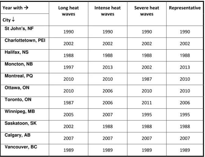
Table 6 lists the extreme years for selected Canadian cities as obtained by the proposed method. All the years encompass heat waves with duration of at least two days, except for the mild weathers of Halifax (NS) and St. John’s (NF) with heat waves of one day duration.
Table 6. Years with extreme heat waves for selected Canadian cities
Year with Long heatwaves Intense heat waves Severe heat waves Representative City St John's, NF 1990 1990 1990 1990 Charlottetown, PEI 2002 2002 2002 2002 Halifax, NS 1988 1988 1988 1988 Moncton, NB 1997 2013 2002 2013 Montreal, PQ 2010 2010 1987 2010 Ottawa, ON 2010 2006 2010 2010 Toronto, ON 1987 2006 2011 2006 Winnipeg, MB 2005 2007 1995 1995 Saskatoon, SK 2002 1988 1988 1988 Calgary, AB 2007 2007 2007 2007 Vancouver, BC 1989 1989 1989 1989
23 6. EFFECTS OF BUILDINGS ON RSWY
Generation of RSWY as presented in Section 5 is based solely on the outdoor weather conditions and are intended to be used in free running buildings where the indoor conditions are direct consequences of the outdoor conditions. It is, however, well known that building constructions and operation, internal heat gains and moisture generation, and occupant behavior may alter the indoor conditions and
therefore extreme indoor overheating events may not be synchronized with extreme outdoor heat wave events. Furthermore, indoor overheating events may be defined differently than outdoor heat events in terms of threshold temperatures and t-SET for day and night time exposures, and reference activity level and clothing insulation of building occupants. In this regard, the outdoor- based RSWY may or may not result in extreme indoor heat events, which are necessary to evaluate the risk of space overheating in applicable standards. One can distinguish three possibilities for outdoor-indoor heat event
synchronisation: (1) extreme outdoor heat events result in extreme indoor overheating events. This fulfils the intent of using the RSWY for building simulation. (2) Extreme outdoor heat events result in less extreme indoor overheating events and therefore RSWY are not suitable to conduct building simulation for overheating risk analysis; and (3) a combination of (1) and (2) where some types but not all of extreme outdoor heat events result in extreme indoor overheating events. This case seems more likely to happen, particularly in passive buildings that optimise the use of solar heat gains in winter and summer and natural ventilation. This case justifies the use of up to three RSWY to account for all types of extreme heat wave events as explained in Section 5.
To answer the aforementioned inquiries, a building archetype model is created for a typical single detached house for the Ottawa (Ontario) location. The house consists of four thermal zones: basement, first floor, second floor, and attic with a foot print area of 80 m2. Windows are distributed uniformly
over the four walls of the first and second floors with a window to wall area ratio of 0.15. Typical constructions for the year 1980 are assigned to the house envelopes with thermal resistances of R11 (h⋅°F⋅ft2)/BTU) for walls and R20 for the attic floor. An average air leakage rate of 6.86 air changes per
hour (ACH) at 50 Pa is taken from a measurement database of old houses for the location under consideration. Typical internal heat gains for people, lighting, equipment and service hot water are taken from the National Building Code of Canada (NRC, 2015).
To be able to study natural ventilation, the whole house air leakage rate is converted to an air flow network assuming a uniform distribution of air leakage over the exterior house envelopes (including the attic floor). The attic space is ventilated using four intentional openings with a total opening area of 1/150 of the attic floor surface area (NRC, 2015). The windows are double glazing and may be opened on demand or covered by interior horizontal Venetian blinds or exterior perforated screen shading with an openness factor of 5%. The house is assumed not air-conditioned for the entire summer period from May to September.
Five configurations of window and shading operation are considered for the simulation study: (1) Windows are closed with closed internal blinds (slats are vertical) for the summer period. This
represents the worst case scenario for space overheating for which solar heat gains are maximum. (2) Windows are open with open internal blinds (slats are horizontal); Windows are opened by 25% if the indoor temperature is higher than 26°C and the outdoor temperature. (3) Windows are open with closed internal blinds. (4) Windows are closed with permanently closed exterior shadings. Solar heat gains are minimized for this case. And (5) windows are open with closed external shadings.