HAL Id: ensl-00565293
https://hal-ens-lyon.archives-ouvertes.fr/ensl-00565293v2
Preprint submitted on 15 Feb 2011
HAL is a multi-disciplinary open access
archive for the deposit and dissemination of sci-entific research documents, whether they are pub-lished or not. The documents may come from
L’archive ouverte pluridisciplinaire HAL, est destinée au dépôt et à la diffusion de documents scientifiques de niveau recherche, publiés ou non, émanant des établissements d’enseignement et de
Trend Filtering via Empirical Mode Decompositions
Azadeh Moghtaderi, Patrick Flandrin, Pierre Borgnat
To cite this version:
Azadeh Moghtaderi, Patrick Flandrin, Pierre Borgnat. Trend Filtering via Empirical Mode Decom-positions. 2011. �ensl-00565293v2�
Trend Filtering via Empirical Mode Decompositions
Azadeh Moghtaderia,b,∗, Patrick Flandrinb, Pierre Borgnatb a
Department of Mathematics and Statistics, Queen’s University Kingston, Ontario, Canada K7L 3N6
b´
Ecole Normale Sup´erieure de Lyon, Laboratoire de Physique 46 all´ee d’Italie 69364 Lyon CEDEX 07, France
Abstract
The present work is concerned with the problem of extracting low-frequency trend from a given time series. To solve this problem, the authors develop a nonparametric technique called empirical mode decomposition (EMD) trend filtering. A key assumption is that the trend is representable as the sum of intrinsic mode functions produced by the EMD. Based on an empirical analy-sis of the EMD, the authors propose an automatic procedure for selecting the requisite intrinsic mode functions. To illustrate the effectiveness of the tech-nique, the authors apply it to simulated time series containing different types of trend, as well as real-world data collected from an environmental study (atmospheric carbon dioxide levels at Mauna Loa Observatory) and from a
large-scale bicycle rental service (rental numbers of Grand Lyon V´elo’v). Keywords: Empirical mode decomposition, trend filtering, adaptive data analysis, monthly mean carbon dioxide cycle, seasonality
1. Introduction
Many real-world time series exhibit a “composite” behavior, in the sense that such a time series can be decomposed into a superposition of two “com-ponents.” Typically one of these components can be classified as “trend,”
✩This document is a collaborative effort. ∗Corresponding author
Email addresses: [email protected](Azadeh Moghtaderi),
[email protected](Patrick Flandrin), [email protected] (Pierre Borgnat)
while the other component is classified as “fluctuation.” (Note that the word “residual” is sometimes used instead of “fluctuation.” In this paper, however,
the term residual will be used in the context of empirical mode decompo-sition; see Section 2.) The problem of effecting such a decomposition, and classifying the resulting components as trend or fluctuation, is called the trend filtering problem (or trend estimation problem). Solving this problem is desirable, since an analysis of the trend component of a time series can often yield valuable information, e.g., for prediction. An obvious initial bar-rier to solving the trend filtering problem is that the terms “decomposition,” “trend,” and “fluctuation” are context-dependent. Indeed, given a time series
generated by a particular physical system, it may be clear (based on physical intuition) how to solve the trend filtering problem. In the absence of physical intuition, it may still be possible to solve the trend filtering problem, pro-vided one makes an ad hoc definition of trend; see (Alexandrov et al., 2008). Such definitions may require extra assumptions concerning the nature of the time series.
A common ad hoc definition of trend is that of a “long-term change in the mean” (Chatfield, 1996; Alexandrov et al., 2008). This definition can lead to approaches which attempt to turn the trend filtering problem into one of regression. For example, it may be reasonable to assume that the time series has a trend component described by a low-degree polynomial. The coefficients of this polynomial can then be estimated by a standard polynomial regression; we again refer to (Alexandrov et al., 2008) for a more comprehensive discussion. Other approaches exist which do not impose such a strict model on the trend. For instance, nonparametric trend filtering assumes that the fluctuation possesses generic stationarity properties, and that the trend can be found by an ad hoc smoothing operation applied to the entire time series, e.g., using the Henderson filter (Henderson, 1916) or the Hodrick–Prescott filter (Hodrick and Prescott, 1997). Yet another possibility is to interpret the trend estimation problem in the frequency-domain sense— for instance, one can assume the trend is represented by a particular set of low-frequency (possibly polynomials or unit root) oscillations. This turns the trend filtering problem into a bona fide filtering problem. Viewed in this way, it may be profitable to use Wiener–Kolmogorov filtering (Pollock, 2006) to solve the trend filtering problem. Finally, it is worthwhile to mention that generalized “trend cycles,” defined as a “short-term trend [that] generally includes cyclical fluctuations,” have also been studied (Alexandrov et al., 2008). Deciding if a trend cycle should be considered as trend (e.g., in any of
the above senses) depends on the application and of course the observation scale.
In this paper, we introduce a novel approach to solving the trend filtering problem. We call this approach empirical mode decomposition trend filtering. It is philosophically similar to the “low-frequency approach” described in the preceding paragraph. Indeed, empirical mode decomposition trend filtering is based on the following definition: Trend is that component of a time series which is “slowly varying” in the sense that it is represented by the “slow-est” intrinsic mode functions produced by the empirical mode decomposition (EMD). Recall (Huang et al., 1998) that the EMD is an algorithm which
de-composes a time series into a finite additive superposition of “intrinsic mode functions,” or IMFs. The IMFs are computed in an iterative fashion—each iteration produces an IMF which is “rapidly varying” relative to the residual time series. Thus our decomposition into components is effected by the EMD. The remaining question is “Which of the IMFs produced by the EMD should be deemed the slowest?” It is precisely this question which is addressed by EMD trend filtering. In particular, we attempt to answer this question by ex-amining certain properties of the IMFs’ energies and zero crossing numbers; these properties were first reported in (Flandrin et al., 2004b; Rilling et al., 2005). We give evidence which supports the fact that certain changes in these properties characterize the tipping point between trend and fluctuation.
It must be mentioned that the use of the EMD to solve the trend filtering problem has already been proposed in the literature. However, such work has either relied on an a priori model for the fluctuation (Flandrin et al., 2004a), or has considered the trend as being the final residual time series produced by the EMD (Wu et al., 2007). In a sense, using the EMD to solve the trend filtering problem shares common features with singular-spectrum anal-ysis applied to the same problem (Vautard and Ghil, 1989; Ghil and Vautard, 1992; Vautard et al., 1991). This is because the SSA also effects a decomposi-tion into oscillatory components. Like the EMD-based method proposed by Wu et al. (2007), a possible approach to solving the trend estimation prob-lem using SSA is to identify the trend as the lowest-frequency oscillatory component. Other possibilities are to look for oscillatory components with prescribed smoothness or monotonicity properties; see (Alexandrov et al., 2008).
The rest of the paper is organized as follows. In Section 2, we briefly review some background material concerning the EMD. In Section 3 we state what trend means in the context of this paper. In Section 4, we describe the
details of EMD trend filtering. The performance of EMD trend filtering is demonstrated in Sections 5, 6 and 7 through analyses of simulated and real-world time series. The concluding remarks are made in Section 8. Finally, the extension of the EMD trend filtering method to multiplicative models is provided in the Appendix.
2. The Empirical Mode Decomposition
The empirical mode decomposition (EMD) is an algorithm which decom-poses a time series into a finite additive superposition of oscillatory compo-nents, each of which is called an intrinsic mode function (IMF); see (Huang et al., 1998). The EMD does not rely on any technical assumptions concern-ing the nature of the time series; note that this includes modellconcern-ing assump-tions. The basic idea is that IMFs are computed subject to two requirements: First, the number of local extrema and number of zero crossings of each IMF vary by at most one. Second, the mean of the upper and lower envelopes of each IMF should be identically equal to zero, where the envelopes are com-puted by means of a fixed interpolation scheme. (In the numerical results presented in this paper, we have confined ourselves to the use of cubic spline interpolation.) The IMFs are computed by means of an iterative scheme. This scheme however depends on a stopping criterion which guarantees that the requirements above are satisfied within a given tolerance while at the same time each extracted IMF is meaningful in both its amplitude and fre-quency modulations; we again refer to (Huang et al., 1998) for details.
To make this intuitive description more precise, let X = {Xt}t≥0 be a
(real, discrete-time, stochastic) process, and let X = (X0, X1, . . . , XN−1) be
a realization of X. (These assumptions illustrate a notational convention that is used throughout the rest of the paper, namely that time series of length N are written in bold typeface and are regarded as elements of the Euclidean space RN.) As an initialization step, set i = 1 and ρ0 = X . The
EMD computes the IMFs of X using the following algorithm. (1) Identify the local maxima and local minima of ρi−1.
(2) Together with the chosen interpolation scheme, use the maxima and minima from step (1) to compute the upper and lower envelopes of ρi−1.
(3) Determine the local trend, denoted Qi, as the mean of the upper and lower envelopes from step (2).
(5) If h is not an IMF, in the sense that it does not satisfy the two require-ments described in the beginning of this section, then increment i and go to step (1) with ρi−1 = h. (Huang et al. (1998) call this the sifting
process; it is this process which depends on the stopping criterion.) (6) If h is an IMF, in the sense that it satisfies the two requirements described
at the beginning of this section, then the ith intrinsic mode function of X is Mi = h, and the ith residual is ρi = X − Mi
. Increment i, then go to step (1).
The algorithm halts when the ith residual has no further oscillations, in the sense that it has no local maxima or local minima. We denote by I the largest index for which Mi is defined. Then
X =
I
X
i=1
Mi+ ρI. (1)
In this decomposition, M1 through MI can be thought of as containing a “spectrum” of local oscillations in X , with the shortest-period (highest frequency) oscillations represented in M1 and the longest-period (lowest frequency) oscillations represented in MI. The computational complexity of the algorithm depends on X , the chosen interpolation scheme, and the stopping criterion. However, the algorithm usually halts in a reasonably small number of steps. For example, it is known (Flandrin et al., 2004a) that if X is a broadband process (a broadband process includes a relatively wide range (or band) of frequencies), then the decomposition produced by the EMD has an almost dyadic filter-bank structure, typically with I ≈ log2N .
Moreover, it is known that the sifting process typically halts after some tens of iterations (Huang et al., 1998).
3. Trend in EMD
As discussed in Section 1, the term “trend” is meaningless and has to be made more precise in order to be useful. In this section we state what we mean by trend in this paper and in the context of EMD trend filtering. To begin with, let us introduce some notation.
Let Y = (Y0, Y1, . . . , YN−1) be a realization of a process Y = {Yt}t≥0,
and let C = (C0, C1, . . . , CN−1) ∈ Rn be a trend component. Assume also
C we may form two new time series: The first is Y + C, the additive mix of Y and C; the second is CY, the multiplicative mix of Y and C. (Here the multiplication is being performed componentwise.) In either case, we say that Y is fluctuation of the mix. Now let X be the additive or multiplicative mix of Y and C. The question we wish to answer is: “Solely given X as data, under what conditions should it be possible to accurately estimate C from X ?” To do so, we must constrain the trend and fluctuation of the mix in some fashion. We take the following pragmatic approach that is based on properties of EMD.
Recall that in EMD, the successive IMFs are oscillations going from high frequency to low frequency, and that this property is valid locally in time (there is not necessarily a global separation of spectrum of successive IMFs) (Huang et al., 1998). A loose “definition” of a trend in this paper is that C is locally slowly varying as compared to Y. Hence, a pragmatic way of satisfying this is that the trend should be obtained as the sum of the last few IMFs and the residual extracted from X .
Let us now turn the attention to some properties of fluctuation of the mix which can also define (in contrast) the trend. First, and in agreement with Flandrin et al. (2004b) and Wu and Huang (2004), the mean frequency of the successive IMFs of broadband processes decrease, similarly to constant-Q filter-banks, with a factor near 2. This will be the first criterion studied in Section 4.1 by estimating the mean frequency from the number of zero crossings of IMFs. Second, the finding of Rilling et al. (2005) is that the “energy” of the IMFs of many broadband processes decreases as the index of the IMFs increases. This has been first reported and demonstrated in Rilling et al. (2005) for fractional Gaussian noise (fGn) processes (Embrechts and Maejima, 2002) which are convenient models for generic broadband processes. We will provide more discussion in Section 4.2 for the validity of these char-acteristics. An explicit assumption in our work is that the fluctuation Y contaminating the trend C have such energy profile. This does not exclude situations with a substantial energy increase downwards low frequencies, as is the case for fGns with Hurst exponent H > 1/2. Indeed the decreasing energy condition does not apply directly to the broadband processes, but to their IMFs. In practice, given the previously mentioned dyadic structure for the IMF spectra, processes Y with power spectra diverging as f−α at the
zero frequency are admissible provided that α < 1.
In the presence of a trend, the prescription used in this paper is that the IMF index which shows a rupture in the two properties described above
separates the trend from the fluctuation. It follows from this prescription that a trend in the present work is neither restricted to be monotonic nor to be some polynomial functions. The trend in this work can however contain oscillations while in Wu et al. (2007) only the residual of EMD was deemed a trend, hence constraining it to have no oscillations at all.
In the following two sections, we will describe in details the properties discussed above and their abilities in separating trend and fluctuation. 4. EMD Trend Filtering
Let X be the additive mix of Y and C, where these entities are given as in the previous section. As described there, our goal is to accurately estimate C from X . This section is devoted to describing EMD trend filtering which can be used to obtain such an estimate.
The following notation and terminology will be employed throughout this section. Let Mi be the IMFs of X , where 1 ≤ i ≤ I, and let i∗ be such that
Ci∗ =
I
X
i=i∗
Mi+ ρI (2)
is the best approximation to C in the Euclidean metric. We call i∗ the best
index and Ci∗ the best approximation of C. Estimating C is equivalent to estimating the best index. If bi∗ is an estimate of i∗, then we denote by bCi∗ the corresponding estimate of C.
EMD trend filtering, described over the course of the next three subsec-tions, actually consists of three approaches to estimating i∗. These are called,
respectively, the ratio, energy, and energy-ratio approaches.
The extension of the trend filtering method to multiplicative mixes in-cluding all simulations can be found in the Appendix.
4.1. Ratio approach
In this subsection we describe the first approach to estimate i∗, which is
based on an empirical property of the zero crossing numbers of IMFs. Let us first establish some additional notation. For a given time series, the zero crossing number of its ith IMF is denoted by Zi, and let us define
Ri = Zi−1/Zi for i ≥ 2. (This is well-defined since Zi ≥ 1; see Section 2.)
Of course, Ri depends fundamentally on the given time series; since the
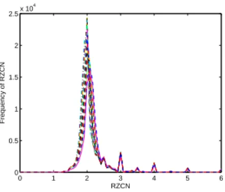
0 1 2 3 4 5 6 0 0.5 1 1.5 2 2.5x 10 4 RZCN Frequency of RZCN
Figure 1: Empirical distribution of the elements of ~R for broadband data: Com-puted for 10000 realizations of 20 broadband processes in the collection. Each line of different type and color associates with a broadband process in the collection.
We call Ri the ith ratio of the zero crossing numbers (ith RZCN). It has been
observed by Flandrin et al. (2004b) and Wu and Huang (2004) that if the time series under study is a realization of a generic broadband process, the approximation Ri ≈ 2 holds.
Let us first support this observation. We considered 20 broadband pro-cesses of the following types: 17 fGn propro-cesses with H = 0.1, 0.15, 0.2, . . . , 0.9, two stationary AR(2) processes, and a nonstationary AR(2) process with time-dependent coefficients. For each process in the collection, we simu-lated B = 10000 realizations of length N = 2000, then computed the IMFs of each realization along with their zero crossing numbers. Denoting the ith RZCN of its bth realization by Ri,b, where 2 ≤ i ≤ Ib, and setting
~
Rb = (R2,b R3,b · · · RIb
,b), we then computed the empirical distribution of
the elements of ~R = ( ~R1 R~2 · · · ~RB). Fig. 1 displays this empirical
distri-bution, and supports the contention that Ri ≈ 2. In fact, this distribution is
approximately Gaussian with mean 2. Furthermore, it is evident from Fig. 1 that apart from the expected peak at 2, we also observe several smaller but visible peaks at higher values. These peaks appear to be due to the presence of high-order IMFs; indeed, these slowly oscillating modes have small zero crossing numbers. Because RZCNs are calculated as the ratio of two integers, if the numerator is a small number, then the distribution of the elements of
~
R will have peaks at integer or rational values such as 2, 5/2, 3, 4/3, etc. Hence, RZCNs with integer or rational values for small denominators have slightly higher expected probabilities than neighbouring values.
Generically, the approximation Ri ≈ 2 fails for i near the best index i
0 1 2 3 4 5 6 0 0.2 0.4 0.6 0.8 1 1.2 1.4 1.6 1.8 2x 10 4 RZCN Frequency of RZCN 0 1 2 3 4 5 6 0 0.2 0.4 0.6 0.8 1 1.2 1.4 1.6 1.8 2x 10 4 RZCN Frequency of RZCN
Figure 2: Empirical distribution of the elements of ~R for additive mixes: Left: Computed for additive mixes obtained by adding C3 from Fig. 5 and realizations of broadband processes in the collection. Right: Computed for detrended additive mixes.
This observation is supported by the following data. For each broadband process in the collection and using its realizations, we constructed 10000 additive mixes, using C3 (displayed in Fig. 5) as a trend. We then computed the IMFs of each mix along with their RZCNs and set ~Rb and ~R as described
earlier. The left-hand plot in Fig. 2 displays the empirical distribution of the elements of ~R for additive mixes, and supports the contention that Ri ≈ 2 fails. In fact this empirical distribution is non-Gaussian as its side
peaks grows taller in comparison with the distribution shown in Fig. 1. The problem however is that it is not yet clear whether Ri ≈ 2 fails around i
∗.
To clarify this, we proceeded with further simulations. For each broadband process in the collection, we used the IMFs obtained for each mix and used the knowledge of C3 to evaluate the best index i
∗ (see Section 5 for details.)
For each mix, we then computed the best approximation of the fluctuation by eliminating those IMFs whose indices are greater than or equal to i∗ (we
call this detrending the mix.) We set ~Rb and ~R for the remaining IMFs and
computed the empirical distribution of the elements of ~R. This distribution, shown in the right-hand plot in Fig. 2, is Gaussian with mean 2 as was the case in Fig. 1. We therefore conclude that Ri ≈ 2 fails around i
∗.
Based on what we described above, we propose to estimate i∗ by choosing
bi∗ to be the smallest index i for which Ri is “significantly different from 2”.
We refer to this as the ratio approach. The results of our simulations for broadband processes suggest that in order to conclude whether or not Ri is
“significantly different from 2”, a common threshold test can be used. For 0 ≤ p ≤ 100, we therefore compute p% and (100 − p)% significance level of
the empirical distribution shown in Fig. 1 as the left threshold and the right threshold respectively. At the end, any RZCN outside of the appropriate right and left thresholds is considered significantly different from 2.
A weakness of the ratio approach is that, since selection of the left and right thresholds is based on empirical results, it is always possible that for a given p, the smallest i for which Ri appears significantly different from 2 is
a false detection. In Section 5, we will discuss how to select an optimum p. 4.2. Energy approach
In this subsection we describe the second approach to estimate i∗, which
is based on an empirical property of the so-called “energy” of the IMFs. To describe this property, we need to establish some additional notation. Let {Zt}t≥0 be an arbitrary process. For a given time series which is a
realization of {Zt}, we define the energy of its ith IMF, denoted Gi, by
Gi , N−1X t=0 |Mi t| 2, 1 ≤ i ≤ I.
Assume now that we have B different time series obtained from {Zt}. Given
the bth time series, 1 ≤ b ≤ B, if Gi,b denotes the energy of its ith IMF, the
averaged energy of its ith IMF is defined by Gi , 1 B
PB
b=1G
i,b.
It is shown in Rilling et al. (2005) that if the time series under study are realizations of a generic broadband process, then Gi is a decreasing sequence
in i. This results were obtained by studying fGn processes. This observation is also supported by the following data. Recall the broadband processes and their realizations from Section 4.1. We computed the IMFs of each realization along with Gi,b and Gi. Fig. 3 displays log
2Gi for 20 broadband processes
in the collection. The result of this simulation supports the idea that Gi is a
decreasing sequence in i when computed for broadband data.
Our key observation is that, generically, Gi increases for i near the best
index i∗. This observation is supported by the following data. Recall the
additive mixes obtained in Section 4.1. We computed the IMFs of each mix along with Gi,b and for each broadband process in the collection, we
computed Gi. The left-hand plot in Fig. 4 displays log
2Gi computed for
additive mixes. For each broadband process in the collection, we observe that Gi increases at some i but we cannot yet determine whether or not it
has occurred around i∗. To clarify this, we detrended each mix as described
1 2 3 4 5 6 7 8 −24 −22 −20 −18 −16 −14 −12 i lo g2 G i Figure 3: log2Gi
: Computed for 10000 realizations of 20 broadband processes in the collection. 1 2 3 4 5 6 7 8 −4 −3 −2 −1 0 1 2 3 4 5 6 i lo g2 G i 1 1.5 2 2.5 3 3.5 4 4.5 5 −4 −3 −2 −1 0 1 2 3 i lo g2 G i Figure 4: log2Gi
: Left: Computed for additive mixes. Right: Computed for detrended additive mixes and displayed only up to i = 5.
broadband process in the collection, we then computed Gi and observed that
Gi increases at the best index i
∗. The right-hand plot in Fig. 4 displays
log2Gi computed for detrended additive mixes only up to i = 5. This is
because for some examples, i∗ > 5 but for the majority i∗ = 5.
Based on the above discussion, identifying the smallest index i ≥ 2 such that Gi > Gi−1 evaluates bi
∗. This approach is called the energy approach.
As for the ratio approach, one could think of looking for significant in-creases which would be based on some statistical information about the dis-persion of energy of each IMF. This viewpoint has been considered first for white Gaussian noise in Huang et al. (2003) and further generalized in Flan-drin and Gon¸calves (2004) and FlanFlan-drin et al. (2004a), even in a detrending perspective. The limitation however is that the associated confidence inter-vals depend strongly on some prior knowledge about the spectra of broadband
processes. This is the main reason that we do not follow such direction, as we are interested in a procedure which is not model-dependent.
A limitation with the energy approach is that one is often given a single time series to use for trend estimation. Computation of energy based on only one time series may cause an increase in Gi when i 6= i
∗.
4.3. Energy-ratio approach
To overcome limitations of the previous approaches, we introduce the last and most important approach to estimate i∗. As described, the energy and
ratio approaches are confronted with possible false detections of the smallest index which does not associate with the trend. Since the criteria proposed by the energy and ratio approaches to evaluate bi∗ are independent, the number
of false detections can be reduced by combining these two approaches. To be more precise, for each 2 ≤ i ≤ I, we compute each index i such that Gi > Gi−1. For a fixed p, we also evaluate every index i where Ri is
significantly different from 2. We then evaluate bi∗ to be the smallest common
index in both approaches. This approach is called the energy-ratio approach. 5. Performance Evaluation of the EMD Trend Filtering;
Evalua-tion of an optimum p
We follow two main goals in this section. The first goal is to evaluate the overall performance of the EMD trend filtering. The second goal is to empirically evaluate an optimum p which can improve the performance of the energy-ratio approach in comparison with the energy and ratio approaches. In order to do so, we use 10 simulated examples including 6 additive and 4 multiplicative mixes such that
Xk = Ck+ Yk, 1 ≤ k ≤ 3 CkYk, 4 ≤ k ≤ 6 (Ck−3− 1) + Yk−3, k = 7 Ck−3+ Yk−3, 8 ≤ k ≤ 9 (Ck−9+ 1)Yk−9, k = 10. (3)
In order to construct the above mixes, we use the following. Let Yk = {Yk
t }t≥0, 1 ≤ k ≤ 6, be 6 generic broadband processes such
that for 1 ≤ k ≤ 2, we have Y1 t = 0.8Y 1 t−1− 0.4Y 1 t−2+ ζt, and Yt2 = 0.2Y 2 t−1+ 0.5Y 2 t−2+ ξt,
500 1000 1500 2000 −0.5 0 0.5 t C 1 500 1000 1500 2000 −0.4 −0.2 0 0.2 0.4 t C 2 500 1000 1500 2000 −0.4 −0.2 0 0.2 0.4 t C 3 500 1000 1500 2000 0.5 1 1.5 t C 4 500 1000 1500 2000 1 1.2 1.4 1.6 1.8 2 t C 5 500 1000 1500 2000 0.5 1 1.5 2 2.5 t C 6
Figure 5: Trends used in simulated examples: Ck for 1 ≤ k ≤ 6.
where {ζt} and {ξt} are two independent white noise processes with variance
104, and for 3 ≤ k ≤ 6, we have 4 fGn processes with Hurst exponents 0.7,
0.5, 0.15, and 0.75 respectively. Let Yk = (Yk
0, Y1k, . . . , YNk−1) be a realization
of Yk. Now, let us assume that Ck = (Ck
0, C1k, . . . , CNk−1), 1 ≤ k ≤ 6, are 6
trends where for 1 ≤ k ≤ 4, we have 4 randomly constructed trends using peacewise linear and cubic spline techniques and for 5 ≤ k ≤ 6, we have
C5 t = 2 − e −(t−1000)2 2×4002 , and C6 t = 1.5 + cos(2πfst), fs= 0.002.
Fig. 5 displays Ck for 1 ≤ k ≤ 6 when N = 2000.
For each k, we created B = 10000 realizations of length N = 2000 of Yk
and constructed the mixes for each realization following Eq. (3). We denote the bth realization of the kth example by bk. In order to achieve the goals
described earlier in this section, we started with the following computations. We applied EMD to Xbk
(or log |Xbk
| for multiplicative mixes) in order to extract its IMFs. Denote I, Mi, and ρI by Ibk, Mibk, and ρIbk respectively.
For each i† ∈ {1, 2, . . . , Ibk}, we computed Cbk i† = Ibk X i=i† Mibk + ρIbk , (4)
and the Euclidean distance (ED) between Ck and Cbk
i†, denoted E
bk
i†. The best index i∗ is that i† which results in minimum Eb
k i†, denoted E bk i∗. Clearly, C bk i∗
is the best approximation of Ck. Let Ybk i∗ = X bk − Cbk i∗. Here Y bk
i∗ is the best approximation of the fluc-tuation Ybk
. We computed the Euclidean norm (EN) of Ybk
i∗ and Y bk and denoted them by EYbk i∗ and E Ybk respectively.
We then estimated Ck using three different trend filtering methods. The methods we used are the Hodrick–Prescott (HP) filter (Hodrick and Prescott, 1997), the singular-spectrum analysis (SSA) (Vautard et al., 1991) and the EMD trend filtering using ratio, energy and energy-ratio approaches. We de-noted the trend estimates obtained above by bCbmk where the letter m indicates the type of trend filtering. For simplicity, we selected m to be r, g, and gr to refer to the ratio, energy, and energy-ratio approaches respectively. Since the ratio and energy-ratio approaches are dependent on p, we denoted the estimates for these methods by bCbmk,p. After all, we computed the ED between Ck and each trend estimate and denoted them by Ebk
m (or Eb k,p
m .)
For each k, we then averaged all the ENs and EDs computed above over B realizations and denoted them by Ekm (or E
k,p
m ). In this paper, in order to
obtain Ekhp, we used two free parameters of 105 and 5 × 10⁵, for Ek
ssa, we used
the window lengths of 100 and 200, and for Ek,pr and E k,p
gr , we used 27 fixed
p where 0 ≤ p ≤ 45. Tables 1, 2, 3, and 4 report all the averaged EDs and ENs computed using these parameters.
To evaluate the performance of the EMD trend filtering which was the first goal in this section, we make two attempts. The first attempt is to compare the best approximation of Ck obtained from the EMD trend filtering with
estimates obtained from the HP filter and the SSA. In order to do so, for each k, we compared the reported EDs from the second column of Table 1 with those from the third to sixth columns. Since these EDs are comparable, we conclude that the EMD trend filtering performs similarly to the HP filter and the SSA. Note that since both HP filter and the SSA are dependent on free parameters, the quality of their performance can vary in comparison
k Eki∗ E k hp E k hp E k ssa E k ssa E Yk i∗ E Yk 1 0.822 0.840 0.697 0.818 0.627 5.475 5.493 2 0.887 0.930 0.785 0.920 0.729 2.854 2.922 3 0.642 0.655 0.581 0.652 0.542 2.334 2.398 4 4.808 6.014 4.898 3.924 3.070 49.73 49.63 5 4.803 6.396 5.212 4.144 2.863 49.75 49.65 6 8.513 7.315 6.123 6.265 13.75 49.45 49.61 7 0.752 0.898 0.733 0.871 0.624 7.392 7.400 8 0.631 0.393 0.286 1.651 0.211 17.32 17.31 9 4.594 4.314 3.850 4.273 3.715 12.47 13.18 10 6.369 7.028 5.732 3.924 3.070 49.84 49.66
Table 1: Performance evaluation of the EMD trend filtering: For 1 ≤ k ≤ 10, the second to sixth columns report the average over B of the EDs between Ckand respectively
Cbk
i∗, C
bk
hpwith free parameter 10
5, Cbk
hpwith free parameter 5×10
5, Cbk
ssawith window length
100, and finally Cbk
ssa with window length 200. The last two columns are the average over
B of the ENs of Ybk i∗ and Y
bk
respectively.
with the EMD trend filtering. This is clear from the reported EDs in Table 1. The second but also necessary attempt we make is to compare the fluctuation of each mix with the best approximation of the fluctuation. This is done by comparing the averaged ENs reported in the last two columns of Table 1. The fact that these two columns are comparable is an indication that the EMD trend filtering is a well-performed method in estimating the trend.
Recall the second goal in this section which is to empirically evaluate an optimum p which makes the energy-ratio approach to perform better than the energy and ratio approaches. We should note that by using the term optimum here, we really mean within the given examples.
In order to obtain such p, we used the averaged EDs reported in Tables 2, 3 and 4. Comparing the values reported in Tables 2 and 3 shows that for ma-jority of p and k, the averaged EDs associated with the energy-ratio approach are smaller than those for the ratio approach. This means that the energy-ratio approach performs better than the energy-ratio approach regardless of p. As a result, selection of p should only depend on how the energy-ratio approach compares with the energy approach. We therefore compare the averaged EDs reported in Table 3 with those reported in Table 4. For each k, we select the smallest p in Table 3 such that Ek,pgr < Ekg and denote it by pk
1. We display
Ek,p k 1
gr in bold in Table 3 and we have pk1 ∈ {11, 5, 10, 1, 3, 11, 16, 1, 13, 9}.
For each k, we observe that for p > pk
1, E
k,p
p E1,pr E 2,p r E 3,p r E 4,p r E 5,p r E 6,p r E 7,p r E 8,p r E 9,p r E 10,p r 1 5.346 5.819 3.441 5.421 6.350 21.62 1.524 0.655 21.43 9.033 3 2.987 3.400 1.807 5.457 5.877 17.44 1.092 0.663 10.86 8.262 5 1.709 1.618 0.917 6.037 6.115 13.20 1.020 0.863 6.927 7.972 7 1.694 1.601 0.916 7.206 7.185 11.72 1.083 1.237 6.847 8.607 8 1.474 1.341 0.838 8.150 8.031 12.31 1.109 1.514 6.558 9.297 9 1.379 1.137 0.770 9.142 8.805 12.29 1.137 1.792 5.977 9.913 10 1.366 1.101 0.759 10.18 9.822 12.76 1.191 2.101 5.752 10.73 11 1.336 1.065 0.750 10.94 10.63 12.99 1.253 2.419 5.550 11.50 12 1.371 1.068 0.760 11.88 11.54 13.73 1.335 2.766 5.506 12.37 13 1.412 1.067 0.770 12.88 12.59 14.45 1.404 3.122 5.456 13.28 14 1.453 1.078 0.782 13.84 13.62 15.23 1.491 3.482 5.463 14.16 15 1.513 1.091 0.797 14.72 14.58 15.94 1.577 3.815 5.465 14.95 16 1.574 1.112 0.814 15.44 15.35 16.54 1.671 9.125 5.508 15.61 17 1.639 1.156 0.837 16.37 16.32 17.35 1.772 4.438 5.559 16.63 18 1.706 1.211 0.858 17.24 17.14 18.08 1.884 4.739 5.629 17.43 19 1.772 1.277 0.880 18.10 18.02 18.94 1.986 5.019 5.720 18.26 20 1.856 1.379 0.912 18.74 18.75 19.65 2.097 5.314 5.832 18.98 22 2.011 1.580 0.983 20.31 20.43 21.25 2.319 5.861 6.135 20.72 24 2.174 1.763 1.059 21.91 22.08 22.97 2.503 6.264 6.535 22.49 26 2.375 1.943 1.156 23.48 23.67 31.54 2.695 6.599 7.083 24.26 28 2.597 2.076 1.258 24.98 25.33 26.15 2.907 6.931 7.639 25.85 30 2.812 2.178 1.350 26.50 26.97 27.76 3.111 7.195 8.149 27.58 32 3.012 2.246 1.436 27.90 28.47 29.30 3.317 7.422 8.594 29.15 34 3.201 2.295 1.511 29.11 29.75 30.62 3.518 7.643 8.965 30.50 35 3.300 2.315 1.546 29.71 30.46 31.37 3.624 7.736 9.158 31.27 40 3.694 2.384 1.695 32.73 33.70 34.41 4.145 8.220 9.892 34.54 45 3.979 2.426 1.794 34.23 35.19 35.81 4.573 8.564 10.34 36.21 Table 2: Averaged EDs for ratio approach: For each k and for 27 selected fixed 1 ≤ p ≤ 45, this table reports the average over B of the EDs between Ck and bCbrk,p.
p E1,pgr E 2,p gr E 3,p gr E 4,p gr E 5,p gr E 6,p gr E 7,p gr E 8,p gr E 9,p gr E 10,p gr 1 3.377 4.346 2.500 5.429 6.359 21.59 1.222 0.654 21.42 9.101 3 2.275 3.174 1.729 5.300 5.729 17.44 1.086 0.633 10.89 8.353 5 1.483 1.584 0.921 5.204 5.229 12.99 0.993 0.633 6.930 7.636 7 1.482 1.582 0.920 5.231 5.246 10.89 0.992 0.633∗ 6.846 7.423 8 1.328 1.355 0.832 5.238 5.252 10.89 0.963 0.634 6.528 7.429 9 1.209 1.137 0.751 5.202∗ 5.103∗ 10.16 0.927 0.634 5.897 7.178 10 1.141 1.092 0.724 5.228 5.133 9.909 0.912 0.635 5.621 7.162 11 1.071 1.047 0.702 5.250 5.173 9.511 0.893 0.635 5.370 7.132 12 1.045 1.037 0.697 5.266 5.191 9.444 0.890 0.636 5.265 7.146 13 1.032 1.024 0.691 5.288 5.229 9.330 0.875 0.636 5.158 7.078∗ 14 1.007 1.024 0.686 5.322 5.270 9.236 0.875 0.637 5.088 7.088 15 0.976 1.020∗ 0.681 5.348 5.300 9.172 0.871 0.638 5.008 7.097 16 0.955 1.026 0.680 5.369 5.317 9.054 0.857 0.639 4.962 7.099 17 0.952 1.052 0.679 5.398 5.356 9.022 0.856 0.640 4.916 7.109 18 0.925 1.085 0.677 5.414 5.389 8.999 0.853 0.642 4.887 7.096 19 0.916 1.135 0.677∗ 5.433 5.412 8.982 0.847 0.642 4.878 7.120 20 0.909 1.217 0.679 5.447 5.429 8.967 0.846 0.643 4.866 7.123 22 0.906 1.370 0.681 5.491 5.484 8.949 0.842 0.645 4.862∗ 7.141 24 0.899∗ 1.516 0.685 5.523 5.537 8.919 0.835∗ 0.647 4.873 7.170 26 0.904 1.668 0.690 5.550 5.578 9.013∗ 0.836 0.648 4.901 7.211 28 0.920 1.790 0.695 5.584 5.620 8.922 0.838 0.649 4.938 7.244 30 0.933 1.880 0.698 5.616 5.666 8.937 0.839 0.650 4.957 7.281 32 0.948 1.957 0.702 5.632 5.684 8.944 0.839 0.651 4.980 7.302 34 0.963 2.013 0.707 5.661 5.724 8.939 0.839 0.652 5.006 7.341 35 0.974 2.036 0.709 5.672 5.736 8.948 0.840 0.652 5.018 7.348 40 1.009 2.124 0.718 5.715 5.793 8.968 0.834 0.656 5.950 7.385 45 1.039 2.177 0.726 5.779 5.860 8.969 0.835 0.657 5.160 7.389 Table 3: Averaged EDs for energy-ratio approach: For each k and for 27 selected fixed 1 ≤ p ≤ 45, this table reports the average over B of the EDs between Ck and bCbgrk,p. For each k, the bold averaged EDs associate with the smallest p where Ek,pgr <E
k
g and the
averaged EDs marked with ∗ are the minimum EDs. The selection is based on four digit decimal points.
k=1 k=2 k=3 k=4 k=5 k=6 k=7 k=8 k=9 k=10 Ekg 1.072 2.220 0.734 5.813 5.906 9.590 0.863 0.659 5.223 7.419
Table 4: Averaged EDs for energy approach: For each k, this table reports the average over B of the EDs between Ck and bCbk
it reaches its minimum (denoted pk
2 and marked with a star in Table 3) and
increases again but it does not exceed Ekg (at least for maximum p = 45.)
This observation indicates that first of all, an optimum p is not unique as it depends strongly on the type of example. Second, there is a wide range of p values which make the energy-ratio approach to perform better that the energy approach. We therefore select an optimum p, denoted p∗ to be
such that p∗ > maxkpk1 and also p∗ < maxkpk2. We therefore can select any
16 < p∗ < 26. In this paper, we use p∗ = 18.
6. Simulated Examples
In this section, we demonstrate the performance of the energy-ratio ap-proach in estimating i∗ via two simulated examples. The examples we use
here are the additive mix X1 and the multiplicative mix X5 introduced in Section 5 for further analysis.
The notation used in this section is exactly the same as in Section 5 except that since we only work with one time series of each mix, we replace bkin the
notation with k. For the ratio and energy-ratio approaches, we use p∗ = 18.
6.1. Simulated example 1
Recall Y1 and C1 from Section 5. Let Y1 = {Y1
0, Y11, . . . , YN−11 } be a
realization of Y1. Set the additive mix X1 = Y1 + C1 for N = 2000. We apply EMD to X1 and extract its IMFs and obtain I = 10.
Using the IMFs obtained for X1, we first compute C1
i† for 1 ≤ i† ≤ 10 as in Eq. (4). We then compute the EDs between C1 and C1
i†, denoted E 1
i†,
and the EDs between X1 and C1i†, denoted E
Y1
i† . These are reported in the first two rows of Table 5. Based on these reported values, we can see that since i† = 8 results in minimum E1i†, we conclude that i∗ = 8. An additional support for this selection is that EY1
8 is the closest value to the EN of Y 1
which is 5.493. We now want to compare the performance of the ratio, energy and energy-ratio approaches in estimating i∗.
Looking at the energy of the IMFs of X1, we observe that the IMF indices
for which Gi > Gi−1 are i = {6, 8, 9, 10}. Based on the energy approach, we
evaluate bi∗ = 6 which is the smallest observed index in this case. Looking at
the RZCN of each IMF on the other hand, we observe that the IMF indices for which Ri is significantly different from 2 are i = {4, 5, 7, 8, 9, 10}. Based
i† 1 2 3 4 5 6 7 8 9 10 11 E1 i† 5.49 4.38 3.21 2.19 1.57 1.2 0.69 0.63 3.80 9.75 -EY1 i† 2.1e-15 3.32 4.64 5.17 5.32 5.38 5.48 5.50 6.61 11.2 -E5 i† 47.4 36.6 27.9 19.7 14.2 10.4 8.25 5.05 3.68 2.49 10.4 EY5 i† 7.5e-14 34.8 40.3 43.9 45.5 46.4 46.9 47.2 47.2 47.2 48.7
Table 5: Search for i∗ in examples 1 and 2: The first two rows are associated with
X1, where 1 ≤ i† ≤ 10. The last two rows are associated with X5, where 1 ≤ i† ≤ 11.
1 2 3 4 5 6 7 8 9 10 −5 0 5 10 i log 2 G i 1 2 3 4 5 6 7 8 9 10 0.5 1 1.5 2 i log 2 R i 0 500 1000 1500 2000 −0.5 0 0.5 t X 1a n d b C 1 gr 0 500 1000 1500 2000 −0.5 0 0.5 t C 1 a n d b C 1 gr
Figure 6: EMD trend filtering for simulated example 1: Top left: The energy approach. The small circles are log2Gi for 1 ≤ i ≤ 10 and the small triangles mark
those indices i ≥ 2 where Gi > Gi−1. Bottom left: The ratio approach. The small
circles are log2Ri for 2 ≤ i ≤ 10 and the small triangles mark those indices i where Ri is
significantly different from 2. The dashed lines are the averaged left and right thresholds of the distribution shown in Fig. 1 when p∗= 18. Top right: X1 vs. bC
1
gr. Bottom right:
C1 (dashed line) vs. bC1gr(solid line).
evaluates bi∗ = 8 as the smallest common IMF index between the energy and
ratio approaches.
It is clear from above that the energy-ratio approach has performed ex-cellently in estimating i∗ by eliminating the false detections in the ratio and
energy approaches. Fig. 6 displays the energy and ratio approaches together with the estimated trend using bi∗.
6.2. Simulated example 2
Recall Y5 and C5 from Section 5. Let Y5 = {Y5
0, Y15, . . . , YN−15 } be a
realization of Y5. Set the multiplicative mix X5 = C5Y5 for N = 2000. We
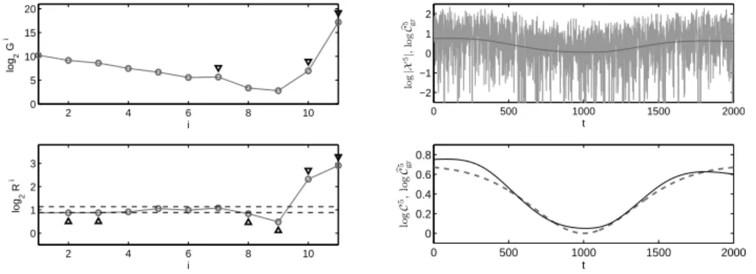
2 4 6 8 10 0 5 10 15 20 i log 2 G i 2 4 6 8 10 0 1 2 3 i log 2 R i 0 500 1000 1500 2000 −2 −1 0 1 2 t lo g |X 5|, lo g b C 5 gr 0 500 1000 1500 2000 0 0.2 0.4 0.6 0.8 t lo g C 5, lo g b C 5 gr
Figure 7: EMD trend filtering for simulated example 2: Top left: The energy approach. Bottom left: The ratio approach. The dashed lines are the averaged left and right thresholds of the distribution shown in the left-hand plot in Fig. 12 when p∗= 18.
Top right: log |X5| vs. log bC5. Bottom right: log C5 (dashed line) vs. log bC5(solid line).
Similarly to the previous example, we use the IMFs obtained for log |X5|
to first compute log C5
i† for 1 ≤ i†≤ 11. We then compute the EDs between log C5 and log C5
i†, denoted E 5
i†, and the EDs between log |X
5| and log C5
i†,
denoted EY5
i† . These are reported in the last two rows of Table 5. Based on these reported values, we can see that since i† = 10 results in minimum E5i†, we conclude that i∗ = 10. An additional support for this selection is that
EY5
10 is the closest to the EN of log |Y
5| which is 47.38. We now compare the
performance of the ratio, energy and energy-ratio approaches in obtaining bi∗.
Looking at the energy of the IMFs of log |X5|, we observe that i =
{7, 10, 11}. Based on the energy approach, we evaluate bi∗ = 7. Looking at the
RZCN of each IMF on the other hand, we observe that i = {2, 3, 8, 9, 10, 11}. Based on the ratio approach, we evaluate bi∗ = 2. Finally, the energy-ratio
approach evaluates bi∗ = 10 as the smallest common IMF index between the
energy and ratio approaches.
It is clear from above that the energy-ratio approach has performed ex-cellently in estimating i∗ by eliminating the false detections in the ratio and
energy approaches. Fig. 7 displays the energy and ratio approaches together with the estimated log-trend using bi∗.
Mar59 Mar69 Mar79 Mar89 Mar99 Mar09 320 330 340 350 360 370 380 390
Months and years
Monthly mean CO
2
Apr Jun Aug Oct Dec Feb −4 −3 −2 −1 0 1 2 3 4 Months of a year
Expected annual cycle(s)
Figure 8: Monthly mean CO2data and the expected annual cycle: Left: Monthly mean CO2 data from March 1958 to March 2010. Right: Yearly cycles of the detrended
data using the expected trend together with their average (dark black line).
7. Real-World Examples
In this section we demonstrate the performance of the energy-ratio ap-proach via two real-world examples. The first example is the monthly mean carbon dioxide (CO2) data from Mauna Loa and the second example is the
Grand Lyon-V´elo’v bicycle rental data from the city of Lyon in France. 7.1. Monthly mean CO2 at Mauna Loa
In this section, we analyze the monthly mean CO2 data collected from
March 1958 to March 2010 and measured at Mauna Loa observatory in Hawaii (Available via FTP:ftp://ftp.cmdl.noaa.gov/ccg/co2/trends /co2 mm mlo.txt. The authors have received permission from Dr. Pieter Tans in order to use this data.) The left-hand plot in Fig. 8 displays the monthly mean CO2 data at Mauna Loa. After removing the averaged
sea-sonal cycle expected in this data, a trend is obtained. This trend is given at the URL together with the data, and it will serve as a reference for a compar-ison with the result from EMD trend filtering. For more information on the known seasonal cycle and trend calculation see the URL provided above. The right-hand plot in Fig. 8 displays the one year cycles of the monthly mean CO2 data after removing the expected trend together with their average. We
call this average the expected annual cycle.
We now use EMD trend filtering for monthly mean CO2 data in order
to estimate its underlying trend. Applying EMD to this data, we obtain I = 3 and following the energy-ratio approach, we evaluate bi∗ = 3. The
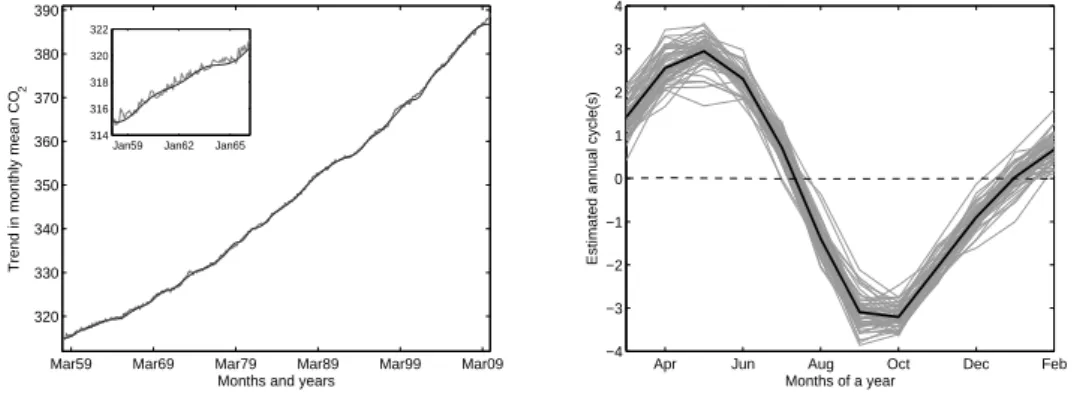
Mar59 Mar69 Mar79 Mar89 Mar99 Mar09 320 330 340 350 360 370 380 390
Months and years
Trend in monthly mean CO
2
Jan59 Jan62 Jan65
314 316 318 320 322
Apr Jun Aug Oct Dec Feb −4 −3 −2 −1 0 1 2 3 4 Months of a year
Estimated annual cycle(s)
Figure 9: Estimated trend and annual cycle for the monthly mean CO2 data: Left: Expected trend together with the estimated trend using EMD trend filtering. Since these two trends look very similar, the smaller plot is made to display only a small portion of these trends. Right: Yearly cycles of the detrended monthly mean CO2data using the
estimated trend together with their average (dark black line). The dashed line displays the difference between the expected and estimated annual cycles.
left-hand plot in Fig. 9 displays the estimated trend plotted together with the expected trend obtained from removing the seasonal cycle. Since these two trends look very similar, the smaller plot is made to display only a small portion of these trends. It is clear that the estimated trend from the EMD trend filtering is only a smoother version of the expected trend.
After subtracting the estimated trend from the data, we divide the de-trended data into one year cycles and then average over all cycles to obtain the estimated annual cycle. The right-hand plot in Fig. 9 displays all the one year cycles of the monthly mean CO2 data after removing the estimated
trend together with the estimated annual cycle. The dashed line in Fig. 9 dis-plays the difference between the expected and estimated annual cycles. This difference confirms the strong similarities between the two annual cycles. 7.2. Grand Lyon-V´elo’v
In this section we analyze the data from V´elo’v, the community shared bicycle program that started in Lyon in May 2005 (for more information, see http://www.velov.grandlyon.com.) The program V´elo’v is a major initiative in public transportation, in which bicycles are proposed to rental by anyone at fully automated stations in many places all over the city, to be returned at any other station. Such a community shared system offers both a new and versatile option of public transportation, and a way to look into the
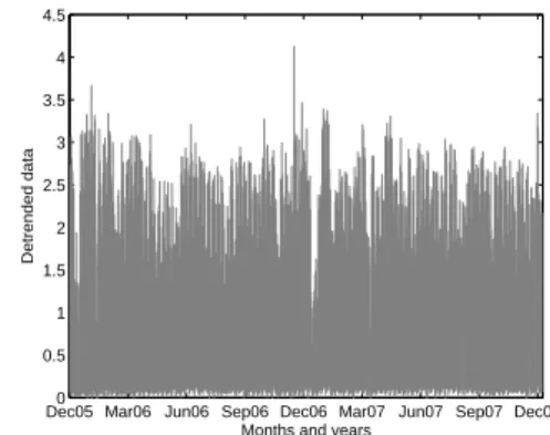
Dec05 Mar06 Jun06 Sep06 Dec06 Mar07 Jun07 Sep07 Dec070 500 1000 1500 2000 2500 3000
Months and years
Raw data and estimated trend
Dec05 Mar06 Jun06 Sep06 Dec06 Mar07 Jun07 Sep07 Dec070 0.5 1 1.5 2 2.5 3 3.5 4 4.5
Months and years
Detrended data
Figure 10: V´elo’v raw and detrended data: Left: The raw V´elo’v data together with the estimated trend using EMD trend filtering. Right: Detrended V´elo’v data.
movements of people across the city. In order to understand the dynamics of this system, a question is to estimate and model the evolution in time of the number of rentals made throughout the city (Borgnat et al., 2009). The left-hand plot in Fig. 10 displays the raw data which is the number of hourly rentals for two years of activity of the V´elo’v system from December 2005 to December 2007. (The authors would like to thank JCDecaux for providing access to this data.)
The number of rentals contains cyclical patterns over the day (e.g., more activities during the day, mainly at specific rush hours, than during the night) and the week (e.g., more activities during week-days than week-ends). It also contains superimposed fluctuations due to external contingencies (e.g., rain or holidays) and a general multiplicative trend over the months (Borgnat et al., 2009). We apply EMD trend filtering to this data in order to estimate the underlying multiplicative trend. We obtain I = 12 and using the energy-ratio approach we evaluate bi∗ = 10 which we use to estimate the trend.
The estimated trend is displayed in the left-hand plot in Fig. 10 where superimposed over the data.
This trend is meaningful for the data, and can be related to, and ex-plained by, two effects: (i) the system was expanded in 2005 and 2006 at the same time it was already in exploitation, hence, there is a long-term increase of the hourly rentals over the two years of data, (ii) because of seasonal ef-fects, the use of V´elo’v is smaller during winter, and also during the main summer holidays; this causes several drops of the trend, during winter and also summer holidays.
Sa Su Mo Tu We Th Fr 0 0.5 1 1.5 2 2.5 3 3.5 4 4.5 Week days
Weekly cycles of detrended data
Figure 11: Weekly detrended V´elo’v data: The weekly cycles of the detrended V´elo’v data and their average (dark black line).
Using the estimated trend, detrended V´elo’v data are obtained by divid-ing the number of hourly locations by the estimated trend. This is displayed in the right-hand plot in Fig. 10. The detrended data is, visually, more stationary than the raw data. This allows a good estimation of the cyclic pattern over the week of the number of hourly rentals. Fig. 11 displays the weekly cycles of the V´elo’v data after removing the estimated trend, and the average over all the weeks.
The estimate of the average usage of the V´elo’v bicycles as a function of time in the week, is meaningful in that it reveals the main features of the V´elo’v activity: during week-days, there are three sharp peaks of rentals in the morning, noon and the end of the afternoon; during the week-ends, there are small peaks at noon, and smooth and large peaks during the afternoon.
Finally, let us note that here the multiplicative trend estimation procedure was applied to a case where the underlying process that the trend multiplies to is not actually a broadband process: it is more specifically a periodic pro-cess (with clear periods of one week and one day) with added fluctuation. Nevertheless, the procedure is able to find the relevant multiplicative trend describing the evolutions at the scale of the seasons, and that is used to de-trend the data. This is believed to be due mostly to the fact that fluctuations have typical periodic scales (one day or one week) which are much smaller than the typical scale of evolution (several months) of the trend, making of this scale separation a prerequisite that might be more important than the existence of a broadband spectrum in a stricter sense.
8. Conclusion
An automated method has been proposed to filter the trend in a time series, whose principle is to extract the lowest frequency intrinsic mode func-tions (IMFs) via empirical mode decomposition (EMD). The core of the method is to decide which IMFs belong to the trend, on the rationale that a trend causes both a departure of the ratio of zero crossing numbers from 2, and an increase of the energy contained in the low-frequency IMFs, as com-pared to the expected behavior of broadband processes. Combining both criteria, the procedure was shown to work well on several examples with additive or multiplicative trends. We emphasize that the approach is fully data-driven (as is EMD) and, besides the parameters of the decomposition itself, the EMD trend filtering method has only one free parameter which is the level of significance p.
Many numerical examples were reported to illustrate the robustness of the EMD trend filtering and its potential interests have been further illustrated on two real-world examples: the CO2 data which displays an additive trend,
and the V´elo’v data which shows a multiplicative trend. In both cases, filter-ing of the trends allows us to propose an estimation of the cycle inside the data (annual cycle for the CO2 data, weekly and daily cycles for the V´elo’v
data) that compares favorably to existing methods both for the extracted trends and estimated cycles. A strength of the method is that it works, even if the fluctuations above the trend do not follow exactly a priori behaviors for the fluctuation that where used to design empirically the test (displaying for instance oscillatory behaviors more than the assumed broadband behav-ior.) This is related to its character as a fully data-driven and model-free approach.
A perspective of this work would be to go beyond trend-filtering and use the same type of approach to group together IMFs obtained by EMD in several signals describing a trend, then the major cycles, and finally the rapid fluctuation. This would be an interesting asset for the model-free decomposition of processes.
9. Acknowledgement
The authors would like to thank the anonymous reviewers and Associate Editor for their helpful comments and suggestions. Most of the work re-ported here was completed during the postdoctoral stay of Azadeh
Mogh-taderi at ENS Lyon, which was supported by ANR Grant ANR-07-BLAN-0191-01 StaRAC.
References
Alexandrov, T., Bianconcini, S., Dagum, E. B., Maass, P., McElroy, T., March 2008. A review of some modern approaches to the problem of trend extraction. Research Report Series, Statistics #2008-3, Statistical Research Division, U.S. Census Bureau, Washington. To appear in Econo-metric Reviews.
Borgnat, P., Abry, P., Flandrin, P., Rouquier, J.-B., 2009. Studying Lyon’s V´elo’v: A statistical cyclic model. In: Proceedings of ECCS’09 (European Conference of Complex Systems). Warwick, United Kingdom.
Chatfield, C., 1996. The analysis of time series: An introduction. Chapman and Hall/CRC.
Embrechts, P., Maejima, M., 2002. Selfsimilar Processes. Princeton Univer-sity Press, Princeton, NJ.
Flandrin, P., Gon¸calves, P., 2004. Empirical mode decompositions as data-driven wavelet-like expansions. International Journal of Wavelets, Multires-olution and Information Processing 2 (4), 477–496.
Flandrin, P., Gon¸calves, P., Rilling, G., 2004a. Detrending and denoising with empirical mode decompositions. In: Proceedings of EUSIPCO-04. Vienna, Austria, pp. 1581–1584.
Flandrin, P., Rilling, G., Gon¸calves, P., 2004b. Empirical mode decomposi-tion as a filter bank. IEEE Signal Processing Letters 11 (2), 112–114. Ghil, M., Vautard, R., 1992. Interdecadal oscillations and the warming trend
in global temperature time series. Nature 58, 95–126.
Henderson, R., 1916. Note on graduation by adjusted average. Transactions on the Actuarial Society of America 17, 43–48.
Hodrick, R. J., Prescott, E. C., 1997. Postwar U.S. business cycles: An empirical investigation. Journal of Money, Credit, and Banking 29 (1), 1–16.
Huang, N. E., Shen, Z., Long, S. R., Wu, M. L., Shih, H. H., Zheng, Q., Yen, N. C., Tung, C. C., Liu, H. H., 1998. The empirical mode decomposition and Hilbert spectrum for nonlinear and non-stationary time series analysis. Proceedings of the Royal Society of London A: Mathematical, Physical and Engineering Sciences 454, 903–995.
Huang, N. E., Wu, M.-L., Long, S., Shen, S., Qu, W., Gloersen, P., Fan, K., 2003. A confidence limit for the empirical mode decomposition and Hilbert spectral analysis. Proceedings of the Royal Society of London A 459 (2037), 2317–2345.
Pollock, D. S. G., 2006. Wiener–Kolmogorov filtering frequency-selective fil-tering and polynomial regression. Econometric Theory 23, 71–83.
Rilling, G., Flandrin, P., Gon¸calves, P., 2005. Empirical mode decomposition, fractional Gaussian noise, and Hurst exponent estimation. IEEE Interna-tional Conference on Acoustics, Speech, and Signal Processing, 489–492. Vautard, R., Ghil, M., 1989. Singular-spectrum analysis in nonlinear
dynam-ics with applications to paleoclimatic time series. Physica D 35, 395–424. Vautard, R., Yiou, P., Ghil, M., 1991. Singular-spectrum analysis: A toolkit
for short, noisy chaotic signals. Physica D 350, 324–327.
Wu, Z., Huang, N. E., 2004. A study of the characteristics of white noise using the empirical mode decomposition method. Proceedings of the Royal Society of London A 460, 1597–1611.
Wu, Z., Huang, N. E., Long, S., Peng, C.-K., 2007. On the trend, detrending, and variability of nonlinear and nonstationary time series. Proceedings of the National Academy of Sciences 4 (38), 14889–14894.
Appendix. EMD Trend Filtering for Multiplicative Mixes
If the mix is multiplicative and the elements of C are positive, then the situation reduces to the additive case. Indeed, one can take logarithms to obtain log |X | = log C +log |Y|, where the logarithm and absolute value func-tions are being applied elementwise. The main question arising is whether the properties regarding the energy and ratio of the zero crossing numbers
0 1 2 3 4 5 6 0 0.2 0.4 0.6 0.8 1 1.2 1.4 1.6 1.8 2x 10 4 RZCN Frequency of RZCN 1 2 3 4 5 6 7 8 3 4 5 6 7 8 9 10 11 i lo g2 G i
Figure 12: Empirical distribution of the elements of ~R and log2Gi
for log-transformed broadband data: Computed for 10000 log-transformed realizations of 20 broadband processes in the collection. Each line of different type and color associates with a broadband process in the collection.
of the IMFs in the additive case are still valid for the multiplicative ones. To validate such properties, we proceeded by using the same simulations which were proposed in Sections 4.1 and 4.2 for broadband data and additive mixes.
We first recall 20 broadband processes and their realizations from Section 4.1. We computed the IMFs of the log-transform of the absolute value of each realization along with their zero crossing numbers and energy. We set
~
Rb and Gi,b and then ~R and Gi as described in Sections 4.1 and 4.2. The
left-hand plot in Fig. 12 displays the empirical distribution of the elements of ~R and it supports the contention that Ri ≈ 2. In fact, this distribution
is approximately Gaussian with mean 2. The right-hand plot of Fig. 12 on the other hand displays log2Gi and supports the contention that energy is a
decreasing sequence in i for log-transformed broadband data.
Similar to the additive mixes, the approximation Ri ≈ 2 expects to fail
and also Gi expects to increase for i near the best index i
∗. These
observa-tions are supported by the following data. For each broadband process in the collection and using its realizations, we constructed 10000 multiplicative mixes, using 1 + C3 (displayed in Fig. 5) as a trend. We then computed the IMFs of the log-transformed absolute value of each mix and set ~Rb, Gi,b,
~
R, and Gi as described earlier. The top left-hand plot in Fig. 13 displays
the empirical distribution of the elements of ~R and the top right-hand plot displays log2Gi both for log-transformed multiplicative mixes. Similarly to
Sections 4.1 and 4.2, for each broadband process in the collection, we used the IMFs obtained for each log-transformed mix and used the knowledge of
0 1 2 3 4 5 6 0 0.2 0.4 0.6 0.8 1 1.2 1.4 1.6 1.8 2x 10 4 RZCN Frequency of RZCN 1 2 3 4 5 6 7 8 9 4 6 8 10 12 14 16 i lo g2 G i 0 1 2 3 4 5 6 0 0.2 0.4 0.6 0.8 1 1.2 1.4 1.6 1.8 2x 10 4 RZCN Frequency of RZCN 1 2 3 4 5 6 7 4 5 6 7 8 9 10 11 i lo g2 G i
Figure 13: Empirical distribution of the elements of ~R and log2Gi
for log-transformed multiplicative mixes: Left: Computed for log-transformed multiplicative mixes obtained by multiplying 1 + C3from Fig. 5 and realizations of broadband processes in the collection. Right: Computed for detrended log-transformed multiplicative mixes.
log C3 to evaluate the best index i
∗. We then used i∗ to detrend each
log-transformed mix and recomputed ~Rb, Gi,b, ~R, and Gifor the remaining IMFs.
The bottom left-hand plot in Fig. 13 displays the empirical distribution of the elements of ~R and the bottom right-hand plot displays log2Gi both for
detrended log-transformed multiplicative mixes. The comparison between the left-hand and the right-hand plots in Fig. 13 indicates that Ri ≈ 2 fails
and Gi increases both at the best index i
∗.
These simulations altogether validate the fact that, after log-transformation, multiplicative mixes have properties similar to the additive mixes. Hence, the energy-ratio approach is expected to operate in a similar way to estimate the log-transformed trend, with the exception that the left and right thresholds used for the ratio approach are different. The appropriate left and right thresholds are now p% and (100 − p)% significance level of the empirical distribution shown in the left-hand plot in Fig. 12.