Line graphs, link partitions, and overlapping communities

RESEARCH OUTPUTS / RÉSULTATS DE RECHERCHE

Author(s) - Auteur(s) :

Publication date - Date de publication :

Permanent link - Permalien :

Rights / License - Licence de droit d’auteur :

Bibliothèque Universitaire Moretus Plantin

Institutional Repository - Research Portal

Dépôt Institutionnel - Portail de la Recherche

researchportal.unamur.be

University of Namur

Line graphs, link partitions, and overlapping communities

Evans, T.S.; Lambiotte, R.

Published in:

Physical Review E - Statistical, Nonlinear, and Soft Matter Physics

DOI:

10.1103/PhysRevE.80.016105 Publication date:

2009

Document Version

Publisher's PDF, also known as Version of record

Link to publication

Citation for pulished version (HARVARD):

Evans, TS & Lambiotte, R 2009, 'Line graphs, link partitions, and overlapping communities', Physical Review E

-Statistical, Nonlinear, and Soft Matter Physics, vol. 80, no. 1. https://doi.org/10.1103/PhysRevE.80.016105

General rights

Copyright and moral rights for the publications made accessible in the public portal are retained by the authors and/or other copyright owners and it is a condition of accessing publications that users recognise and abide by the legal requirements associated with these rights. • Users may download and print one copy of any publication from the public portal for the purpose of private study or research. • You may not further distribute the material or use it for any profit-making activity or commercial gain

• You may freely distribute the URL identifying the publication in the public portal ?

Take down policy

If you believe that this document breaches copyright please contact us providing details, and we will remove access to the work immediately and investigate your claim.

Line graphs, link partitions, and overlapping communities

T. S. Evans1,2and R. Lambiotte1 1

Institute for Mathematical Sciences, Imperial College London, SW7 2PG London, United Kingdom

2

Theoretical Physics, Imperial College London, SW7 2AZ London, United Kingdom 共Received 12 March 2009; published 9 July 2009兲

In this paper, we use a partition of the links of a network in order to uncover its community structure. This approach allows for communities to overlap at nodes so that nodes may be in more than one community. We do this by making a node partition of the line graph of the original network. In this way we show that any algorithm that produces a partition of nodes can be used to produce a partition of links. We discuss the role of the degree heterogeneity and propose a weighted version of the line graph in order to account for this. DOI:10.1103/PhysRevE.80.016105 PACS number共s兲: 89.75.⫺k, 02.50.Le, 05.50.⫹q, 75.10.Hk

I. INTRODUCTION

Finding hidden patterns or regularities in data sets is a universal problem that has a long tradition in many disci-plines from computer science 关1兴 to social sciences 关2兴. For

example, when the data set can be represented as a graph, i.e., a set of elements and their pairwise relationships, one often searches for tightly knit sets of nodes usually called communities or modules. The identification of such commu-nities is particularly crucial for large network data sets that require new mathematical tools and computer algorithms for their interpretation. Most community detection methods find a partition of the set of nodes where most of the links are concentrated within the communities关3,4兴. Here the

commu-nities are the elements of the partition and so each node is in one and only one community.

A popular class of algorithms seeks to optimize the modu-larity Q of the partition of the nodes of a graph G关5–9兴. The

simplest definition of modularity for an undirected graph, i.e., the adjacency matrix A is symmetric, is关10兴

Q共A兲 = 1

WC

兺

兺

冋

kikj

W

册

where W =兺i,jAij and ki=兺jAij is the degree of node i. The

indices i and j run over the N nodes of the graph G. The index C runs over the communities of the partitionP. Modu-larity counts the number of links between all pairs of nodes belonging to the same community and compares it to the expected number of such links for an equivalent random graph in which the degree of all nodes has been left un-changed. By construction 兩Q兩ⱕ1 with larger Q indicating that more links remain within communities then would be expected in the random model. Uncovering a node partition that optimizes modularity is therefore likely to produce use-ful communities.

This node partitioning approach has, however, the draw-back that nodes are attributed to only one community, which may be an undesirable constraint for networks made of highly overlapping communities. This would be the case, for instance, for social networks, where individuals typically be-long to different communities, each characterized by a cer-tain type of relation, e.g., friendship, family, or work. In scientific collaboration networks共for example 关11兴兲, authors

may belong to different research groups characterized by

dif-ferent research interests. Such intercommunity individuals are often of great interest as they broker the flow of informa-tion between otherwise disconnected contacts, thereby con-necting people with different ideas, interests, and perspec-tives 关12,13兴.

Only a few alternative approaches have been proposed in order to uncover overlapping communities of nodes, for ex-ample关14–16兴. Our suggestion is to define communities as a

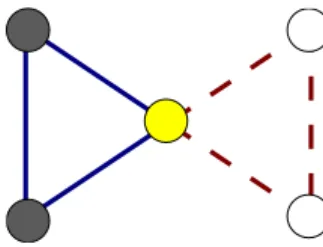
partition of the links rather than of the set of nodes. A node may then have links belonging to several communities and in this it belongs to several communities. The central node in a bow tie graph is a simple example; see Fig. 1. This link partition approach should be especially efficient in situations when the nodes of a network are connected by different types of links, i.e., in situations where the nodes are heterogeneous while the links are very homogeneous. In the case of the social network mentioned above, this would occur when the friendship network and work network of individuals only have a very small overlap.

This paper is organized as follows. In Sec.II, we review a definition of modularity that uses the statistical properties of a dynamical process taking place on the nodes of a graph. In Sec. III, we propose three dynamical processes taking place on the links of the graph and derive their corresponding modularities, now defined for a partition of the links of a network. To do so, we make connections to the concept of a line graph and with the projection of bipartite networks. In Sec. IV, we optimize the three modularities for some ex-amples and interpret our results. In Sec.Vwe conclude and propose ways to improve our method.

FIG. 1. 共Color online兲 By partitioning the links of a network into communities, one may uncover overlapping communities for the nodes by noting that a node belongs to the communities of its links. In this toy example, a meaningful partition consists in divid-ing the links into two groups共straight blue lines and the dashed red lines兲. In that case, the central node belongs to the two communities because it is at the interface between these link communities.

II. DYNAMICAL FORMULATION OF MODULARITY To motivate our link partition quality function, let us first consider how to interpret the usual modularity Q关Eq. 共1兲兴 in

terms of a random walker moving on the nodes关17,18兴.

Sup-pose that the density of random walkers on node i at step n is

pi;n and the dynamics is given by

pi;n+1=

兺

Aij

kj

pj;n. 共2兲

From now on, we will only consider networks that are undi-rected共the adjacency matrix is symmetric兲, connected 共there exists a path between all pairs of nodes兲, nonbipartite 共it is not possible to divide the network into two sets of nodes such that there is no link between nodes of the same set兲, and simple 共without self-loops nor multiple links兲. If the first three conditions are respected, it is easy to show关19兴 that the

stationary solution of the dynamics is generically given by

piⴱ= ki/W.

Let us now consider a node partitionP of the network and focus on one community C苸P. If the system is at equilib-rium, it is straightforward to show that the probability a ran-dom walker is in C on two successive time steps is

兺

while the probability of finding two independent walkers at nodes in C are

兺

i,j苸C

kikj

共W兲2. 共4兲

This observation allows us to reinterpret Q as a summation over the communities of the difference of these two prob-abilities. This interpretation suggests natural generalizations of modularity allowing to tune its resolution. Indeed, Q is based on paths of length one but it can readily be generalized to paths of arbitrary length as

R共A,n兲 = 1 WC

兺

兺

冋

册

where Tij= Aij/kj. This quantity is called the stability of

the partition 关17兴. Because kj is an eigenvector of

eigen-value one of T, one can show that the symmetric matrix

X共n兲ij=共Tn兲ijkjcorresponds to a time-dependent graph where

the degree of node i is always equal to ki. Therefore R共A,n兲

can be interpreted as the modularity of X共n兲ij, a matrix that

connects more and more distant nodes of the original adja-cency matrix A as time n grows 关18兴. It can be shown that

optimizing Eq.共5兲 typically leads to partitions made of larger

and larger communities for increasing times and that the op-timal partition when n→⬁ is made of two communities 关17,18兴.

III. LINK PARTITION A. Random walking the links

The above discussion suggests that we should look at a random walker moving on the links of network in order to define the quality of a link partition. Such a walker would therefore be located on the links instead of the nodes at each time n and move between adjacent links, i.e., links having one node in common. In the case of the random walk on the nodes 关Eq. 共2兲兴, a walker at node i follows one of its links

with probability 1/ki, i.e., all links are treated equally.

How-ever, a link between nodes i and j is characterized by two quantities ki and kj, so a random walk on the links is more

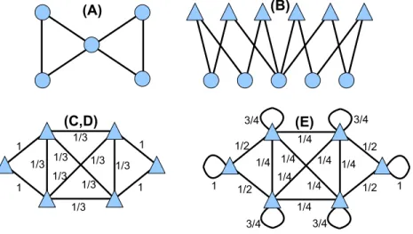
subtle. In the following, we will focus on two different types of dynamical processes that account differently for the de-grees kiand kj共see Fig.2兲.

In the first process, a walker jumps with the same prob-ability 1/共ki+ kj− 2兲 to one of the links leaving i and j. When

ki⫽kj, the walker goes with a different probability through i

or j, and we therefore call this process a “link-link random walk”关see Fig.2共a兲兴.

In the second process, a walker jumps to one of the two nodes to which it is attached, say i, then moves to a link attached to that node共excluding the link it came from兲. Thus it will arrive at a link leaving node i with a probability 1/关2共ki− 1兲兴, and similarly it will arrive at a link attached to

the other node j with probability 1/关2共kj− 1兲兴. We will refer

to this as a “link-node-link random walk” 关see Fig. 2共b兲兴. This process is well defined unless the link is a leaf, namely, one of its extremities has a degree 1, say i. In that case, the walker will jump with a probability 1/共kj− 1兲 to one of the

links leaving j.

These two types of dynamics are different in general ex-cept if the degrees at the extremities i and j of each link are

FIG. 2.共Color online兲 Illustration of the two types of random walk considered in this paper. In both cases, the walkers are situated on the links of a graph, here starting from the central red dashed link. In共a兲 the link-link random walk is shown where the walker jumps 共the green dashed arrows兲 to any of the adjacent links with equal probability. In 共b兲 a link-node-link random walk is illustrated. In this case the walker moves first to a neighboring node with equal probability and then moves on to a new link chosen with equal probability from those new links incident at the node.

T. S. EVANS AND R. LAMBIOTTE PHYSICAL REVIEW E 80, 016105共2009兲

equal. In the case of a connected graph, this condition is equivalent to demanding that the graph is regular, i.e., the degree of all the nodes is a constant. When this condition is not respected, the link-link random walk favors the passage of the walker through the extremity having the largest de-gree. The difference between the two processes will be maxi-mal when the network is strongly disassortative, namely, when links typically relate nodes with very different degrees 关20兴.

B. Projecting the incidence matrix

1. Bipartite structure

In order to study these two types of random walk more carefully, it is useful to represent a network G by its inci-dence matrix B. The elements Bi␣of this N⫻L matrix 共L is

the number of links兲 are equal to 1 if link␣is related to node

i and 0 otherwise. The incidence matrix of G may be seen as

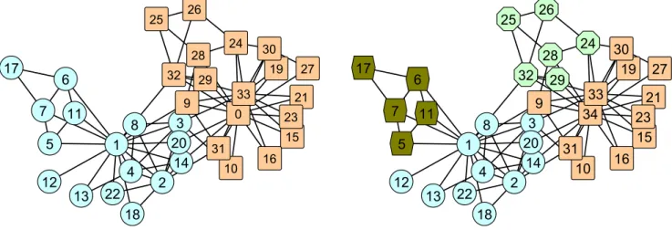
the adjacency matrix of a bipartite network I共G兲 关see Fig.

3共b兲兴, the incidence graph1 of G where the two types of nodes correspond to the nodes and the links of the original graph G. By construction, all the information of the graph is incorporated in B. For instance, the degree kiof a node i and

the number of nodes k_␣attached to a link␣共always equal to 2兲 are given by ki=

兺

兺

The N⫻N adjacency matrix A of the graph G can also be obtained

Aij=

兺

␣ Bi␣Bj␣− ki␦ij. 共7兲

This operation 共7兲 can be interpreted as a projection of the

bipartite incidence graph I共G兲 onto the unipartite network G 关21,22兴. In a similar way, an adjacency matrix for the links

can be obtained by projecting the bipartite network onto its links. In the following, we will focus on two standard types of projection that, as we will show, are directly related to the two random walks introduced above.

2. Line graph

The simplest way to project a bipartite graph consists of taking all the nodes of one type for the nodes of the projected graph. A link is added between two nodes in this projected graph if these two nodes had at least one node of the other type in common in the original bipartite graph. Operation共7兲

is of this type. When applied to the links ␣of the graph G, the second type of vertex in the bipartite incidence graph

I共G兲, it leads to the L⫻L adjacency matrix C whose

ele-ments are

C_␣␤=

兺

i

Bi␣Bi␤共1 −␦␣␤兲. 共8兲

It is easy to verify that this adjacency matrix is symmetric and that its elements are equal to 1 if two links have one node in common, and zero otherwise. It is interesting to note that this adjacency matrix corresponds to another well-known graph, usually called the line graph of G 关23兴 and

denoted by L共G兲 关see Fig. 3共c兲兴. It is a simple graph with L

nodes. By construction, each node i of degree kiof the

origi-nal graph G corresponds to a ki fully connected clique in

L共G兲. Thus it has 兺iki共ki− 1兲/2=O共具k2典N兲 links. Line graphs

have been studied extensively and among their well-known properties, Whitney’s uniqueness theorem states that the structure of G can be recovered completely from its line 1_{An incidence graph is usually defined in terms of the incidence of}

a set of lines with a set of points in a Euclidean space of finite dimension. Here we have a special case where we embed our graph G in some Euclidean space of no particular interest and each link of G is a line that always intersects with exactly two points.

FIG. 3.共Color online兲 The information of the bow tie graph in 共a兲, as encoded by the adjacency matrix A of Eq. 共7兲, has other equivalent graph representations. In共b兲 the incidence matrix 关B of Eq. 共7兲兴 of the bow tie is shown as a bipartite network, the incidence graph I共G兲. The line graph of the bow tie, L共G兲, is the unweighted version of the graph labeled 共c兲,共d兲 with adjacency matrix C of Eq. 共8兲. The weighted version in diagram共c兲,共d兲 has an adjacency matrix D of Eq. 共11兲. The weighted line graph with self-loops labeled 共e兲 has an adjacency matrix E of Eq.共14兲. Circles represent entities that correspond to nodes of the original graph, while triangles come from links in the original graph.

graph L共G兲 for any graph other than a triangle or a star network of four nodes关24兴. This result implies that

project-ing the incidence matrix onto L共G兲 does not lead to any loss of information from the network structure. This is a remark-able result that is not generally true when projecting generic bipartite networks.

It is now straightforward to express the dynamics of link-link random walk 关Fig.2共a兲兴 in terms of the projected adja-cency matrix C,

p_␣;n+1=

兺

␤ C_␣␤

k_␤ p␤;n. 共9兲

Now p_␣;nis the density of random walkers on link␣at step

n, k_␣=兺_␤C_␣␤=共ki+ kj− 2兲 and where i and j are the

extremi-ties of␣. This dynamical process therefore only depends on the sum of the degrees i and j. The stationary solution is found to be p_␣ⴱ= k_␣/W, where W=兺_␣␤C_␣␤. When G is simple, then W =兺i共ki− 1兲ki. By reapplying the steps

de-scribed in关18兴, it is now straightforward to derive a quality

function for the link partitionP of the graph G,

Q共C兲 = 1

WC

兺

兺

冋

C_␣␤−k␣k␤

W

册

This is just the usual modularity 共1兲 for a graph with

adja-cency matrix C.

As we noted, a single node i in G leads to a connected clique of ki共ki− 1兲/2 links in the line graph L共G兲. This seems

to suggest that the line graph L共G兲 gives too much promi-nence to the high degree nodes of the original graph G. Our response is to define a weighted line graph whose links are scaled by a factor of O共1/ki兲.

3. Weighted line graph

In order to derive the quality of a link partition associated to the link-node-link random walk, it is useful to project the incidence matrix in a different way and to define another graph D共G兲 with a symmetric adjacency matrix given by

D_␣␤=

兺

i,ki⬎1

Bi␣Bi␤

ki− 1

共1 −␦␣␤兲. 共11兲

This weighted line graph has the intuitive property that the degree k_␣=兺_␤D_␣␤of a link␣is equal to 2共a link always has two extremities兲 unless␣is a leaf in G共then k_␣= 1 except for one trivial case兲. For example this weighted line graph of the bow tie network is shown in Fig.3共d兲. Only if G is regular will this weighted line graph D共G兲 be equivalent 共up to an overall scale兲 to the original unweighted line graph L共G兲.

This construction is a well-known method for projecting bipartite networks. For instance in the case of collaboration networks 关11兴 the 共ki− 1兲 normalization is justified by the

desire that two authors should be less connected if they wrote a joint paper with many co-authors than a paper with few authors.

This weighted line graph allows us to write the dynamics of the link-node-link random walk in a natural way

p_␣;n+1=

兺

␤ D_␣␤

k_␤ p␤;n 共12兲

and, by reusing the above arguments to define another qual-ity function for the link partition P of a graph

Q共D兲 = 1

WC

兺

兺

冋

D_␣␤−k␣k␤

W

册

where W =兺_␣␤D_␣␤= 2L − Lleafis twice the number of links L

minus the number of leaves in the original graph G, L_leaf. Again, this is the same functional form as the usual modu-larity, Q共A兲 of Eq. 共1兲, only the adjacency matrix has

changed.

C. Projection of a node random walk

The random walks proposed in the previous sections have been defined on the line graph and therefore consist of walk-ers moving among adjacent links of the original graph G. However, such processes cannot be related to the original random walk共3兲 on the nodes of G, because a walker

mov-ing on links can pass at two subsequent steps through the same node of G while such self-loops are forbidden in Eq. 共3兲. This observation suggests an alternative approach where

the dynamics would be driven by the original random walk 共3兲 but would be projected on the links of the network. To do

so, let us assume that a walker has not moved yet and is located at node i. In that case, it is reasonable to assume that all the neighboring links of i are connected by a weight 1/ki.

The corresponding adjacency matrix E for the links is there-fore given by E_␣␤=

兺

. Unlike our pre-vious line graph constructions, C of Eq. 共8兲 and D of Eq.

共11兲, this weighted line graph E共G兲 has self-loops. It is

illus-trated for the bow tie graph in Fig.3共e兲. All nodes␣in E共G兲 have strength 2,兺_␤E_␣␤= 2, reflecting the fact that the links in the original graph G all have two ends.

E is constructed when a walker is located on a node and

has not moved yet. The motion of the walker according to Eq. 共3兲 generates a new adjacency matrix, E₁, defined as

2

One might also try to argue that since an undirected link is both incoming and outgoing, we might deem it appropriate to allow␣ to ␣ transitions in the link-link walk of Fig. 2共a兲. That is, we could define an unweighted line graph with self-loops with adjacency ma-trix C˜_␣␤=兺iBi␣Bi␤. Since it differs from the standard unweighted line graph L共G兲 only by the addition of a self-loop to every node␣, this can be interpreted within the scheme of关29兴 who add self-loops to control the number and size of communities found.

T. S. EVANS AND R. LAMBIOTTE PHYSICAL REVIEW E 80, 016105共2009兲

E_1;␣␤=

兺

i,ki⬎0

Bi␣AijBi␤

kikj

, 共15兲

where we note that E1= EE− E. The corresponding graph is

still regular with k_␣=兺_␤E_1;␣␤= 2, and it is again weighted with self-loops. The quality function associated with this dy-namics is simply Q共E1兲 = 1 WC

兺

兺

冋

册

This quality function is particularly interesting because it has a simple relationship to the modularity of the original graph, Q共A兲 of Eq. 共1兲. To show this let us assign a weight

V_␣crepresenting the strength of the membership of link␣in community c. Such weights may be defined and constrained in many ways. For instance, in a link partition we have

V_␣cV_␣d=␦cdfor any␣, i.e., every link␣belongs to just one

community. In order to translate V_␣cinto a community struc-ture on the nodes, it is natural to use the incidence matrix B of Eq.共7兲 and to define the rectangular matrix Victhrough

Vic=

兺

␣ Bi␣

ki

V_␣c. 共17兲

If V_␣cis a link partition then the projected node community structure Vic is simply the fraction of links in community c

incident at node i. Also if兺cV␣c= 1 then so is兺cVic= 1.

Now using the definition of the adjacency matrix in Eq. 共7兲, we find that the modularity of the original graph G for

some node community Vicis

Q共E1;兵V␣c其兲 = 1 W

兺

兺

冋

册

兺

兺

冋

册

Thus finding modularity optimal link partitions of the line graph with adjacency matrix E1of Eq.共15兲 is equivalent to

the optimization of the modularity of the original graph but with a different constraint on the node community Vicfrom

that imposed when finding node partitions. IV. EMPIRICAL ANALYSIS

A. Methodology

In the previous sections, we have proposed three quality functions Q共C兲, Q共D兲, and Q共E1兲 for the partition of the

links of a network G. Each represents a different dynamical process and therefore explores the structure of the original graph G in a different way. In order to tune the resolution of the optimal partitions, it is straightforward to define the sta-bilities R共C,n兲, R共D,n兲, and R共E1, n兲 of the three processes

by generalizing the concept of modularity to paths of arbi-trary length 共see Sec. II兲. The optimal partitions of these

quality functions can be found by applying standard modu-larity optimization algorithms to the corresponding line graphs. In this paper, we have used two different algorithms 关7,8兴 and have verified that both algorithms give consistent

results.

As a first check, let us look at the bow tie graph of Fig.1. The optimization of the three quality functions Q共C兲, Q共D兲, and Q共E1兲 lead to the expected partition into two triangles,

with the values Q共C兲=0.1, Q共D兲=0.278, and Q共E1兲=0.167.

In this case, the central node belongs equally to the two link communities, a situation that is a far superior way to split the network than a node partition. The best node partition gives

Q共A兲=0.111 when three nodes in one triangle form one

community and the remaining two nodes form a second com-munity.

In order to compare node partitions and link partitions in the following, we will use the idea of a “boundary link” and a “boundary node.” A boundary link of a node partition is one that connects two nodes from different communities. We will then define a boundary node of a link partition to be a node that is connected to links from more than one link community. Thus the central node of the bow tie graph is a boundary node.

B. Karate club

A less contrived graph is the Karate club of Zachary关2兴,

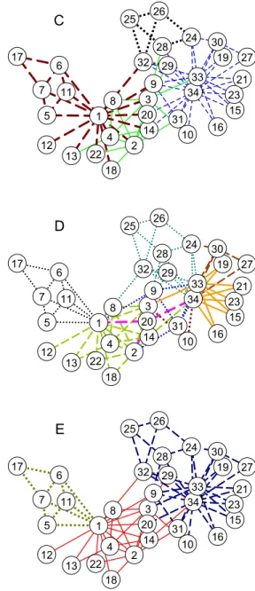
which is made of 34 members. Historically this split into two distinct factions. It is standard to compare the partition pro-duced by a community detection method to the actual split of the club. The node partition having the largest value of modularity Q共A兲=0.420 contains four communities, but the resolution can be lowered by optimizing the stability R共A,n兲 for larger values of n. When n is large enough, the optimal partition is always made of two communities 共see Fig. 4兲,

e.g., R共A,11兲=0.078, which agree with Zachary’s partition into “sink” and “source” communities 关2兴 using the

Ford-Fulkerson binary community algorithm 关25兴.

The link partitions found by optimizing Q共C兲=0.5,

Q共D兲=0.53, and Q共E1兲=0.36 are shown in Fig.5. They are,

respectively, made of four, seven, and three communities. These three partitions are consistent with the historical way split of the network, as the boundary links of the two-way partition of Fig. 4are always connected to a boundary node of a link partition. In general, however, the three opti-mal partitions are as different as their corresponding dynami-cal processes are. The most striking difference is observed around node 1. In the node partition optimizing Q共A兲, this node is connected to several boundary links and connects the community of nodes共5,6,7,11,17兲 to the rest of the network. Such a position is consistent with the link partitions obtained from Q共D兲 and Q共E1兲, but not with the link partition

opti-mizing Q共C兲. In this latter case, one observes that node 1 is rather the focus of one of the link communities on the left-hand side in Fig.5. This difference originates from the high degree of node 1, which implies that a link-link random walk is biased to pass through this node共see Fig.2兲 and therefore

heavily connects its adjacent links. This is a general problem of the unweighted line graph C that gives too much emphasis to high degree nodes共also noted in 关27兴兲 and therefore tends

to produces communities centered around hubs. Such a prob-lem does not take place for the weighted line graphs D and

E₁, and in both these cases node 1 is a boundary node, part of several communities. The main difference between the optimal partitions of Q共D兲 and Q共E1兲 is the number of the

communities in each, as expected because the line graph E₁ connects more distance links of the original graph than D. Let us also note that the optimal partition of Q共E1兲 resembles

very much the one of Q共A兲, as suggested by Eq. 共20兲.

Before concluding, let illustrate how longer random walks can be used to tune the resolution of the link partition. We focus on the weighted line graph D, whose optimal partition into seven communities is difficult to compare against the standard two and four community node partitions of Fig.4. Let us therefore focus on the stability R共D,n兲, which is based on paths of length n of a random walker on D. As expected, larger and larger communities are uncovered when

n is increased and, when n is large enough, we obtain a two

way link partition 共see Fig. 6兲 that shows a perfect match

with the node partition shown in Fig.4.

C. Word associations

As a final example, let us use the University of South Florida Free Association Norms data set 关28兴 to create a

simple network3 in the manner of 关14兴. We obtain a link

partition by optimizing the modularity for the weighted line graph D of Eq. 共11兲 but where the null model term

共k␣k␤兲/W2 has been scaled by a factor of 10.0 in order to

control the resolution 关9兴 and in this case obtain 321

com-munities in the whole network. The corresponding quality function can be seen as a linear approximation of the stabil-ity R共D,n兲 关18兴. It is easier to optimize for large networks.

In Fig. 7 we show part of the network near the word “bright” which is part of 11 communities4. The topology of our communities is much less constrained than those of

k-clique percolation 关14兴, which means we can pick out a

wider range of structures. There are some tight cliquelike subsets, e.g., the names of the planets. At the other extreme the method finds more treelike structures such as the se-quence “lit-on-switch-lever-handle,” which is the backbone of another community linked to bright. On the other hand this flexibility in the structure can produce a confusing pic-ture since many words are members of several communities though mostly having just one or two links per community. For instance for the word “bright,” it is linked to eight of its 11 communities by just one link. However one can exploit this feature to start to define strength of membership in dif-ferent communities. For instance for visualization, we have found it useful to view only those words that have a large number of links within one community, as in Fig.7.

V. DISCUSSION

When describing a network, there seems to be a natural tendency to put the emphasis on its nodes whereas a graph is both a set of nodes and a set of links. It is therefore not surprising that node partitioning has been studied extensively in recent years while link partitioning has been overlooked so far. In this paper, we have shown that the quality of a link

3

We take the sum of the two forward strengths of all pairs of normed word and add a link only if the total is greater than 0.025. We end up with 5018 words connected by 58 536 links and from this a line graph with 1 266 910 links is created.

4

The 11 communities that contain “bright” are well characterized by the following subsets of words: 共“brave,” “bold,” “daring”兲, 共“bright,” “light,” “sunshine”兲, 共“gone,” “fade,” “dim”兲, 共“power,” “electric,” “lightning,” “flash”兲, 共“brain,” “intelligence,” “bril-liant”兲, 共“great,” “wonderful,” “gifted”兲, 共“pen,” “paper,” “high-light”兲, 共“handle,” “lit,” “on,” “switch,” “lever”兲, 共“cloudy,” “gray,” “shiny,” “sunny”兲, 共“space,” “sky,” “moonlight,” “stars”兲, 共“as-sume,” “illusion,” “imagination,” “vivid”兲. However “bright” has 16 of its 29 links in the community containing “sunshine” and “light” with just a single link to eight of its 11 communities. FIG. 4. 共Color online兲 Optimal node partitions for the unweighted Karate club data of Zachary, notation as in 关2兴. On the left is the partition into two communities made by Zachary 关2兴 using the Ford-Fulkerson binary community algorithm 关25兴. It is also produced by optimizing R共A,11兲 of Eq. 共5兲. The right-hand figure shows the node partition with optimal Q共A兲=0.420 关26兴, which contains four communities.

T. S. EVANS AND R. LAMBIOTTE PHYSICAL REVIEW E 80, 016105共2009兲

partition can be evaluated by the modularity of its corre-sponding line graph. We have highlighted that optimizing the modularity of some of our weighted line graphs uncovers meaningful link partitions. Our approach has several advan-tages. A key criticism of the popular node partitioning meth-ods is that a node must be in one single community whereas it is often more appropriate to attribute a node to several different communities. Link partitioning overcomes this limitation in a natural way. Moreover, the equivalence of a link partition of a graph G with the node partitioning of the corresponding line graph L共G兲 means that one can use an existing node partitioning code with only the expense of pro-ducing a line graph transformation and an O共具k2_{典/具k典兲}

in-crease in memory to accommodate the larger line graph.

Even the memory cost can be reduced to be O共1兲 since we have shown our link partitioning is equivalent to a process occurring on the links of the original graph G, so a line graph need not be produced explicitly.

Our method can be seen as a generalization of the popular

k-clique percolation 关14兴, which finds sets of connected k

cliques. By way of comparison we find collections of two cliques, which are more densely connected than expected in an equivalent null model. Thus the link partitioning of our paper can be seen as an extension of two-clique percolation that allows for the uncovering of finer modules, i.e., two-clique percolation trivially uncovers connected components. An interesting generalization would be to apply our approach to the case of triangles, four cliques, etc. To do so, one has to replace the incidence matrix共relating nodes and links兲 by a more general bipartite graph, representing the membership of

FIG. 5. 共Color online兲 The optimal link partitions of 共c兲 Q共C兲, 共d兲 Q共D兲, and 共e兲 Q共E1兲 for the Karate club. They contain four,

seven, and three communities, respectively. The two smallest com-munities in the center of 共d兲 consist of the links: 共a兲 兵共3,10兲, 共10,34兲其, 共b兲 兵共0,20兲, 共1,20兲, 共2,20兲其.

FIG. 6. 共Color online兲 Optimal link partition into two commu-nities of the stability R共D,10兲 of the Karate club.

FIG. 7. 共Color online兲 The simple graph created from the South Florida Free Association Norms data 关28兴, in the manner of 关14兴. The link partition shown is produced by optimizing a modified ver-sion of the modularity Q共D兲 where the null model factor was 10.0⫻共k␣k␤兲/W2_{. This controls the number of communities found}

关9兴. The subgraph shown contains the word “bright” along with nodes that have at least 90% of their links in one of the communi-ties connected to “bright.”

nodes in a clique of interest. Our random walk analysis in terms of this bipartite graph would then proceed in the same fashion and should allow to uncover finer modules than those obtained by k-clique percolation.

All our expressions also hold for the case of weighted networks. Even multiedges can be accommodated if we start from the incidence matrix, B. However the beauty of our approach is that any type of graph analysis, be it community detection or something else, can be applied to a line graph rather than the original graph. In this way, one can view a network from a completely different angle yet use well

established techniques to obtain fresh information about its structure.

ACKNOWLEDGMENTS

R.L. would like to thank M. Barahona and V. Eguiluz for interesting discussions and EPSRC-GB for support. After this work was finished, we received the paper of Ahn et al. 关27兴 who also look at edge partitions but not in terms of

weighted line graphs.

关1兴 M. Fiedler, Czech. Math. J. 25, 619 共1975兲. 关2兴 W. Zachary, J. Anthropol. Res. 33, 452 共1977兲.

关3兴 S. Fortunato and C. Castellano, in Encyclopedia of Complexity and System Science, edited by R. A. Meyers共Springer-Verlag, Berlin, 2009兲.

关4兴 M. A. Porter, J.-P. Onnela, and P. J. Mucha, e-print arXiv:0902.3788.

关5兴 M. E. J. Newman, Phys. Rev. E 69, 066133 共2004兲.

关6兴 R. Guimera, M. Sales-Pardo, and L. A. N. Amaral, Phys. Rev. E 70, 025101共R兲 共2004兲.

关7兴 V. D. Blondel, J.-L. Guillaume, R. Lambiotte, and E. Lefebvre, J. Stat. Mech.共2008兲 P10008.

关8兴 A. Noack and R. Rotta, Lect. Notes Comput. Sci. 5526, 257 共2009兲.

关9兴 J. Reichardt and S. Bornholdt, Phys. Rev. E 74, 016110 共2006兲.

关10兴 M. Girvan and M. E. J. Newman, Proc. Natl. Acad. Sci. U.S.A.

99, 7821共2002兲.

关11兴 M. E. J. Newman, Phys. Rev. E 64, 016131 共2001兲. 关12兴 R. S. Burt, Am. J. Sociol. 110, 349 共2004兲.

关13兴 R. Lambiotte and P. Panzarasa, J. Informetrics 3, 180 共2009兲. 关14兴 G. Palla, I. Derényi, I. Farkas, and T. Vicsek, Nature 共London兲

435, 814共2005兲.

关15兴 V. Nicosia, G. Mangioni, V. Carchiolo, and M. Malgeri, J. Stat. Mech.共2009兲 P03024.

关16兴 A. Lancichinetti, S. Fortunato, and J. Kertész, New J. Phys.

11, 033015共2009兲.

关17兴 J.-C. Delvenne, S. Yaliraki, and M. Barahona, e-print arXiv:0812.1811.

关18兴 R. Lambiotte, J.-C. Delvenne, and M. Barahona, e-print arXiv:0812.1770.

关19兴 F. R. K. Chung, Spectral Graph Theory, CBMS Regional Con-ference Series in Mathematics.

关20兴 M. E. J. Newman, Phys. Rev. Lett. 89, 208701 共2002兲. 关21兴 T. Zhou, J. Ren, M. Medo, and Y.-C. Zhang, Phys. Rev. E 76,

046115共2007兲.

关22兴 R. Lambiotte and M. Ausloos, Phys. Rev. E 72, 066107 共2005兲.

关23兴 V. K. Balakrishnan, Schaum’s Outline of Graph Theory 共Mcgraw-Hill Publishing Company, New York, 1997兲. 关24兴 H. Whitney, Am. J. Math. 54, 150 共1932兲.

关25兴 L. R. Ford and D. R. Fulkerson, Can. J. Math. 8, 399 共1956兲. 关26兴 G. Agarwal and D. Kempe, Eur. Phys. J. B 66, 409 共2008兲. 关27兴 Y.-Y. Ahn, J. P. Bagrow, and S. Lehmann, e-print

arXiv:0903.3178.

关28兴 D. L. Nelson, C. L. McEvoy, and T. A. Schreiber, The Univer-sity of South Florida, word association, rhyme, and word frag-ment norms, http://www.usf.edu/FreeAssociation/

关29兴 A. Arenas, A. Fernandez, and S. Gomez, New J. Phys. 10, 053039共2008兲.

T. S. EVANS AND R. LAMBIOTTE PHYSICAL REVIEW E 80, 016105共2009兲