HAL Id: hal-01792118
https://hal-amu.archives-ouvertes.fr/hal-01792118
Submitted on 15 May 2018
HAL is a multi-disciplinary open access
archive for the deposit and dissemination of
sci-entific research documents, whether they are
pub-lished or not. The documents may come from
teaching and research institutions in France or
abroad, or from public or private research centers.
L’archive ouverte pluridisciplinaire HAL, est
destinée au dépôt et à la diffusion de documents
scientifiques de niveau recherche, publiés ou non,
émanant des établissements d’enseignement et de
recherche français ou étrangers, des laboratoires
publics ou privés.
Weather Routing Optimization: A New Shortest Path
Algorithm
Estelle Chauveau, Philippe Jégou, Nicolas Prcovic
To cite this version:
Estelle Chauveau, Philippe Jégou, Nicolas Prcovic. Weather Routing Optimization: A New Shortest
Path Algorithm. 29th IEEE International Conference on Tools with Artificial Intelligence, ICTAI
2017, Nov 2017, Boston, United States. �hal-01792118�
Weather Routing Optimization:
A New Shortest Path Algorithm
Estelle Chauveau
Atosand
AMU, CNRS, ENSAM LSIS UMR 7296, 13397 Marseille
Email: estelle.chauveau@lsis.org
Philippe J´egou
AMU, CNRS, ENSAM LSIS UMR 7296, 13397 MarseilleEmail: philippe.jegou@lsis.org
Nicolas Prcovic
AMU, CNRS, ENSAM LSIS UMR 7296, 13397 MarseilleEmail: nicolas.prcovic@lsis.org
Abstract—This paper presents an algorithm which solves the
multiobjective shortest path problem in a time-dependent graph, taking advantage of the specificities of the weather routing problem. Multicriteria shortest path problems are widely studied in the literature, as well as monocriteria shortest path problems in time-dependent graphs. Their solving has numerous applications, especially in the transportation field. However, the combination of both these issues is not studied as much as each one separately. In this paper, we study the weather routing problem for cargo ships, which involves optimizing the ship routes following real-time weather information. For this problem, the arc weights on the graph have a low dispersion around their average value. We propose an extension of an algorithm (NAMOA*) taking advantage of this property. We study the validity of this new algorithm and explain why it solves efficiently the weather routing problem. Experiments done using real weather data corroborates the algorithm efficiency.
I. INTRODUCTION
While the Shortest Path Problem in directed graphs is well known to be easy to solve, the Shortest Weight-Constrained Path Problem, which is a simple extension with only one additional criterion, is NP-complete [10]. The bicriteria shortest path problem (associated optimization problem) is NP-hard. Naturally, the difficulty of the problem directly depends on the number of criteria.
A large number of similar problems have been studied in literature, and the most recent algorithms are able to solve large instances in some milliseconds [11], [12], [3]! However, these algorithms are based on methods like contraction hierarchies or overlay graphs which have never been experimented on multiobjective problems in a time dependent graph, but only on problems with a lower complexity. Moreover, these methods are designed for road network specific structures (with large highways linking the main cities). Obviously, this structure cannot be met on ocean roads: even if sea lanes exist between major ports, the space stays continuous, which allows to modify the trajectory slightly so as to benefit from better weather conditions. For this reason, it is not particularly relevant to try them on our problem.
In weather routing optimization, the problem modelling must handle the real time perturbations (traffic disruptions, weather hazards. . . ). This paper deals with the multiobjective shortest path problem in a graph for which arc weights can change
over the time (called ”time-dependent” graph). Among the multiobjective shortest path algorithms, the label setting algorithms turn out to be particularly effective in practice. One of them, the algorithm NAMOA* introduced by Mandow and De La Cruz [21] stands out with the use of a heuristic provided with properties ensuring to find the whole set of optimal paths, while visiting the minimum number of vertices. Thus, we propose here to extend NAMOA* to handle dynamic graphs, that is, valued graphs whose weights on arcs can change during the search. This is motivated by a real world problem: the optimization of cargo ship routes. The considered graph matches an ocean mesh while the modifications of arc weights are justified by the evolution of weather conditions. Solving this problem efficiently has a major environmental concern as sea shipping of goods represents 80% of the worldwide trade in volume [1]. Furthermore, ship owners could substantially reduce their cost as 40% of the operational fees are absorbed by the fuel price during a cargo trip [16]. However, the ship speed reduction leads to a decrease of fuel consumption: the fuel optimization conflicts with the aim to reduce the trip duration. They depend on the weather parameters that change during the time, introducing a dynamic nature to this issue. The goal of this paper is to present an algorithm that takes advantage of the data properties of the problem: arc weights have a low dispersion around their average value. This implies that the optimized roads will be slightly different from the shortest ones (in distance). However, savings due to the reduction of fuel consumption are significant and fret companies are extremely interested in using these algorithms. Furthermore, savings when considering a large fleet can become huge. In this paper, we firstly present a mathematic modeling of the problem and summarize the different relevant prior works (section 2). The new algorithm is detailed in section 3, followed by the experiments (section 4).
II. MULTICRITERIASHORTESTPATHPROBLEM IN A
TIME-DEPENDENT GRAPH
A. Problem Definition
The multiobjective shortest path problem (MSPP, whose first formulation was introduced by Vincke in [25]), is a NP-hard problem [15]. It has not a unique solution, but a set
of solutions that are called the Pareto-optimal paths. In [15], Hansen evidenced a class of graphs for which the number of solutions, i.e. of Pareto-optimal paths, is an exponential function of the number of vertices in the graph. There exists a subclass of MSPP problems for which the arc cost function has features that make the problem tractable. For example, in the bi-objective case, if one cost function is a linear combination of the other one, the problem can easily be reduced to a monocriteria problem. For the problem we study in section IV, the cost functions (e.g. trip duration, fuel consumption) following the weather conditions are complex functions that do not possess such features. The problem we study matches with the MSPP in a graph for which the cost of each arc depends on time. So, algorithms suitable for the standard MSPP are not appropriate. Now we introduce a model to express the multicriteria shortest path problem in a time-dependent graph where time is discretized. ”Time-dependent” means that arc weights are a function of the time. In such a graph, when an arc exists from a vertex i to a vertex j, then the symmetric arc exists and its valuation is not necessarily identical. Consequently, we deal with a directed graph with cycle in which the weighting are positive values (e.g. time, fuel consumption, various risks). The frozen arc model [24] will be used: the arc cost is determined at the arrival time at the tail of the arc and does not change during its traversal.
Input Instance.: Let G = (V, A, T, −→c )be a directed graph where V is a finite set of vertices {i1, i2, . . . in}, A is a set
of arcs, T is a finite set of dates {t0, t1, t2, . . .} representing
the time and −→c is the cost function (A × T → Rk). −→c
ij(t)
represents the approximation of the cost for crossing an arc
(i, j) leaving the vertex i at the date t. More precisely, if
t∈ [ti, ti+1[(with ti, ti+1 ∈ T ) then :
− →cij(t) = ! −→cij(ti)if ti+1t−t−tii < 0.5 − →cij(ti+1)else. −
→cij(t) returns a k-dimension vector, where k is the
number of criteria of the problem. That is −→cij(t) =
([−→cij(t)]1, [−→cij(t)]2, . . . [−→cij(t)]k). All the valuations depend
on the time, and by convention, the first element [−→cij(t)]1 of the vector is the duration (for crossing (i, j)). Let o, d ∈ V be
the origin and the destination vertex, an initial date t0 ∈ T ,
and a maximal date tmax ∈ T . A path (we only consider
elementary paths here) in G from i0 to iq is a sequence of q
arcs < (i0, i1), (i1, i2), . . . , (iq−1, iq) > in which i0, i1, . . . iq
are distinct vertices. Let Pij(t)be the set of paths from i to j so
that the vertex i is left at time t, and that the vertex j is reached at time t" ∈ T . Given a path p
ij(t)∈ Pij(t), with i %= j, we
recursively define the total cost −→C of this path. If pij(t)has
a unique arc (i, j) ∈ A, then −→C (pij(t)) = −→cij(t). Else, the
path pij(t) is compounded by the path pih followed by the
arc (h, j), in which case, −→C (pij(t)) = −→C (pih(t)) + −→chj(t")
with t" = t + [−→C (p
ih(t))]1. And for other components of
the vector, that is ∀l, 1 < l ≤ k, we have [−→C (pij(t))]l =
[−→C (pih(t))]l+ [−→chj(t + [−→C (pih(t))]1)]l. Before defining the
expected solution of the problem, that is optimal paths, we need to recall some definitions about Pareto optimality. Let ≺
be the partial order relation called dominance [20].
Definition 1 (Pareto dominance (1)). In a minimization context,
a cost vector −→c of size k dominates a cost vector −→c " of size
kif: ∀i, 1 ≤ i ≤ k, [−→c ]i≤ [−→c "]i and −→c %= −→c ".
This is denoted −→c ≺ −→c ".
Definition 2 (Pareto dominance (2)). In a minimization context,
a set C of cost vectors of size k dominates a cost vector −→c "
of size k if: ∃−→c ∈ C s.t. −→c ≺ −→c ".
This is denoted C ≺ −→c.
Definition 3 (Pareto-optimality). A vector −→c belonging to a
set C of vectors is pareto optimal inside this set if and only if C ⊀ −→c.
Definition 4 (Optimality principle). The optimality principle in
a graph insures that the subpaths of an optimal path are optimal paths (and this is true for any chosen optimality criteria).
The expected solution of the problem is the subset
P∗
od(t0)∈ Pod(t0)of non dominated paths (in Pareto
mean-ing), with p∗
od(t0) ∈ Pod∗(t0) if and only if: "pod(t0) ∈
Pod(t0) s.t. −→C (pod(t0))≺ −→C (p∗od(t0)).
B. Prior Works
The complexity of the problem is justified by two features: it is multicriteria and time dependent. We can find these two features in other transportation fields (road, railway). This leads to the production of various algorithms which we mention in this section in the following order: (1) multi-objective shortest path problems, (2) monocriteria shortest path problems in a time-dependent graph, and (3) these two issues simultaneously. Note that we consider here exclusively the
admissible algorithms, that is, if a solution exists, the algorithm
guarantees to find it, with Pareto optimality criteria.
1) Multi-objective Shortest Path Problems. Algorithms
solving MSPP generally belong to one of the following three classes: the labelling algorithms, the ranking methods [6], and the parametric approaches [23]. Note that for a deep review of the literature in the multicriteria shortest paths field, the study of Ehrgott and Gandibleux [20] is a reference. Nevertheless, labelling algorithms are the most frequently considered since they usually provide good results, and various evolutions have been proposed over time, like [4], [9] and [2]. More recently (2005) [21] distinguishes itself with the use of a heuristic. This paper presents the algorithm NAMOA*(given in details in section III-B) for which, if the heuristic is consistent (what is equivalent to monotonous), then the algorithm is admissible.
2) Monocriteria Shortest Path Problems in a
Time-Dependent Graph. The monocriteria shortest path prob-lem in a time-dependent graph has been introduced in [7] where the travel durations on arcs are considered as general functions of time, and a discrete time value grid
is used. This paper describes an algorithm based on the Bellman optimality principle (see definition 4).
Later, [8] proposed a method based on the Dijkstra algorithm, claiming that the problem can be solved as efficiently as its static counterpart. Actually, this statement is true only in the case of a FIFO graph
[18], that is for graphs G = (V, A, T, −→c ) such that
∀(i, j) ∈ A, ∀t, t" ∈ T with t < t", we have
t + [−→cij(t)]1 ≤ t" + [−→cij(t")]1. For such graphs, [5] has defined a label-setting algorithm identifying the best paths for all the dates of departure from the root vertex, and [17] mentions an A* based version. Note that in this paper, we consider graphs which are not necessarily FIFO.
3) Multicriteria Shortest Path Problem in a
Time-Dependent Graph. The combination of both issues (mul-ticriteria and time-dependent graph) has been considered for the first time in [19] which relies on the Cooke and Halsey works [7]. They propose two algorithms based on dynamic programming considering FIFO graphs in which the arc cost functions are decreasing. Later [13], such hypothesis were considered for the route computing in urban context. Hamacher et al. works (2006) presented in [14] show that in FIFO graph in which waiting is not authorized in a vertex, Bellman principle of optimality is true only in backward direction, in other words in the case where the algorithm first visit the destination vertex, then its predecessor and so on. Then they suggest a label-setting algorithm. More recently, Veneti [24] studied the time-dependent bi-criteria shortest path problems in non FIFO networks, applied to the sea weather routing, with fixed departure time, no waiting at vertices and a constraint on the total travel time. They proposed a label-setting algorithm based on the Martins one [22], and they compare their results with Hamacher’s results, showing the practical advantages of their algorithm on such instances.
Note that the shortest path in a time-dependent graph requires to study the applicability of the Bellman principle of optimality, that is frequently used in shortest path algorithms (see definition 4) but which is not preserved here:
Theorem 1. [14] In a time-dependent graph, the optimality
principle is not preserved: a Pareto-optimal path is not necessarily compounded of Pareto-optimal subpaths.
III. FROMNAMOA*TONAMOA*-TTOHANDLETIME
A. Choice of extension of NAMOA*
During a computation of shortest paths between two vertices, some vertices don’t need to be visited by the algorithm, since the best complete paths they can belong to are dominated
by already computed solutions (belonging to Pod(t0)). For
example, if we consider a trip from Rio de Janeiro to Cape Town, the partial paths passing through the Pacific Ocean or the Indian Ocean can be quickly filtered by the algorithm, and this, even if the weather conditions in the Atlantic Ocean are
bad. Some admissible algorithms allow to take into account this remark, like NAMOA* (for New Algorithm for Multi-Objective A*) proposed by Mandow and De La Cruz in [21]. This algorithm solves the MSPP for static graphs using an optimistic heuristic. With this heuristic, partial paths are explored in the most relevant order and many useless path explorations can be avoided. Within the scope of sea route optimization, data are structured in this way: arc weights distribution on the different arcs of the graph have a low dispersion (standard deviation is weak). For this reason, we will show that the heuristic we propose (for having a lower bound) is very accurate. This is the reason why an extension of NAMOA* is relevant. Later, we will compare this extension to the Veneti algorithm [24], which is the state of the art reference.
The basic operations of NAMOA* are the selection and the expansion of a partial path. A partial path is determined by a vertex and a cost vector, and the path duration is the first element of this vector (as presented in section II-A). Consequently, costs of the leaving arcs can be computed easily as we deduce the selected vertex is left at the date
tlef t = t0+ duration. Finally, it is natural to extend these operations to the time-dependent case.
B. NAMOA*: the Algorithm and its Properties
In NAMOA*, partial paths between the origin vertex and the different vertices of the graph are explored progressively. Each partial path can be eliminated at any time thanks to the filtering and pruning procedures (described in section III-B) and these partial paths are explored in an order giving priority to the paths whose total heuristic estimation is Pareto-optimal.
NAMOA* Properties.: We used previous notations, except
for the time notation that will sometimes be encapsulated.
Thus, input data is a graph G = (V, A, −→c ) (instead of
G = (V, A, T, −→c )), the cost function −→c and the vertices o,
d ∈ V . To lighten the notation (without loss of generality),
we assume the problem is a minimization. The algorithm uses a heuristic evaluation of the cost between any vertex
i of the graph and destination vertex d. We introduce the
− →h
i function which associates to each vertex i a k dimension
vector containing an optimistic heuristic of this vertex for each objective, defined in the same order as the cost vector.
Definition 5 (Optimistic heuristic). Let −−−→M INi be the cost
vector of the real minimum costs of the paths from i to d for each criteria. For each i ∈ V, −→hi is a strictly optimistic
heuristic estimate if ∀j ∈ [1 . . . k], [−→hi]j < [−−−→M INi]j. We write
it: −→hi < −−−→M INi.
We note that −→hi < −−−→M INi ⇒−→hi ≺ −−−→M INi. Mandow and
de La Cruz ([21]) proved the following lemma:
Lemma 1 (Admissibility condition). If NAMOA* uses an
optimistic heuristic, the algorithm is admissible.
”Admissible” means that all the pareto-optimal solutions are found by NAMOA*. In section III-C this property is proved for the time dependent version. At the end of the section, an optimistic heuristic is proposed.
Filtering and Pruning Procedures.: The pruning phase
takes place when a new partial path is identified: let poi be a
new partial path of cost −→c (poi). If there exists another partial
path p"
oi such that p"oi dominates poi, the new partial path
poi does not need to be explored. We say that it is pruned.
Reciprocally, if poi dominates p"oi, p"oi is pruned.
The filtering phase is based on the (optimistic) heuristic −→h
presented above. It takes place in two different cases.
1) A new complete path pod has been found. For each non
explored partial path poi, if the heuristic global estimate
of poi (that is equal to the cost of poi plus the heuristic
estimate −→hi) is dominated by the cost of pod, then the
partial path is removed. We say it is filtered.
2) A new partial path poi is identified. For each complete
path pod already found, if pod dominates the heuristic
global estimate of poi, then the new partial path poi can
be removed (it is filtered).
The pruning procedure is a local procedure (only at the level of a vertex) based on the optimality principle, whereas the filtering procedure is a global process based on the use of a heuristic.
C. NAMOA*-T
The algorithm NAMOA*-T (T for Time) is the extension of NAMOA* to the time-dependent case (cf fig. 1).
This new algorithm takes advantage of the efficiency of NAMOA*, which resides in the two procedures of pruning and filtering. Contrary to the filtering phase, the pruning procedure is not valid anymore (as the optimality principle is not preserved, cf theorem 1).
NAMOA*-T properties: We remind that for a vertex i,
the pruning procedure is done by comparing two partial paths between o and i. If the two partial paths have the same duration,
we tell that the pruning procedure is donefor the same date.
Theorem 2. In a time-dependent graph, if the pruning
procedure is performed for the same date, then NAMOA*-T remains admissible (all the solutions are found).
Proof. Let poi and p"oi be two different partial paths from the
origin vertex o to a vertex i that reach i for the same date
treach, so that: −→c (poi)≺ −→c (p"oi)
In this case, for all paths pid(treach)leaving vertex i at date
treach, we have: − →c (poi) + −→c (pid(treach))≺ −→c (p" oi) + −→c (pid(treach)) (1) equivalent to: − →c (poi)≺ −→c (p"oi) (2) We see that p"
idis not a path with a Pareto-optimal cost, as it
is dominated by another solution. Consequently, removing the partial path p"
oi does not prevent from finding all the
Pareto-optimal solutions: NAMOA*-T stays admissible.
Theorem 3. Using the filtering procedure (presented in
section III-B) does not change the admissibility of NAMOA*-T.
Proof. Let poi be a path from o to i in G leaving vertex o at
date t0, with −→ci = −→c (poi). The heuristic estimate −→hiassociated
to this vertex does not depend on the time. This estimation is optimistic, thus −→hi ≺ −−−→M INi. The filtering is done with the
estimated cost −→f (i, −→ci) = −→ci + −→hi. If there exists a path p"od
leaving the vertex o at t0 such that:
−
→c (p"od)≺−→f (i, −→ci)in other words −→c (p"od)≺ −→ci + −→hi (3)
so, by transitivity of the dominance relation, we have:
− →c (p"
od)≺ −→ci + −−−→M INi
This means that the best paths from o to d constituted by
the partial path poi are dominated by an existing solution
p"
od. Because of this, the partial path poi cannot belong to a
non dominated solution, and then can be eliminated without reconsidering the admissibility of the algorithm.
The proof is similar to its counterpart in the static graph context. In the end, the simplistic algorithm augmented with
the filtering procedure and the pruning procedurefor a given
date is admissible.
NAMOA*-T algorithm: Like NAMOA*, the basic
opera-tions of NAMOA*-T are path selection and expansion. These basic operations are completed by the filtering and pruning phases for the same date. The pseudo code is given in fig. 1.
Data Structures.: OP EN is a list whose elements represent
the paths that can be furthered expanded. Each element of
OP EN is a triplet (i, −→ci, −→f (i, −→ci))representing the partial
path from o to i with cost −→ci. For the sake of clarity, the
heuristic information −→f (i, −→ci) = −→ci + −→hi is included in the
triplet while it is a redundant information. OP EN(i) is the sublist of OP EN whose triplets represent partial paths to i.
CLOSED is a list containing the triplets of partial paths that have already been expanded. CLOSED(i) is the sublist of
CLOSEDwhose triplets represent partial paths to i. COST S is a list containing the costs of paths found from o to d (solution paths). Initially, the triplet (o, −→co, −→f (o, −→co))is the only triplet
in the list OP EN.
Algorithm.: At each iteration, the algorithm selects an OP EN triplet (i, −→ci, −→f (i, −→ci)) whose total heuristic
evalu-ation −→f (i, −→ci)is not dominated inside OP EN. The selected
triplet, is removed from OP EN and put to CLOSED. The selected triplet is then expanded : each successor j of vertex i is visited. The new triplet (j, −→cj, −→f (j, −→cj))is added to OP EN(j)
if its heuristic estimate −→f is not dominated by a cost vector
in COST S (filtering 2 and 3 in fig. 1). Then, OP EN(j) and
CLOSED(j) can be pruned comparing the triplets whose
cost vectors have an identical date. As soon as a new complete path pod is found, its total cost −→c (pod)is added to COST S.
This new cost is used to filter the triplets in OP EN for which
−
→c (pod)≺−→f (filtering 1 in fig. 1).
The search ends when OP EN is empty.
We note that the future of every path (triplet) added to OP EN is to be either selected for expansion, or pruned, or filtered. Finally, building the Pareto-optimal paths can be done starting from Cclosed(d).
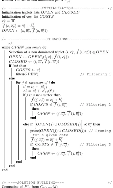
Data: A graph G = (V, A, T ), two vertices o, d ∈ V , two functions c and h, a departure date t0
Result: The set of non dominated paths P∗ od
/* ---INITIALIZATION--- */ Initialization triplets lists OP EN and CLOSED
Initialization of cost list COST S
− →co = −→0 − →f (o, −→c o) = −→co+ −→ho OP EN← (o, −→co, −→f (o, −→co)) /* ---ITERATIONS---*/
while OP EN non empty do
Selection of a non dominated triplet (i, −→ci, −→f (i, −→ci))∈ OP EN OP EN ← OP EN\(i, −→ci, −→f (i, −→ci))
CLOSED← (i, −→ci, −→f (i, −→ci))
if i=d then
COST S← −→ci
filter(OP EN) // Filtering 1 else
for j ∈ successor of i do
t"= t0+ [−→ci]1 −
→cj= −→ci+ −→cij(t")
if j is a new vertex then
− →f (j, −→c j) = −→cj+ −→hj if COST S ⊀ −→f (j, −→cj) // Filtering 2 then OP EN← (j, −→cj, −→f (j, −→cj)) end else if ! OP EN (j)∪ CLOSED(j) " ⊀ −→cj then
prune(OP EN(j) ∪ CLOSED(j)) // Pruning for a given date
− →f (j, −→c j) = −→cj+ −→hj if COST S ⊀ −→f (j, −→cj) // Filtering 3 then OP EN← (j, −→cj, −→f (j, −→cj)) end end end end /* ----SOLUTION BUILDING---- */ Computing of P∗ odfrom Cclosed(d)
Fig. 1: The new algorithm NAMOA*-T
Heuristics.: To ensure practical efficiency, we propose a
heuristic that is pre-computed before the algorithm. This heuristic must be a lower bound of the total cost between each vertex and the arrival one. It is a labelling procedure, that associates labels to each vertex. The heuristic gathers two subroutines, one routine for each element of the cost vector (more generally n subroutines for n-dimension cost vectors). For each subroutine, the heuristic algorithm is a Dijkstra algorithm starting on the arrival vertex, for which the arc cost is the minimal cost over the dates of the time space. This heuristic has the advantage to be independent of the problem application. We will see in the experiment section that it spends most of the total algorithm time: once the lower
Fig. 2: A graph representing possible moves on the sea. Each intersection of the grid matches a vertex. The nearest vertices are linked by bidirectional arcs.
bound is known for each vertex, NAMOA*-T is extremely fast. This is due to the fact that data access duration is quite a heavy operation, and has not been optimized for now.
IV. EXPERIMENTS
In this section, we assess the practical interest of our approach. We will compare the new NOAMA*-T algorithm with the best algorithm for this problem in the state of the art, the Veneti algorithm [24]. Both algorithms are implemented
inside an Atos1 internal tool. The comparison is done on real
data (map, weather forecast).
A. Time Dependent MSPP for Route Optimization of Cargo Ships
We consider here the problem of cargo ships routing optimization when the cost of the path can be dynamically modified due to the modification of the weather. To represent this problem, we need to use time dependent graphs. All the models of the state of the art are divided into two parts: discrete time models and continuous time models. The weather data provided as an input to our model are discrete data. For example,
we collect GRIB2files containing weather forecast information
on winds, currents, every 6 hours. To be consistent with the weather forecast sources, we chose a discrete time mathematical model (as described in II-A). In addition, cargo engines do not tolerate low speeds. Since the ship cannot move below a given speed (and moving in circle would cause time and fuel wastes), we do not consider the possibility of waiting at a vertex (e.g. for conditions weather to improve).
The vertices represent geographical locations and arcs possible moves between these vertices (the allowed moves are defined
a priori). The arcs of the graph are bidirectional (it contains directed cycles), and an arc cost is not necessarily equal to the reciprocal arc. Arc weights are positive (time, fuel consumption, various risks,. . . ) which limits the difficulty of the problem as negative cost cycles cannot exist. An example is given in fig. 2 (A is Rio de Janeiro while B is Cape Town).
The search can be launched on various types of graph: for the experiments, the two most accurate graphs are the 8-arcs
graph, and the 16-arcs graph. They correspond to a grid in
1Atos is a European IT services corporation which finances this project. 2GRIB is a concise data format commonly used in meteorology.
which each vertex is linked to the 8 (resp. 16) other nearest vertices, as represented in fig. 3.
Fig. 3: 16-arcs graph (left) and 8-arcs graph (right)
B. Data properties
The presented algorithm is justified by the data property. In this section two figures illustrate this property. The two graphs in fig. 4 and fig. 5 represent the density of arcs weights over all the arcs of the graph and all the dates of a GRIB file.
Fig. 4: Density graph (duration) for the arc weights.
Fig. 5: Density graph (fuel consumption) for the arc weights. Figure 4 represents the duration in seconds, whereas fig. 4 the fuel consumption in tons. First of all, we note that there are two density peaks. This is explained by the arc length. These data where collected on a 8-edges graph (cf section IV-C): in this graph, two sizes of arcs exist. The shortest one are the horizontal and vertical one, whereas the longest are the diagonal one (see fig. 3, 8-arcs on the right). We can see on
this figure that these latter one are √2 longer than the shorter
one: it is confirmed by the density figure. To have an idea of the density, we must focus on one peak.
If we look the first peak (on the left) of the fuel chart, we observe the major part of the values are included in the interval [150-200] tons.
As for the duration chart, the first peak shows that most of the values are included in [50 000-80 000] seconds (or [14-22] hours).
The ratio between these two values is lower than two, which reveals the low dispersion of the data over the average. The lower bound computed in NAMOA*-T is based on the shortest
paths with the minimal values of the time horizon. As data have a low standard deviation, we deduce that these minimal values are close to the real value, which explains why the heuristic is so accurate. This is why NAMOA*-T is powerful for this problem.
C. Experimental Protocol
The experiments have been performed on Linux CentOS 6.5 with two Intel(R) Core(TM)2 Duo CPU processors E6550 2.33 GHz and 3,8 Gio of memory, and the tool and the two algorithms are implemented in Java. For each instance, the solving is performed within a timeout of 60 minutes. Atos internal tool allows to retrieve online meteorological real-time data files (GRIB) all around the world, and then to launch a search between two coordinates of the world, so as to optimize various criteria. The cost functions useful to compute the fuel consumption and the time depending on weather information were implemented by experts. The test are running on the 8-arcs graph and the 16-arcs graph (fig. 3). Some parameters can be adjusted like the size of the graph for computation, and the data sources. The wind data source is used for computing the cost function as it is one of the most influential on the fuel consumption and time criteria. The grid is built by dividing up the earth with 2450 vertices, every single one separated by an equal space to its 4 nearest neighbours. The selected time granularity is 15 minutes, which means that we judge that more precision would not be coherent with the accuracy of the cost functions. The two algorithms include a common pre-computation phase that compute the shortest path following each criteria. For each criteria cost, the maximal tolerated value equals 1.5 times the cost of the pre-computed path. Beyond this cost, the potential path is considered as not relevant. The search is launched between coordinates pairs that represent main sea routes. Selected instances are associated to shipping lines. The busiest container ports have been selected for the tests. These main crossing points are represented on the map appendix A.
The table in appendix B represents the correlation between the crossing point name, its coordinates and its identifier on the map. The table in appendix C contains the id pairs that have been used as instances for computing multiobjective shortest paths. 27 ports pairs are evaluated in both directions, which means 54 sea routes. The aim of this experiment is to evaluate realistic use cases with real sea routes and real weather conditions, so as to compare the quality of the algorithm in these industrial conditions, and their match with the specific weather routing problem.
D. Reference algorithm: Veneti [24]
This label algorithm iterates over all time instances t from
departure date t0 to the maximal arrival date tmax. For each
date, it keeps a list L of vertices reached at this date associated to the cost of the partial path. When the iteration arrives at date t, the elements of the list associated to t are expanded at their turn. When a new triplet (date; vertex; cost) is found, it checks that no other triplet with the same (date; vertex)
pair has a better cost (strict dominance in the pareto meaning). If not, it can be added to the list L. This is the equivalent to our pruning procedure. Veneti’s algorithm iterates on dates whereas NAMOA*-T iterates on costs.
E. Results and Analysis
In fig. 6 we see that NAMOA*-T is really quicker than Veneti’s algorithm. E.g., when it lasts more than ten minutes, NAMOA*-T ends in less than 30 seconds (extreme point of the graph). The only instances where Veneti’s algorithm is quicker than NAMOA* are easy instances with few vertices which are solved really quickly. This is explained by the computation duration of the heuristic whose use is not relevant below a minimal problem size.
Fig. 6: Comparison of the two algorithms
Figure 7 and fig. 8 give theaverage results for each graph
(8-arcs and 16-(8-arcs) over the 54 instances presented in section C. The first column contains the algorithm (N. for NAMOA*-T and V for Veneti algorithm). In section II-A, the input data
of the problem are defined as a graph G = (V, A, T, −→c ).
Consequently, the problem size is function of the vertices number |V |, the arc number |A| and the number of dates |T |. Column 2 contains this last number (average over all instances). Actually, this value is precomputed before the algorithm starts, as explained in section IV-C. Column 3 represents the average of algorithm total duration while column 4 contains the data access duration (average percentage of total time). This percentage is quite low and regular for both algorithms which ensures that data processing does not fill the main part of the computation time. Column 5 is the average duration of the NAMOA*-T heuristic (in percent) over the tested instances. The heuristic computation fills 90% of the total algorithm duration: NAMOA*-T without the heuristic is very fast. It would be relevant to test this algorithm with quicker heuristics. In column 6, the average number of explored vertices shows that with this heuristic, NAMOA*-T visits 65% less vertices than Veneti’s algorithm. This is due to the filtering and pruning phases, and to the exploration order (by costs whereas Veneti is ordered by dates). Concerning the number of Pareto optimal
solutions, it is ranged from 1 to 16: it is not an exponential function of the number vertices, so that finding all of them stays relevant. This is explained by the data: arc costs have a low dispersion around the average. The high performance of our algorithm can be explained by the distribution of the costs: the low cost dispersion explains heuristic accuracy. It implies that filtering procedure is extremely powerful for this problem. Moreover, the exploration order is done on the estimated cost (with the heuristic), which guarantees to find quickly some first solutions, and these solutions are the base of the filtering procedure.
1 2 3 4 5 6
Algo. # of Total Data Heuristic Expl. vertic.
dates time (s) access /tot. numb.
N. 1330 2,99 7,2% 91,1% 59/2450
V. 1330 148,78 6.6% - 181/2450
Fig. 7: Table of average results over the 54 instances, in the 8-arcs graph.
1 2 3 4 5 6
Algo. # of Total Data Heuristic Expl. vertic.
dates time (s) access /tot. numb.
N. 1261 5,06 7,0% 90,9% 74/2450
V. 1261 211,76 6,7% - 189/2450
Fig. 8: Table of average results over the 54 instances, in the 16-arcs graph.
V. CONCLUSION
In this paper, we proposed a new algorithm called NAMOA*-T to solve the multiobjective shortest path problem in a time dependent graph. Our motivation to solve this problem is related to the optimization of fuel consumption and time for cargo ships following the weather forecast data. NAMOA*-T takes into account the features of the weather routing problem. We compared NAMOA*-T with the best algorithm known in the literature and proposed by A. Veneti in [24]. Our experiments are carried out in an internal optimization tool, with real-time weather forecast data (as in the targeted industrial use). They are conducted on 54 different instances. The results are very good, first of all because NAMOA*-T computes results quicker than Veneti’s algorithm, but above all, the computation
time seems to perfectly match the customer demand3, namely,
a computation time of approximately a few minutes. This work opens new perspectives: we must implement and test different heuristics, particularly faster ones (even if they are less accurate). It could improve the whole computation time. Moreover, it is necessary to test this new algorithm with other data, to show its efficiency on a larger class of problems. For example, in road optimization, it is not excluded that the data
3This information has been collected with two international chartering
benefits from similar features (cost distribution): this algorithm would be efficient. Finally, some experiments could be done on problems with more than two objectives (like safety on shipboard for example).
ACKNOWLEDGMENT
This work has been funded by Atos and by the ANRT
(Association Nationale Recherche Technologie). REFERENCES
[1] Review of Maritime Transport. United Nations Conference on Trade and Development, 2013.
[2] K.A. Andersen A.J. Skriver. A label correcting approach for solving bicriterion shortest-path problems. 27:507–524, 2000.
[3] Reinhard Bauer and Daniel Delling. Sharc: Fast and robust unidirectional routing. Journal of Experimental Algorithmics (JEA), 14:4, 2009. [4] J. Brumbaugh and D. Shier. An empirical investigation of some bicriterion
shortest path algorithms,. European Journal of Operational Research, 43:216–224, 1989.
[5] I. Chabini. Discrete dynamic shortest path problems in transportation applications,. Transportation Research Record, 8:170–175, 1998. [6] J.N. Clmaco and E.Q. Martins. On the determination of the nondominated
paths in a multiobjective network problem. Operations Research, 40:255– 258, 1981.
[7] Kenneth L Cooke and Eric Halsey. The shortest route through a network with time-dependent internodal transit times. Journal of Mathematical
Analysis and Applications, 14(3):493 – 498, 1966.
[8] S. E. Dreyfus. An appraisal of some shortest path algorithms. 17(3):395– 412, 1969.
[9] J.L. Santos E.Q. Martins. An algorithm for the quickest path problem,.
Operations Research Letters, 20:195–198, 1997.
[10] Michael R. Garey and David S. Johnson. Computers and Intractability:
A Guide to the Theory of NP-Completeness. W. H. Freeman & Co., New
York, NY, USA, 1979.
[11] Robert Geisberger, Peter Sanders, Dominik Schultes, and Daniel Delling. Contraction hierarchies: Faster and simpler hierarchical routing in road networks. Experimental Algorithms, pages 319–333, 2008.
[12] Andrew V Goldberg, Haim Kaplan, and Renato F Werneck. Reach for a*: Efficient point-to-point shortest path algorithms. In 2006 Proceedings
of the Eighth Workshop on Algorithm Engineering and Experiments (ALENEX), pages 129–143. SIAM, 2006.
[13] Tristram Grbener, Alain Berro, and Yves Duthen. Time dependent multiobjective best path for multimodal urban routing. Electronic Notes
in Discrete Mathematics, 36:487 – 494, 2010.
[14] H.W. Hamacher, S. Ruzika, and S.A. Tjandra. Algorithms for time-dependent bicriteria shortest path problems. Discrete Optimization, 3(3):238 – 254, 2006.
[15] P. Hansen. Bicriterion path problems. In Gnter Fandel and Tomas Gal, editors, Multiple Criteria Decision Making Theory and Application, volume 177 of Lecture Notes in Economics and Mathematical Systems, pages 109–127. Springer Berlin Heidelberg, 1980.
[16] J.M.J. Journe and J.H.C. Meijers. Ship routeing for optimum performance.
Transactions IME, February 1980.
[17] E. Kanoulas, Y. Du ane T. Xia, and D. Zhang. Finding fastest paths on a road network with speed patterns. Data Engineering, 2006. [18] D.E. Kaufman and R.L. Smith. Fastest paths in time-dependent networks
for intelligent vehicle-highway systems application. Journal of Intelligent
Transportation Systems, 1:1–11, 1993.
[19] Michael M. Kostreva and Malgorzata M. Wicek. Time dependency in multiple objective dynamic programming. Journal of Mathematical
Analysis and Applications, 173(1):289–307, February 1991.
[20] X. Gandibleux M. Ehrgott. Multiple Criteria Optimization. State of the Art Annotated Bibliographic Surveys, Boston, 2002.
[21] L. Mandow and J.L. Perez De La Cruz. A new approach to multiobjective a* search. In Proceedings of the XIX International Joint Conference on
Artificial Intelligence, 2005.
[22] E.Q. Martins. On a multicriteria shortest path problem. European Journal
of Operational Research, 16:236–245, 1984.
[23] John Mote, Ishwar Murthy, and David L. Olson. A parametric approach to solving bicriterion shortest path problems. European Journal of
Operational Research, 53(1):81 – 92, 1991.
[24] A. Veneti, C. Konstantopoulos, and G. Pantziou. Continuous and discrete time label setting algorithms for the time dependent bi-criteria shortest path problem. Computing Society Conference, pages 62–73, 2015. [25] P. Vincke. Problmes multicritres. Cahiers du Centre d’Etudes de
Recherche Oprationelle, (16):425439, 1974. APPENDIXA
WORLD MAP WITH MAIN PORTS OR CROSSING POINTS
APPENDIXB
CORRELATION CROSSING POINTS AND COORDINATES Id Port/crossing point Coordinates
1.1 Gibraltar Ouest 36 ˚ 00’21”N, 011 ˚ 51’54”W 1.2 Gibraltar Est 38 ˚ 35’02”N, 001 ˚ 29’38”E 2 Suez Canal 31 ˚ 33’09”N, 032 ˚ 46’59”E 3 Rotterdam 55 ˚ 41’36”N, 003 ˚ 22’08”E 3.1 West Manche 49 ˚ 35’58”N, 007 ˚ 24’43”W 4 Cape of Good Hope 43 ˚ 12’46”S, 020 ˚ 42’46”E 5 NY and new Jersey 39 ˚ 45’21”N, 070 ˚ 27’32”W 6 New Orl./Houston 26 ˚ 51’54”N, 089 ˚ 54’43”W 6.1 New Orl./Houston 2 24 ˚ 31’17”N, 075 ˚ 50’58”W 7 LA 31 ˚ 05’02”N, 120 ˚ 36’54”W 8 Tubarrao (Brasil) 29 ˚ 37’08”S, 047 ˚ 15’21”W 8.1 Est Brasil 06 ˚ 53’04”S, 032 ˚ 01’17”W 9.1 Singapore Ouest 06 ˚ 56’36”N, 093 ˚ 22’08”E 9.2 Singapore Est 00 ˚ 50’58”N, 107 ˚ 25’53”E 10 Shangai 27 ˚ 05’58”N, 129 ˚ 55’53”E 11 North-Est Asia 40 ˚ 41’36”N, 147 ˚ 44’38”E 12 Dampier (Australia) 16 ˚ 01’31”S, 119 ˚ 09’01”E 13 Gulf of Aden 14 ˚ 26’36”N, 054 ˚ 13’42”E 14 North-Ouest Africa 13 ˚ 44’24”N, 019 ˚ 35’58”W 15 Panama Canal Est 13 ˚ 02’13”N, 079 ˚ 21’54”W 15.1 Panama Canal Ouest 06 ˚ 28’28”N, 087 ˚ 48’09”W 16 Vancouver 46 ˚ 47’13”N, 127 ˚ 38’47”W
APPENDIXC
ID PAIRS THAT REPRESENT AN INSTANCE(SHIPPING LINE)
Origin-destination pairs (1/4) Orig. 8.1 5 5 3.1 3.1 6.1 8.1 Dest. 1.1 1.1 3.1 3 1.1 1.1 1.1 Origin-destination pairs (2/4) Orig. 5 8 8.1 14 8.1 13 9.2 Dest. 8.1 4 3.1 4 8 9.1 10 Origin-destination pairs (3/4) Orig. 11 7 16 4 6.1 7 Dest. 7 15.1 15.1 13 8.1 16 Origin-destination pairs (4/4) Orig. 16 14 12 10 1.1 14 4 Dest. 11 8.1 13 11 14 4 9.1