Competition and the Ratchet Effect

HAL Id: halshs-00333590

https://halshs.archives-ouvertes.fr/halshs-00333590

Submitted on 23 Oct 2008

HAL is a multi-disciplinary open access archive for the deposit and dissemination of sci-entific research documents, whether they are pub-lished or not. The documents may come from teaching and research institutions in France or abroad, or from public or private research centers.

L’archive ouverte pluridisciplinaire HAL, est destinée au dépôt et à la diffusion de documents scientifiques de niveau recherche, publiés ou non, émanant des établissements d’enseignement et de recherche français ou étrangers, des laboratoires publics ou privés.

To cite this version:

Gary Charness, Peter Kuhn, Marie Claire Villeval. Competition and the Ratchet Effect. Journal of Labor Economics, University of Chicago Press, 2011, 29 (3), pp. 513-547. �halshs-00333590�

Groupe d’Analyse et de Théorie

Économique

UMR 5824 du CNRS

DOCUMENTS DE TRAVAIL - WORKING PAPERS

W.P. 08-28

Competition and the Ratchet Effect

Gary Charness, Peter Kuhn, Marie Claire Villeval

Octobre 2008

GATE Groupe d’Analyse et de Théorie Économique UMR 5824 du CNRS

93 chemin des Mouilles – 69130 Écully – France B.P. 167 – 69131 Écully Cedex

Tél. +33 (0)4 72 86 60 60 – Fax +33 (0)4 72 86 60 90 Messagerie électronique gate@gate.cnrs.fr

Competition and the Ratchet Effect

Gary Charness, Peter Kuhn & Marie Claire Villeval

October 19, 2008

Abstract: The ‘ratchet effect’ refers to a situation where a principal uses private

information that is revealed by an agent’s early actions to the agent’s later disadvantage, in a context where binding multi-period contracts are not enforceable. In a simple, context-rich environment, we experimentally study the robustness of the ratchet effect to the introduction of ex post competition for principals or agents. While we do observe substantial and significant ratchet effects in the baseline (no competition) case of our model, we find that ratchet behavior is nearly eliminated by labor-market competition; interestingly this is true regardless of whether market conditions favor principals or agents.

Keywords: Ratchet effect, competition, experiment, private information, labor markets JEL Classifications: C91, D23, D82, J24, L14

Acknowledgments: We would like to acknowledge Bentley MacLeod for useful

discussions that helped to inspire this paper, and seminar participants at the European meeting of the Economic Science Association in Lyon for helpful comments. We would also like to thank Dimitri Dubois for programming the experiment and Julie Rosaz for valuable research assistance.

Contact: Gary Charness, Department of Economics, University of California, Santa

Barbara, 2127 North Hall, Santa Barbara, CA 93106-9210. E-mail:

charness@econ.ucsb.edu. Web page: http://www.econ.ucsb.edu/~charness. Peter Kuhn, Department of Economics, University of California, Santa Barbara, 2127 North Hall, Santa Barbara, CA 93106-9210. E-mail: pjkuhn@econ.ucsb.edu. Web page:

http://www.econ.ucsb.edu/~pjkuhn/pkhome.html. Marie Claire Villeval, GATE, CNRS, University of Lyon, 93, Chemin de Mouilles, 69130, Ecully, France, and IZA, Germany. E-mail: villeval@gate.cnrs.fr. Web page: http://www.gate.cnrs.fr/perso/villeval/.

The ‘ratchet effect’ applies to a situation where a principal contracts with an agent for more than once, the agent takes a hidden action and has private information, and binding multi-period contracts are not enforceable. In such situations, the ratchet effect occurs when actions taken by the agent early in the relationship reveal information to the principal, which is then used by the principal to the agent’s disadvantage. Examples include the setting of production targets for branches of a multidivisional firm or of a nationalized economy (Weitzman 1980), the design of compensation systems for workers within firms (Gibbons 1987; Ickes and Samuelson 1987), contracting between a social-welfare-maximizing regulator and firms under his/her jurisdiction (Laffont and Tirole 1988, Dalen 1995)), managers’ incentives to innovate (Dearden, Ickes and Samuelson 1990), procurement contracting (Laffont and Tirole 1993), optimal income taxation (Dillen and Lundholm 1996), agricultural share contracts (Allen and Lueck 1999), the economics of corruption (Choi and Thum 2003), and environmental regulation (Puller 2006).

A common feature of the above models is the presence of pooling equilibria early in the principal-agent relationship. For example, in the case of worker compensation, able workers tend to mimic workers with less ability by restricting their output early in the employment relationship. This benefits abler workers by preventing the firm from extracting their rents later in the relationship, but is socially inefficient. Another, less well-known feature of existing ratchet models is their tendency to model agents’ participation constraints very simply, typically by requiring the utility of all agent types to exceed the same threshold in each period. While this may make sense in some cases (such as firms in nationalized economies) it may be unrealistic in other contexts, such as competitive labor markets where outside options may vary over time and—more importantly—across agent types.

The robustness of the ratchet effect to the competitive environment is an important question in economics. For example, while ratchet effects may be common in centrally-planned economies, or in labor markets characterized by substantial mobility costs or firm-specific capital, the importance of ratchet effects in markets characterized by a high degree of competition and (at least potential) mobility is less clear. One model of ratchet effects that expands the treatment of agents’ outside (market) alternatives is Kanemoto and MacLeod

(1992).1 Kanemoto and MacLeod show that, even when the outside market does not observe the agent’s early-career performance, the presence of ex post market opportunities for agents can eliminate the ratchet effect, allowing first-best effort levels to be attained.2 This suggests that

ex-post markets for agents may be a more powerful force in eliminating ratchet effects than

previously realized.

Aside from some early ethnographic studies (see for example Mathewson 1931), the only empirical evidence of ratchet effects of which we are aware is experimental in nature, and none it of considers the effect of competition among principals or agents.3 Chaudhuri (1998) conducted a laboratory experiment in which principals and agents interacted for two periods, and agents were one of two types that were unobserved by the principal. There was little evidence of ratcheting: most agents played naively, revealing their type in the first period even when an

1 _{Another such model is Roland and Sekkat (2000), who consider a situation where agents’ first-period performance}

is observed by an outside labor market. Arguably, this puts Roland-Sekkat’s model into a different class of models from the ratchet-effect literature, often referred to as “career concerns” models (see for example Dewatripont, Jewitt and Tirole 1999). In addition to making agents’ output public information, career concerns models typically do not incorporate private information about an agent’s type. In contrast to ratchet-effect models, career-concerns models are capable of generating socially excessive effort early in the agent’s career.

2 _{Intuitively, this is because able agents are able to generate more total surplus from the employment relationship}

than less-able agents. Even when the market does not observe first-period performance, this generates type-specific participation constraints in the second period, which protect able agents from exploitation. Note that this reasoning does not apply to the case modeled by Gibbons (1987), where the asymmetric information applies to the firm’s technology rather than the agent’s type.

3 _{An exception is Allen and Lueck (1999), who use cash rent and cropshare contract data to test for the presence of}

the ratchet effect in the context of moral hazard in agricultural contracts, but they do not consider the role of competition. They find limited evidence for the ratchet effect within share contracts and conclude that it cannot explain the choice of contracts.

informed principal would use this information to the agent’s disadvantage, and principals often did not exploit agents’ type revelation. Possible explanations for this result include the relative complexity of the game, and the lack of context provided to the subjects that might have impeded the learning process.

The only other experimental study of the ratchet effect of which we are aware is Cooper, Kagel, Lo and Gu (1999). Cooper et alii frame their experiment in a context-rich way, as a game between central planners and firm managers, use both students and actual Chinese firm managers as subjects, and are able to implement experimental payoffs with high stakes relative to the participants’ real-world incomes. They also simplify the interactions between principals and agents, focusing the experiment only on the stages of the game where information revelation matters: the agent’s effort choice in the first period, and the principal’s choice of a payoff schedule in the second. Cooper et alii do find evidence of ratchet effects, though even in their context it took some time for the players to learn the consequences of type revelation.

This paper reports the results of some simple laboratory experiments on the ratchet effect, in the context of piece-rate compensation. It differs from existing experimental studies in two main ways. First, motivated by Kanemoto and MacLeod’s theoretical insight, we introduce market competition for agents and principals, by allowing players to choose between their current partner and an alternative partner at the start of each stage of the game.4 Second, motivated by the Cooper et alii experimental approach, we simplify the interactions between principals and agents even further. Specifically, we focus only on the strategic interactions at the

4 _{We are aware of only two other principal-agent experiments that include treatments featuring both excess firms}

and excess workers. Brandts and Charness (2004) find only minor effects on the ratio of ‘effort’ to ‘wage’, according to the direction of market imbalance in a gift-exchange experiment, and also find deleterious effects on effort when a minimum wage is introduced. Cabrales, Charness, and Villeval (2006) show that in a static game with informational asymmetry and hidden information, inefficiencies remain when principals compete against each other to hire agents. In contrast, when agents compete to be hired, efficiency improves dramatically, and it increases in the relative number of agents because competition reduces the agents’ informational monopoly power.

heart of the ratchet effect, i.e. those between the high-ability agents’ first stage efforts and the principals’ second-stage rewards, and we reduce both parties’ strategy sets to two choices (high or low effort, and high or low pay). Combining this with a simple context that makes sense to our subjects (principals are firms and agents are workers), we believe that this significantly improves our subjects’ understanding of the game.

Our main findings are twofold. First, we observe substantial and significant ratchet effects in the baseline case of our model (which, like Chaudhuri and Cooper et alii, does not incorporate ex post labor market competition). We believe that this is in large part due to our simpler design that focuses on the main strategic issues. Second, we find that ratchet behavior is significantly reduced by labor-market competition; interestingly this is true regardless of whether labor-market conditions favor workers (our ‘excess firms’ case), or firms (our ‘excess workers’ case). In the excess-firms case, it appears (as Kanemoto and MacLeod’s analysis predicts) that talented workers are not reluctant to reveal their types in the first stage, because they can escape the incumbent firm’s desire to exploit them ex post. In the excess-workers treatment, workers cannot be sure they will be matched with any firm, let alone the current one, in the second stage. This also reduces talented workers’ incentives to hide their types in the first stage; on the

contrary (for reasons that evoke the ‘career concerns’ literature), they are willing to reveal their type in order to keep a contract in the second stage.

Overall, our results suggest that the ratchet effect is highly vulnerable to market competition, even when (as is traditionally assumed in ratchet models, and as is true in all our experimental treatments) incumbent firms have an informational advantage over outside firms. Agents’ effort levels, and the joint surplus generated by the employment contract, are therefore increased in the presence of competition. Thus, it appears that either institutional barriers to

competition among both agents and principals, or a high level of relationship-specific

investments, may be more important to the existence of ratchet effects than previously realized.

2. A Model

Let worker utility be given by U= w !"V (e), where w is total compensation and!V (e)

is the cost of effort, e. V (e) has the usual form (V (0)= 0, ! V > 0, ! ! V > 0); we shall use V (e)= e2

to generate parameter values for the experiment. There are two types of workers, high and low ability (or “talent”), differentiated by their effort costs, !H _< !L_{. Output is given by the}

production function y= e; since this is the same for both workers we henceforth use y

exclusively to denote both output and effort. Firms’ profits are given by ! = y " w. Firms offer piece rate contracts of the form w= !"+#y to workers. In fact, we set !=1, since this achieves

the first best in a full information environment. This means that firms’ only decision is over the value of !. One interpretation of ! " 0 is as the ‘entry’ fee the firm charges the worker for the right to use its plant and equipment; as is well known when !=1 these fees will constitute the firm’s only source of profit.5

Under the above conditions, the socially optimal output levels are given by y= 1

2!. With

!=1 these are also the output levels that we expect workers to choose in a one-stage interaction with firms, as long as the level of ! satisfies both workers’ participation constraints. High-talent workers will produce more output than low-ability workers; in consequence both workers’ types are revealed and a first-best outcome is attained.

5 _{Although explicit job entry fees are rarely observed in reality (and are in some cases illegal), it is well known that a}

variety of contracting mechanisms are equivalent to these fees. One example is a positive level of “base” compensation combined with a minimum output quota that must be reached in order to qualify for a piece rate; in this interpretation a higher entry fee (α) corresponds to a higher output quota. Note also that the 100% piece rates assumed here refer to 100% of the firm’s net revenues, not of gross sales. See Lazear 1998, chapter 5 for a discussion.

Now imagine that workers and firms engage in a two-stage interaction, with the stages of potentially different length. The worker’s type is still unknown to the firm at the start of the first stage, but the firm now might infer something about it from the worker’s stage-one output. In particular, high stage-one output might signal high worker ability, implying that the firm can charge a higher entry fee in stage two without violating the worker’s participation constraint. Anticipating this, high-ability workers might ‘masquerade’ as low-ability workers in the first stage. As a result, firms will continue to offer the low entry fee in the second stage, since they were unable to identify the worker’s type in the first stage. Thus, we would observe inefficient pooling at the low output level in the first stage, especially if the first stage is short relative to the second.

Finally, suppose that at the start of the second stage, all workers can receive a competing wage offer from another firm. As Kanemoto and MacLeod (1992) have shown, this can prevent ‘incumbent’ firms from exploiting high-talent workers who reveal their type in the first stage, even when outside firms do not observe workers’ stage-one outputs. Our experiment tests this prediction, implementing the exact model described above with parameter values as described below.

In our experiment, we set !L _{= .010 and} !H _{= .005, which yields socially optimal output} levels of ( 1

2! =) 50 and 100 for the low- and high-talent workers respectively.

Throughout the experiment, we restrict workers’ output choices to these two levels, which we shall call ‘low’ and ‘high’ output respectively. Thus, if each worker type chooses his ‘type-appropriate’ output, a first-best outcome will be achieved. Asymmetric information-induced inefficiencies will take the form of workers choosing the type-inappropriate output level.

Workers receive a baseline payoff of zero if they do not work for any firm. If workers choose type-appropriate outputs, the total surplus generated by the employment relationship (e!"V (e)) is 25 and 50 respectively for the low- and high-talent workers respectively; 25 and 50 are thus the maximum entry fees the firm can charge each type of worker if it knows the

worker’s type. In our experiment, we will allow firms to choose between two entry fees only: !L _{= 15 (“low”) and !}H _{= 33 (“high”). We set the ex ante probability that a worker has high} ability at 1

3.

6 _{Finally, in our implementation, workers and firms interact over either one or two}

stages, with the second stage twice as ‘long’ as the first (thus all the payoffs listed above are doubled, and the entry fees adjusted accordingly at 30 and 66). As noted, raising the relative importance of the second stage raises workers’ incentives to manipulate the information the firm has about them in that stage.

Under the above assumptions, low-ability workers’ stage-one payoffs if the firm posts the low entry fee are 10 and -15 at low and high effort levels respectively; if the firm posts the high fee they are -8 and -33 respectively. Thus, in a one-shot game with no strategic interactions, we expect low-talent workers to choose low effort if the firm posts the low entry fee, and to refuse to work for the firm at the high entry fee. Similar calculations show that high-talent workers find it optimal to supply high effort regardless of the entry fee (though they are obviously better off at the low fee). Thus we would expect to observe an efficient separating equilibrium if the game has only one stage. However, in a two-stage game with no competition, a forward-looking high-talent worker might conceal his type in the first stage (thus sacrificing some current payoff) if he believes this will lead the firm to reduce its second-stage fee, leading to an inefficient pooling

6 _{If this probability is too high, a firm that does not know its worker’s type will optimally choose the high entry fee,}

thereby shutting low ability workers out of the market. Thus the pooling equilibrium at the heart of the ratchet model cannot exist. A value of 1/3 gives firms adequate incentives to set the low fee and retain both worker types when the worker’s type is unknown.

equilibrium. If one introduces competition between firms, a high-talent worker might again choose to reveal his type in the first stage because in the second stage the incumbent firm refrains from raising the fee to avoid the risk of losing its worker. Thus, between-firm

competition could restore efficiency by preventing firms from exploiting workers’ informational rents.

If the competition is between workers, high-ability workers have a different incentive to reveal their type in the first stage; namely their concern about not receiving a contract in the second stage (firms prefer to be matched with high-ability workers because they can extract more rents from them, especially when there are excess workers in the market). In this context, firms will find it easier to impose the high fee in the second stage. Thus we expect that in the presence of excess workers, a separating equilibrium can emerge in which firms are able to fully exploit the informational rent extracted from their ‘incumbent’ workers. In the experiment, we shall compare effort and entry fees in all four situations discussed above—a one-shot interaction; and two-stage interactions with no competition, competition among firms, and competition among agents—to see if all the above expectations are in fact confirmed.

3. Experimental design

Our experiment was conducted at the Groupe d’Analyse et de Théorie Economique (GATE), CNRS, France. The students were recruited from undergraduate courses in local Engineering and Business schools, by means of the ORSEE software (Greiner, 2004). In total, 159 people took part in the nine sessions (three for each treatment) of this experiment. Upon arrival of all the participants, each person was assigned a computer, by a draw from an opaque bag. No one could participate in more than one session, and the same experimenters conducted

all of the sessions. In each treatment, there was a conversion rate of 100 experimental units to €1. Average earnings were €14, including a €5 show-up fee.

Each participant was given the role of either a high-talent worker or a firm. The number of participants allocated to each category depended on the treatment. We decided to have automated low-talent workers, as their decisions were quite trivial (reject contracts with a high entry fee, as this would generate negative earnings for the worker, and accept contracts with low entry fees, since this provides positive earnings for both firms and workers.)7 Since we expected virtually no deviation from this strategy, we programmed the low-talent workers to follow it. It was made common information in the instructions that the low-talent workers were robots and that they were programmed to follow this strategy.8

In order to facilitate comprehension, we couched our experiment in terms of the firm being the owner of a food concession stand on campus.9 Note that the firm’s income is only what is received in rental fees. In the first part of a period (or first stage of the interaction), the firm is willing to rent the stand (to a worker) for one week; we restrict the firm to charging the low entry fee of 15 in order to provide a high-talent worker with a real choice, thus enabling us to gather useful data.10 If a firm or a worker does not end up in a contractual relationship, he or she receives nothing for that stage. If a high-talent worker accepts a contract, he or she chooses either low or high output, with the worker earning more in that stage from high output. Each firm is then informed about the output level (reject, low, or high) of the worker in the first stage,

7 _{Even negative reciprocity could not come into play with human low-talent workers, as the firm is not being}

antagonistic by choosing the lower entry fee.

8 _{The robots were programmed with different response times and one proceeded to the next step only once all the}

players had entered their decisions. Therefore, the only evidence that a firm had concerning the nature of the worker was the choice made by the worker.

9 _{We attempted to insure comprehension by requiring participants to complete a “Comprehension questionnaire,”}

which can be found in Appendix A, along with a sample of the experimental instructions.

10 _{Choosing the high fee of 33 gives an expected gain of only 11 for the firm in that stage. In addition, allowing the}

firm to choose the high fee in this stage would allow it to uncover the type of its worker but at the risk of having its offer rejected if matched with a low-talent worker. This would not test the ratchet effect.

but not the worker’s type.

In the second stage, the firm is free to choose either the low entry fee (30) or a high entry fee (66). Low-talent workers make their programmed choices, while high-talent workers choose to either reject the offer or to provide low or high output. In order to increase the cost of

inefficiencies, this second stage ‘lasted’ two weeks, rather than one week. Once again, firms were informed about the output chosen. Table 1 below presents the game and all possible payoffs. The main feature we wish to note is that if a high-talent worker chooses high output, he will receive 35 in the first stage, but will face a high rental fee if the firm realizes that she is matched with a high-talent worker, and will receive 34 in the second stage (so 69 in total). In comparison, the high-talent worker who chooses low output in the first stage earns 22.5 then and, if the firm subsequently chooses a low rental fee, earns 70 in the second stage (so 92.5 in total). Notice that, by construction, the choice of type-appropriate outputs by both worker types

Table 1 – The Game First stage

Worker’s type Rental fee Worker’s choice Firm’s payoff Worker’s payoff

Reject 0 0 Low output 15 22.5 High-talent 15 High output 15 35 Reject 0 0 Low output 15 10 Low-talent 15 High output 15 -15 Second stage

Worker’s type Rental fee Worker’s choice Firm’s payoff Worker’s payoff

Reject 0 0 Low output 30 45 30 High output 30 70 Reject 0 0 Low output 66 9 High-talent 66 High output 66 34 Reject 0 0 Low output 30 20 30 High output 30 -30 Reject 0 0 Low output 66 -16 Low-talent 66 High output 66 -66

Each session included five periods consisting of only the first stage in order to verify that the workers understand that the high-output choice is best when there is no continuation. The instructions for the dynamic game were distributed only after completion of these five periods. The participants played then 20 periods of the two-stage game, with firms and workers randomly re-matched in each new period.

Baseline treatment

We had equal numbers of firms and workers in this treatment. There were 20 live participants in two sessions and 16 in the third session due to no-shows. Fifteen participants

were assigned to be ‘firms’ and five participants were assigned to be ‘high-talent workers’; there were also 10 automated low-talent workers.11 Each firm is matched with one worker of

unknown type. There is no competition in this treatment, since the worker is paired with the same firm for both stages of every period.

Excess-firms treatment

We had twice as many firms as workers in this treatment, with 21 live participants in each session. Eighteen participants were assigned to be ‘firms’ and three participants were assigned to be ‘high-talent workers’. The other six workers were automated low-talent workers. In the first stage, each worker is paired with two firms. In the first stage, both firms make the offer of a low rental fee (15) to their paired worker. The worker chooses to accept at most one of these (identical) offers.

As before, the ‘incumbent’ firm learns the output level. In the second stage, both firms offer either a low or a high rental fee to the worker. If the worker accepts an offer, then he chooses either low or high output. If both offers involve the low rental fee, low-talent workers accept one at random; the high-talent worker is completely free to choose which (if either) offer to accept and to choose any output level. Indeed, the worker receives both offers at the same time and he can identify the firm with whom he contracted in the first stage.

Excess-workers treatment

We had twice as many workers as firms in this treatment, with 15 live participants in two sessions and 10 in the third session due to no-shows. Nine participants were assigned to be ‘firms’ and six participants were assigned to be ‘high-talent workers’ (respectively, six and four in the third session). The other 12 workers were automated low-talent workers. In the first stage, each firm is paired with two workers of unknown type. In the first stage, the firm makes

an offer to one of the two workers; if this worker rejects the offer, then the offer is made to the second worker. The second worker is not informed that the first worker has turned down the offer. As before, the firm learns the output level. In the second stage, the firm chooses either a low or a high rental fee and chooses to approach either the worker who had accepted the contract in the first stage or the other worker.12 _{Once again, if the offer is rejected, it is then made to the}

other worker.

4. Experimental results

Table 2 summarizes for each treatment the decisions made by the subjects in the five single-stage periods and then in each stage of the 20 two-stage periods.

Effort decisions

We first mention that high-talent workers appear to have understood the basic game in the five single-stage periods. High-talent workers rejected a low-fee contract offer in only two of 151 occasions (1.32%), and chose low output on five occasions out of 149 (3.36%). Thus, we see the predicted outcome an overwhelming proportion of the time in the static game with only one stage.

How do matters change when there are two stages? Table 2 shows the proportion of high-talent workers who chose the low output in the first stage, after having received an offer with a low rental fee.

12 _{In principle, if neither worker accepted the contract in the first stage, the worker who first received the offer in the}

Table 2 - Summary statistics Baseline (1) Excess firms (2) Excess workers (3) Total (4) Single-stage periods Rejected contracts Accepted contracts High output Low output Total 2 (2.94) 68 (97.06) 65 (95.59) 3 (4.41) 68 (100) 0 (0) 45 (100) 43 (95.56) 2 (4.44) 45 (100) 0 (0) 36 (100) 36 (100) 0 (0) 36 (100) 2 (1.32) 149 (98.67) 144 (96.64) 5 (3.36) 149 (100) Two-stage periods Stage 1 Rejected contracts Accepted contracts High output Low output Total 3 (1.07) 277 (98.93) 106 (38.27) 171 (61.73) 277 (100) 0 (0) 180 (100) 180 (100) 0 (0) 180 (100) 0 (0) 164 (100) 145 (88.41) 19 (11.59) 164 (100) 3 (0.48) 621 (99.52) 431 (69.40) 190 (30.60) 621 (100) Stage 2 - Offers

After a low output - High fee - Low fee After a high output

- High fee - Low fee Total 87 (11.90) 644 (88.10) 98 (92.45) 8 (7.55) 837 17 (4.72) 343 (95.28) 54 (30.00) 126 (70.00) 540 154 (46.11) 180 (53.89) 136 (93.79) 9 (6.21) 479 258 (18.11) 1167 (81.89) 288 (66.82) 143 (33.18) 1856 Stage 2 Rejected contracts Accepted contracts High output Low output Sum 6 (2.14) 274 (97.86) 265 (96.72) 9 (3.28) 274 (100) 0 (0) 180 (100) 180 (100) 0 (0) 180 (100) 20 (8.65) 211 (91.34) 211 (100) 0 (0) 211 (100) 26 (3.76) 665 (96.24) 656 (98.65) 9 (1.35) 665 (100) Stage 2 - Switches after

- High fee/output - Low fee/output No switch after - High fee/output - Low fee/output Total - - - - - 51 (48.57) 54 (51.43) 3 (4.00) 72 (96.00) 180 (100) 13 (9.42) 125 (90.58) 132 (38.71) 209 (61.29) 479 (100)

Note: Percentages are in parentheses. As far as the agents’ decisions are concerned, the table only reports those of the high-skill (human) agents. In the Excess workers treatment, the difference between the number of observations in stage 1 and in stage 2 is due to the fact that the firms do not necessarily offer contracts to the same agent in the two stages. In column 2, the decision to switch emanates from the agents; in column 3, it emanates from the firms; therefore, these numbers cannot be summed in column 4.

In the baseline treatment, we see considerable evidence that workers are aware of the problem with revealing that they have high talent by choosing the high output in the first stage. In fact, 171 of 277 times that a contract was accepted (61.73%),13 high-talent workers chose a low output, deferring immediate gains in favor of future benefits. This 61.73% contrasts greatly with the 4.41% low-output rate observed in the static game of this treatment. An analysis of the behavior of the 14 individual high-talent workers is revealing. In fact, there were four workers who always chose a high output, apparently failing to grasp the basic principle involved; one other worker acted almost randomly, choosing each of the high and low outputs nine times and rejecting the low-fee rental contract twice, suggesting some degree of confusion. The other nine workers rarely chose high outputs in the first stage, and these choices were generally made in the first periods of a session.

We can also compare these choices to those of the high-talent workers in the second stage, where (at least direct) strategic considerations are absent. In 265 of the 274 instances (96.72%) where a high-talent worker was offered a contract in the second stage, he chose a high output.14 _{This behavior is in stark contrast to the 38.27% likelihood of choosing the high output}

in the first stage, where the future looms large.15

Behavior changes greatly when there is competition between firms. High-talent workers accepted the contract offers and chose the high output in every one of the 180 instances when a high-talent worker was offered a contract in the first stage. It seems quite clear that, in line with the Kanemoto and MacLeod (1992) model, competition for scarce workers leaves high-talent

13 _{The contract was rejected (inexplicably, since doing so also reveals high talent) three times of 280 (1.07%).} 14 _{The contract was rejected six times (2.14%) and the low output was chosen nine times (3.28%). All six rejections}

were of the high-rental-fee contract. Strangely, eight of the nine choices of low outputs came after a low-fee contract was offered.

15 _{The average individual output is significantly higher in the second stage than in the first one in the baseline}

workers unafraid to reveal their type early in the game. What is perhaps more surprising is that the ratchet effect also vanishes when there is a scarcity of firms, so that workers compete with each other. High-talent workers always accept an offer, and they choose the low output in only 19 of 164 instances (11.59%) in the first stage.16 We conjecture that workers realize that firms would like to be able to charge the high rental fee, so that signaling high talent is useful for obtaining any offer in the second stage.17

Does high-talent workers’ behavior change over time? Figure 1 shows the proportion of time a low output was chosen by a high-talent worker, by five-period blocks.

Figure 1 - Low output rates over time, high-talent workers, first stage

48.28% 62.78% 68.12% _65.71% 0% _0% 0% 0% 7.50% 6.82% 9.76% 23.08% 0% 20% 40% 60% 80% 100% 1 to 5 6 to 10 11 to 15 16 to 20 Period % Baseline Excess firms Excess workers

16 _{An analysis of individual behavior shows that only four of the 16 high-talent workers in this treatment ever chose}

the low output in the first stage. One of these was responsible for 11 of the 19 low outputs observed.

17 _{While it seems obvious that the percentage of low outputs with high-talent workers in the first stage differs across}

treatments, we can also provide a very conservative nonparametric test that confirms statistical significance. The percentage of low outputs with high-talent workers in the first stage was 52%, 74%, and 59% in the three baseline sessions; these percentages were 0%, 0%, and 0% in the three sessions with excess firms, and 3%, 4%, and 25% in the three sessions with excess workers. Thus, the Wilcoxon rank-sum test finds significant differences (p = 0.050) in rates across any pair of treatments, using each session as only one independent observation. Taking the individual as a unit of observation, the mean output in the first stage is significantly lower in the baseline than in the excess-firms treatment (Wilcoxon test, p = 0.002) and than in the excess-workers treatment (p = 0.001). There is no significant difference in this respect between the excess-firms and the excess-workers treatments (p > 0.100).

In the first ten periods of the baseline, the proportion of strategic low outputs increases sharply and then remains almost stable, suggesting a strong learning effect. In contrast, there is a sharp increase in the last five periods in the proportion of low outputs chosen in the excess-workers treatment, but this emanates from only two participants out of 16.18 In any case, the difference in the likelihood a high-talent worker will hide his type is strong across treatments, regardless of the time period under consideration.

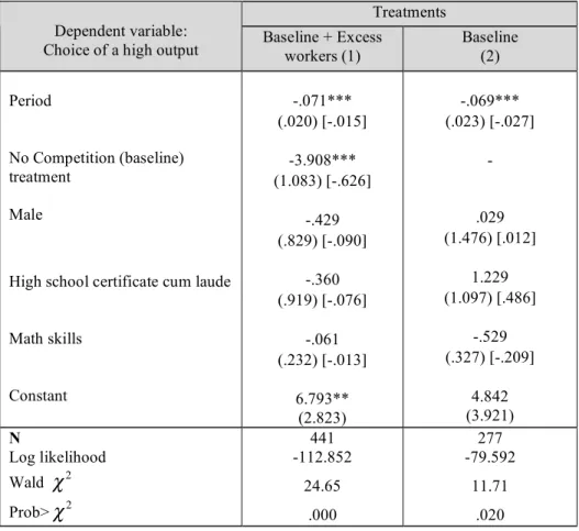
We estimate a random-effects Probit model to identify the determinants of the choice of a high output in the first stage of the game, since several decisions are made by the same

individuals. The independent variables include the treatment, a time trend, and individual characteristics, namely gender and cognitive abilities proxied by the level obtained on the final high-school exam and by the mark obtained in mathematics in this exam. Table 3 displays the results of these estimations for pooled data (column 1) (excluding the excess firms treatment since all subjects chose the high output) and the baseline treatment alone (column 2).

Table 3 confirms that, in the first stage, the high-talent workers choose the high output significantly less frequently in the baseline treatment than in the excess-workers treatment (and a

fortiori than in the excess-firms treatment). The time trend is also highly significant, suggesting

that subjects learn to play strategically in the baseline. The individual characteristics are not significant; it should however be noted that in the baseline, the ability in mathematics exerts a borderline influence (significant at the 10.6% level with a two-tailed test). Intuitively, higher mathematical ability favors strategic reasoning.

18 _{The average individual output is marginally-significantly lower in the last ten periods than in the first ten periods}

Table 3 - Determinants of a worker choosing the high output in the first stage (Random-effects Probit model)

Treatments Dependent variable:

Choice of a high output Baseline + Excess _{workers (1)} Baseline ₍₂₎ Period

No Competition (baseline) treatment

Male

High school certificate cum laude Math skills Constant -.071*** (.020) [-.015] -3.908*** (1.083) [-.626] -.429 (.829) [-.090] -.360 (.919) [-.076] -.061 (.232) [-.013] 6.793** (2.823) -.069*** (.023) [-.027] - .029 (1.476) [.012] 1.229 (1.097) [.486] -.529 (.327) [-.209] 4.842 (3.921) N Log likelihood Wald !2 Prob>!2 441 -112.852 24.65 .000 277 -79.592 11.71 .020 Standard errors are in parentheses and marginal effects are in brackets.

*** means significant at the 0.01 level, ** at the 0.05 level.

Choice of rental fees

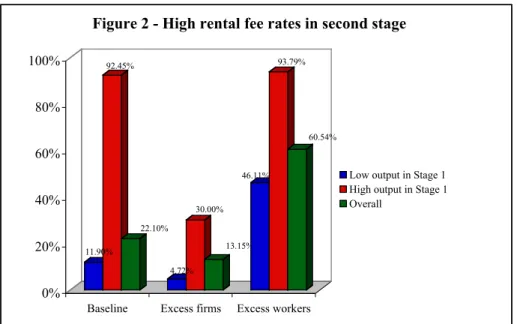
We next consider the behavior of the firms. Figure 2 shows the choices of rental fees by firms in the second stage, both overall and also according to whether the paired worker chose a high or low output level in the first stage.

11.90% 92.45% 22.10% 4.72% 30.00% 13.15% 46.11% 93.79% 60.54% 0% 20% 40% 60% 80% 100%

Baseline Excess firms Excess workers

Figure 2 - High rental fee rates in second stage

Low output in Stage 1 High output in Stage 1 Overall

Firms were much more likely to choose a high rental fee in the second stage after learning of a high output in the first stage; this was true in all treatments. In contrast, the proportion of firms offering the high fee is significantly different across treatments.19

In the baseline treatment, firms overall chose the high rental fee 22.10% of the time; the rate after a high output was observed was 92.45%, but was only 11.90% after a low output was observed. Thus, it may be that some firms fear rejection if a high fee is proposed, while a few firms are willing to take a chance that it was a high-talent worker who chose the low output in the first stage. Overall, this confirms the rationality of high-talent workers who choose to conceal their ability in the first stage.

When there are excess firms, firms choose a high rental fee in the second stage only 13.15% of the time; the rate after a low output was observed was only 4.72%, but was 30% after a high output was observed. Recall that high-talent workers always chose high outputs,

appearing to believe that they can reveal their type with impunity. At first glance, the 30% rate

19 _{Averaging values by individual and considering each individual as an observation, Mann-Whitney tests conclude}

that firms propose higher fees in the baseline than in the excess-firms treatment (p < 0.001) and that firms in the excess-workers treatment offer higher fees than in both the excess-firms (p < 0.001) and the baseline treatments (p < 0.001).

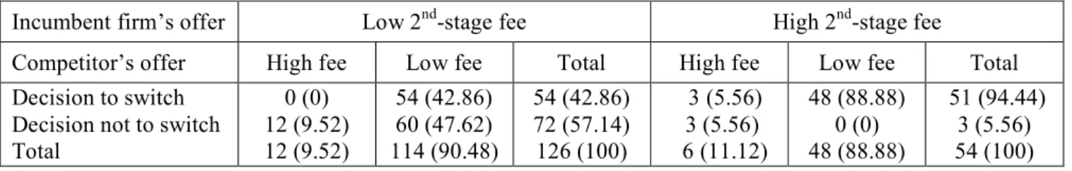
after a high output appears to be a serious consequence of revelation; however, since the worker was paired with two firms, there was also the chance that the other firm would offer a low rental fee. In fact, after revealing high talent in the first stage, the high-talent worker nevertheless received at least one offer with low rental fees in the second stage in 174 of 180 cases (96.67%), so choosing high output in the first stage was rarely costly in fact. The analysis of the workers’ switching decisions between firms is also informative. Table 4 displays the workers’ decisions depending on the second stage fees chosen by the incumbent firm and its competitor.

Table 4 - Decisions to switch firms in the second stage, excess-firms treatment

Incumbent firm’s offer Low 2nd_{-stage fee High 2}nd_{-stage fee}

Competitor’s offer High fee Low fee Total High fee Low fee Total

Decision to switch Decision not to switch Total 0 (0) 12 (9.52) 12 (9.52) 54 (42.86) 60 (47.62) 114 (90.48) 54 (42.86) 72 (57.14) 126 (100) 3 (5.56) 3 (5.56) 6 (11.12) 48 (88.88) 0 (0) 48 (88.88) 51 (94.44) 3 (5.56) 54 (100)

Note: Percentages are in parentheses.

This table shows that it never pays for a firm to choose the high rental fee in the second stage since doing so leads the agent to select the contractual offer of the competitor. When both firms choose the high fee, the workers are indifferent.20 _{In a random-effects Probit model}

analyzing the workers’ probability to switch firms (not reported here but available upon request), we find that being matched with two firms choosing a high fee reduces the likelihood that the worker switches firms by 41.83 percentage points, while being matched with two firms choosing the low fee reduces this likelihood by 32.70 percentage points.

The picture is somewhat different with excess agents, where high rental fees were chosen overall 60.54% of the time. Now workers are more desperate to find employment, and revealing high talent has strategic value. Indeed, the firms capitalize on the information, as firms in this

20 _{Interestingly, we do not find clear evidence of inequity aversion. Indeed, inequity-averse workers would switch}

position chose the high rental fee 93.79% of the time in the second stage. So here the firms capture the lion’s share of the available rents. When firms learn of low output in the first stage, they are uncertain of the right course of action, and the low rental fee is chosen in the second stage 46.11% of the time. Here again, the analysis of switching decisions is informative. Table 5 reports descriptive statistics on the firms’ decisions to switch agents between the first and the second stages.

Table 5 - Decisions to switch workers in the second stage, excess-agents treatment

Firm learns the worker has high talent Firm does not learn the type of its agent

Second stage fee High fee Low fee Total High fee Low fee Total

Decision to switch Decision not to switch Total 10 (6.90) 126 (86.90) 136 (93.79) 3 (2.07) 6 (4.14) 9 (6.21) 13 (8.97) 132 (91.03) 145 (100) 66 (19.76) 88 (26.35) 154 (46.11) 59 (17.66) 121 (36.23) 180 (53.89) 125 (37.43) 209 (62.57) 334 (100)

Note: Percentages are in parentheses

Nearly eight-seven percent of the firms who learn that the worker with whom they were matched in the first stage has high talent propose the high fee in the second stage to the same worker. In a random-effects Probit model analyzing the firms’ probability to switch workers (not reported here), we find that being matched with a worker choosing a high output in the first stage reduces the likelihood that the firm switches workers in the second stage by 31.79

percentage points. Decisions are less simple when the firms have not learned with certainty the type of their worker. 17.66% of these firms propose the low fee to the other worker and 36.23% to the same worker; 19.76% propose the high fee to the other worker and 26.35% to the same worker. These latter are the less rational decisions since in the first case, it suggests an overestimation of the probability to meet another high-talent agent, and in the second case, a

high-talent worker has no reason to hide his type in the first stage. This may be due to confusion or to high expectations regarding the probability of meeting a high-talent worker. 21

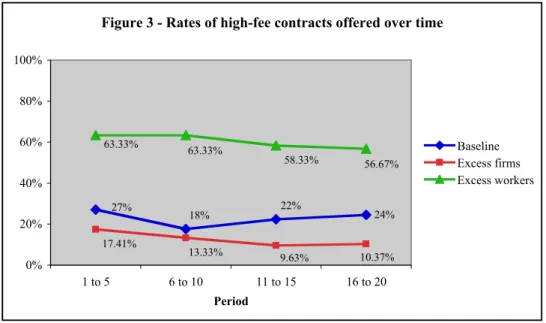
We also consider whether firms change their choice of contract over time. Figure 3 shows the rate of high-fee contracts offered in the second stage, by five-period blocks of time. These curves are the complement of the curves displayed in Figure 1. For example, the

proportion of high fees in the excess-workers treatment should be related to the fact that in the last periods some workers choose to conceal their ability; however, the decline is not significant (Wilcoxon test, p > 0.100). Overall, we see very little change over time, although a Wilcoxon test indicates that the average fee is lower in the last 10 periods than in the first 10 periods of the excess-firms treatment (p = 0.026).

Figure 3 - Rates of high-fee contracts offered over time

24% 27% 18% 22% 17.41% 13.33% _{9.63% 10.37%} 63.33% _63.33% 58.33% _56.67% 0% 20% 40% 60% 80% 100% 1 to 5 6 to 10 11 to 15 16 to 20 Period Baseline Excess firms Excess workers

Table 6 presents a regression that highlights the determinants of whether a firm chooses the high rental fee in the second stage. We estimate random-effects Probit models on pooled

21 _{If the firm is certain that the worker in fact has low talent, then there are only three chances in eight that the other}

worker has high talent. In this case, assuming own-money-maximization, a contract with the high rental fee will earn an average of 24.75 for the firm; this compares with 30 with the contract with low rental fees. For the expected revenue to be the same for both contracts, the firm must expect that about 12% of the high-talent workers hide their talent in the first stage – which corresponds to the actual value.

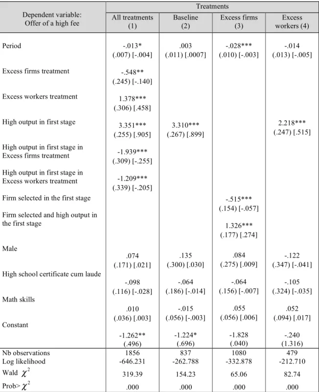
data (1) and on each treatment separately (2 to 4). The explanatory variables include the choice by the worker of a high output in the first stage. We interact this variable with each treatment in the first regression. In regression (3), we add a dummy indicating whether the firm was selected in the first stage and the same variable is interacted with the choice of a high output by the worker.

The regressions confirm the patterns we have mentioned for firms. There is no significant time trend except in the excess-firms treatment, which probably indicates the

presence of learning. Individual characteristics play no role in the firm’s behavior. Compared to the baseline treatment, firms were substantially more likely to offer a high-fee contract in the excess-workers treatment and substantially less likely to do so in the excess-firms treatment. Overall, firms were more likely to choose the high-fee contract after having observed a high output in the first stage. In the excess-firms treatment, being selected in the first stage reduces the likelihood of offering a high fee in the second stage by 5.7 percentage points but the worker being a high-talent agent instead increases the likelihood by 21.7 percentage points.

Regarding earnings, the firms naturally earn more (and the workers less) when there is competition among workers, since they are able to extract the informational rent of the workers and to select their employees. In the excess-firms treatment, firms earn almost the same profit as in the baseline because even though they are able to extract the informational rent of the agents, the workers can select the firms for which they are willing to work.22

22 _{The average earning for all firms is 47.11 in the baseline, 22.62 with excess firms, and 51.21 with excess workers}

(the corresponding numbers if we consider only matched firms are 47.11, 45.41, and 62.41). The average earning for all high-talent workers is 80.16 in the baseline, 103.80 with excess firms, and 43.66 with excess workers (the corresponding numbers if we consider only matched high-talent workers are 80.16, 103.80, and 70.46).

Table 6 - Determinants of a firm choosing the high rental fee in the second stage

Treatments Dependent variable:

Offer of a high fee All treatments ₍₁₎ Baseline ₍₂₎ Excess firms _{(3) workers (4)} Excess Period

Excess firms treatment Excess workers treatment High output in first stage High output in first stage in Excess firms treatment High output in first stage in Excess workers treatment Firm selected in the first stage Firm selected and high output in the first stage

Male

High school certificate cum laude Math skills Constant -.013* (.007) [-.004] -.548** (.245) [-.140] 1.378*** (.306) [.458] 3.351*** (.255) [.905] -1.939*** (.309) [-.255] -1.209*** (.339) [-.205] .074 (.171) [.021] -.098 (.116) [-.028] .010 (.036) [.003] -1.262** (.496) .003 (.011) [.0007] 3.310*** (.267) [.899] .135 (.300) [.030] -.064 (.186) [-.014] -.015 (.056) [-.003] -1.224* (.696) -.028*** (.010) [-.003] -.515*** (.154) [-.057] 1.326*** (.177) [.274] .084 (.275) [.009] -.064 (.156) [-.007] .055 (.056) [.006] -1.828 (.040) -.014 (.013) [-.005] 2.218*** (.247) [.515] -.122 (.347) [-.041] -.105 (.324) [-.035] .052 (.094) [.017] -.240 (1.316) Nb observations Log likelihood Wald !2 Prob>!2 1856 -646.231 319.39 .000 837 -262.788 154.23 .000 1080 -332.878 65.06 .000 479 -212.710 82.74 .000 Note: Standard errors are in parentheses and marginal effects are in brackets.

5. Conclusion

We study the ratchet effect in a simple, context-rich experimental environment. In our baseline treatment, which—like the existing experimental studies—does not incorporate ex post competition for agents or principals, we find strong evidence of the early pooling equilibria predicted by the basic ratchet model. This contrasts with the existing experimental studies, where the ratchet effect was either absent or took considerable time to develop. Since our subjects are inexperienced college students, this suggests that the ratchet phenomenon can readily emerge in real-world situations where the agents presumably have more experience and more time to ponder their actions. Especially in situations where there is a high probability of future interaction between ‘incumbent’ principals and agents, and where market alternatives for both agents and principals are scarce or unattractive, principals are wise to consider possible ratchet effects when structuring contractual arrangements.

That said, we also find that the ratchet effect essentially disappears when we introduce ex

post competition for either agents or principals. While Kanemoto and MacLeod (1992)

predicted this in the case of competition between principals, to our knowledge no studies have predicted or tested this effect of ex post competition between agents. When principals compete, we find that able agents no longer attempt to conceal their ability at the beginning of the

principal-agent relationship, since agents anticipate that the principals will not be able to extract informational rents in the future. When agents compete, they are willing to signal their ability early in the relationship in order to secure a scarce match in the future. Thus the informational asymmetry again vanishes, but in this case principals are in a position to extract all the agents’ informational rents ex post.

Taken together, our results regarding the effects of competition may have significant implications in the many domains where the ratchet effect has been studied theoretically. For example, increased competition in previously centrally-planned economies should contribute to an increase in efficiency, not only for the reasons that are most commonly discussed, but also due to a reduction in the deleterious effects of informational asymmetries between firms and their customers (formerly the central planner). In the domain of regulation, the addition of additional possible customers for utilities after efficiency-improving investments have been made should reduce utilities’ tendency to under-invest in those improvements, as will

competition among utilities for the chance to serve a common customer. Concerning optimal income taxation, the option to move between tax jurisdictions (whether states or countries) should raise workers’ effort (and improve social welfare) for reasons that are distinct from the usual work-disincentive effects of taxation;23 competition among workers for the right to remain matched with a jurisdiction (for example among recent immigrants) should also raise their effort but with a first-round effect of lower worker utility. And of course, competition between corrupt officials should reduce their ability to extract rents from customers,24 _{and competition among}

potential customers—while benefiting corrupt officials—should also reduce informational asymmetries by encouraging customers to reveal their willingness to pay up front. In sum, the ratchet effect is highly vulnerable to ex post competition on both sides of the market. This is a beneficial effect of market competition that has not been widely appreciated to date, and that is distinct from the usual arguments made in competition’s favor.

23 _{Bucovetsky (2003) has recently argued that that inter-jurisdictional worker mobility imposes efficiency-improving}

constraints on tax authorities in the context of the ‘brain drain’. The mechanism, however, is related to holdup problems associated with educational investments, which are quite distinct from the informational asymmetries modeled here.

24 _{Note that this effect is distinct from the possible advantages of rotating officials to minimize repeat interactions}

References

Allen, Douglas W. and Dean Lueck (1999), “Searching for Ratchet Effects in Agricultural Contracts” Journal of Agricultural and Resource Economics 24(2) (December): 536-52. Bucovetsky, S. (2003), “Efficient Migration and Income Tax Competition” Journal of Public

Economic Theory, 5(2): 249-78

Cabrales, Antonio, Gary Charness and Marie Claire Villeval (2006), “Competition, Hidden Information and Efficiency: An Experiment” IZA Discussion Paper 2296, Bonn. Chaudhuri, Ananish (1998), “The ratchet principle in a principal agent game with unknown

costs: an experimental analysis” Journal of Economic Behavior and Organization 37, 291-304.

Choi, Jay-Pil and Marcel Thum (2003), “The Dynamics of Corruption with the Ratchet Effect”

Journal of Public Economics 87(3-4)(March): 427-43

Brandts, Jordi and Gary Charness (2004), “Do Labour Market Conditions Affect Gift Exchange? Some Experimental Evidence,” Economic Journal 114, 684-708.

Cooper, David J., John H. Kagel, Wei Lo and Qing Liang Gu (1999), “Gaming Against

Managers in Incentive Systems: Experimental Results with Chinese Students and Chinese Managers” American Economic Review 89(4), (Sept), 781-804.

Dalen, Dag-Morten (1995), “Efficiency-Improving Investment and the Ratchet Effect” European

Economic Review 39(8) (October) 1511-22.

Dearden, James; Ickes, Barry W; and Larry Samuelson (1990), “To Innovate or Not to Innovate: Incentives and Innovation in Hierarchies” American Economic Review 80(5) (December): 1105-24

Dewatripont, Mathias, Ian Jewitt, and Jean Tirole (1999), “The Economics of Career Concerns, Part 1: Comparing Information Structures” Review of Economic Studies 66(1) (January): 183-198.

Dillen, Mats and Michael Lundholm (1996), “Dynamic Income Taxation, Redistribution, and the Ratchet Effect” Journal of Public Economics 59(1) (January): pp. 69-93.

Gibbons, Robert, “Piece-Rate Incentive Schemes” Journal of Labor Economics 5 (October 1987): 413-29.

Ickes, Barry W. and Larry Samuelson (1987), “Job Transfers and Incentives in Complex Organizations: Thwarting the Ratchet Effect” RAND Journal of Economics 18(2) (Summer): 275-86

Laffont, Jean-Jacques, and Jean Tirole (1988), “The Dynamics of Incentive Contracts”

Econometrica, 56, 1153-75.

Laffont, Jean-Jacques, and Jean Tirole. “A Theory of Incentives in Procurement and Regulation”. Cambridge, MIT Press, 1993.

Lazear, Edward (1998), Personnel Economics for Managers. New York: Wiley.

Kanemoto, Yoshitsugu and W. Bentley MacLeod (1992), “The Ratchet Effect and the Market for Secondhand Workers” Journal of Labor Economics 10(1) (January), 85-98.

Mathewson, Stanley B. (1931), Restriction of Output among Unorganized Workers, New York, Viking Press.

Puller, Steven L. (2006), “The Strategic Use of Innovation to Influence Regulatory Standards”

Journal of Environmental Economics and Management 52(3) (November), 690-706.

Roland, Gerard, and Khalid Sekkat (2000), “Managerial Career Concerns, Privatization and Restructuring in Transition Economies” European Economic Review 44(10) (December), 1857-72.

Weitzman, Martin L. (1980) “The ‘Ratchet Principle’ and Performance Incentives” Bell Journal

of Economics 11(1) (Spring), 302-08.

Appendix A – Instructions of the excess-firms treatment (other instructions available upon

request)

We thank you for participating in an experiment on decision-making. During this session, you can earn money. The amount of your earnings depends on your decisions and on the decisions of the other participants in this session. During the session, your earnings will be calculated in Experimental Currency Units, with:

100 ECU= 1 Euro.

The session consists of two parts, each including several periods. The earnings you have made during these 2 parts will be added up and converted into Euros. In addition, you will receive € 5 for participating in the experiment. Your earnings will be paid to you in cash in private.

Your decisions are anonymous and confidential.

There are three categories of players: firms, low-productivity workers and high-productivity workers. The number of firms is twice the number of workers. The high-productivity workers represent one third of the total number of workers. For example, as in this session, 18 participants are firms, 6 participants are low-productivity workers and 3 participants are high-productivity workers. The low-high-productivity workers are not human-subjects but computer-subjects.

During each period of each part, two firms are matched with one worker randomly chosen. Firms do not know the productivity of this worker. The chances are one in three (33%) that they are matched with a high productivity (human worker). The chances are two in three (67%) that the firms are matched with a low-productivity computer-worker. At each new period, firms and workers are re-matched randomly.

You are allocated either the role of a firm or the role of a high-productivity worker at random. You will be informed of your role at the beginning of the first part and you will keep the same role throughout the session.

You have received the instructions for the first part of the session. The instructions for the second part will be distributed after the first part has been completed.

The first part consists of 5 periods.

First part - Description of each period

Each of the two firms is the owner of a food concession stand on a University campus. They are willing to rent their stands to the worker for one week. The two firms charge a rental fee of ECU 15 to use the stand. This rental fee is the only source of earnings of the firms. The worker can accept at most one offer.

- If the worker rejects both offers, the firms and the worker earn 0 ECU.

- If the worker accepts one offer and rents a stand, he or she buys all his supplies for the week and keeps all the proceeds from sales.

The worker who rents the stand chooses to deliver either a low output (i.e. serving a low number of customers) or a high output in the week (i.e. serving a high number of customers).

As mentioned earlier, the low-productivity workers are computers in this experiment. They always accept one of the two 15-ECU offers at random and they choose the low output. Therefore, the firm who rents the stand to a low-productivity computer-worker earns automatically ECU 15 and the other firm earns 0 ECU.

A high-productivity worker earns ECU 22.5 net if he or she chooses the low output and he or she earns ECU 35 net if he or she produces the high output. In both cases, the firm who rents the stand to a high-productivity worker earns ECU 15 and the other firm earns 0 ECU.

The net payoffs in ECU (i.e. after payment of the rent and supplies) associated with each possible decision of the participants are summarized in the following Table:

High-productivity

worker’s choice Firm’s payoff High-productivity worker’s payoffs

Rejects the offer 0 0

Low output 15 22.5 High output 15 35 Low-productivity worker’s choice (*) Firm’s payoff Low output 15

(*) A low-productivity computer-worker always accepts the offer and always chooses the low

output.

The timing of decisions is the following:

- The two firms offer to their worker to rent the stand for ECU 15. The worker receives both offers at the same time.

- If the worker is a low-productivity worker (i.e. a computer-worker), it accepts the offer of one firm chosen randomly and it chooses the low output.

- If the worker is a high-productivity worker, he or she chooses between accepting one of the two offers and rejecting both offers. If he or she accepts one of the two offers, he or she chooses between the low and the high output.

- The firm who has been chosen is informed of these choices but he or she is not informed of whether she was matched with a high-productivity worker or with a computer-worker. The other firm is only informed that his or her offer has not been accepted.

- One’s own payoff is displayed and the period ends.

At the end of a period, a new period starts automatically. Each period is independent. Firms and workers are re-matched at the beginning of each new period.

---

Throughout the entire session, direct communication between participants is strictly forbidden. If you have any question regarding these instructions, please raise your hand. Your questions will be immediately answered in private. Please answer the comprehension questionnaire that will be displayed on your screen.

(Instructions distributed after the first part has been completed) The second part consists of 20 periods.

Each period now consists of two stages. These two stages represent the first week (Stage 1) and the next two weeks (Stage 2), respectively.

You keep the same role as in the first part.

Two firms are matched with the same worker, randomly chosen, during the two stages of one period. At each new period, firms and workers are re-matched randomly.

Stage 1

The rules for Stage 1 are exactly the same as for Part 1.

Each of the two firms proposes to rent his or her food concession stand in the first week. The firms charge a rental fee of ECU 15. This rental fee is the only source of earnings of the firms. The worker can accept at most one offer.

- If the worker rejects both offers, the firms and the worker earn 0 ECU in this stage.

- If the worker accepts one of the two offers, he or she chooses to deliver either a low output or a high output in the week.

As before, the low-productivity workers are computers. They always accept one of the offers and they choose the low output. The firm who is chosen earns ECU 15 and the other one earns 0 ECU.

A high-productivity worker earns ECU 22.5 net if he or she chooses the low output and ECU 35 net if he or she chooses the high output. In both cases the firm who is chosen earns ECU 15 and the other firm earns 0.

The net payoffs in ECU in the first stage associated with each possible decision of the participants are summarized in the following Table:

High-productivity

worker’s choice Firm’s payoff High-productivity worker’s payoffs

Rejects the offer 0 0

Low output 15 22.5

High output 15 35

Low-productivity

worker’s choice (*) Firm’s payoff

Low output 15

(*) A low-productivity computer-worker always accepts the offer and always chooses the low

output.

- The two firms offer to their worker to rent the stand for ECU 15.

- If the worker is a low-productivity worker (i.e. a computer-worker), it accepts the offer of one firm chosen randomly and it chooses the low output.

- If the worker is a high-productivity worker, he or she chooses between accepting one of the two offers and rejecting both offers. If he or she accepts one of the two offers, he or she chooses between the low and the high output.

- The firm who has been chosen is informed of these choices. The other firm is only informed that his or her offer has not been accepted.

- One’s own payoff in Stage 1 is displayed and Stage 1 ends.

Stage 2

For the right to use their concession stand for the next two weeks, the firms choose to charge a rental fee of either ECU 30 or ECU 66. The worker can accept at most one offer.

- If the worker rejects both offers, both firms and the worker earn 0 ECU in this stage.

- If the worker accepts one offer, he or she chooses to deliver either a low output or a high output in the next two weeks.

The low-productivity computer-workers always reject the high rental fee offer of ECU 66. They always accept the low rental fee offer of ECU 30 and choose the low output. If both firms offer the high rental fee of ECU 66, they reject both offers. Therefore, a firm who is matched with a computer-worker earns 30 if he or she chooses the low rental fee and 0 if he or she chooses the high rental fee.

The net payoffs in ECU for the next two weeks associated with each possible decision of the participants in Stage 2 if the firm charges the low rental fee (ECU 30) are summarized in the following Table:

High-productivity worker’s choice

Firm’s payoff High-productivity

worker’s payoffs

Rejects the offer 0 0

Low output 30 45 High output 30 70 Low-productivity worker’s choice (*) Firm’s payoff Low output 30

(*) A low-productivity computer-worker always accepts the offer with the low rental fee and

always chooses the low output.

The net payoffs in ECU for the next two weeks associated with each possible decision of the participants in Stage 2 if the firm charges the high rental fee (ECU 66) are summarized in the following Table:

High-productivity worker’s choice

Firm’s payoff High-productivity

worker’s payoffs

Rejects the offer 0 0

Low output 66 9

High output 66 34

Low-productivity worker’s choice (*)

Firm’s payoff

Rejects the offer 0

(*) A low-productivity computer-worker always rejects the offer with the high rental fee. The timing of decisions is the following:

- Each firm chooses between the low rental fee (ECU 30) and the high rental fee (ECU 66). The agent receives both offers at the same time.

- If the worker is a low-productivity computer-worker, it rejects both offers if both firms propose the high rental fee. It accepts one offer randomly if both firms offer the low rental fee. If only one firm offers the low rental fee, it accepts this offer and it chooses the low output.

- If the worker is a high-productivity worker, he or she chooses between accepting one of the two offers and rejecting both offers. If he or she accepts one of the two offers, he or she chooses between the low and the high output.

- The firm who has been chosen is informed of these choices. The other firm is only informed that his or her offer has not been accepted. The firms are not informed of whether they were matched with a high-productivity worker or with a computer-worker. - Own payoffs in Stage 2 and for the whole period are displayed. The payoff of the period

is the sum of the payoffs of each stage.

At the end of a period, a new period starts automatically. Each period is independent. Firms and workers are re-matched randomly at the beginning of each new period.

---