A spectral synergy method to retrieve martian water vapor column-abundance and vertical distribution applied to Mars Express SPICAM and PFS nadir measurements

HAL Id: insu-01865343

https://hal-insu.archives-ouvertes.fr/insu-01865343

Submitted on 28 Aug 2020

HAL is a multi-disciplinary open access

archive for the deposit and dissemination of

sci-entific research documents, whether they are

pub-lished or not. The documents may come from

teaching and research institutions in France or

abroad, or from public or private research centers.

L’archive ouverte pluridisciplinaire HAL, est

destinée au dépôt et à la diffusion de documents

scientifiques de niveau recherche, publiés ou non,

émanant des établissements d’enseignement et de

recherche français ou étrangers, des laboratoires

publics ou privés.

Distributed under a Creative Commons Attribution| 4.0 International License

column-abundance and vertical distribution applied to Mars Express SPICAM and PFS nadir

mea-surements. Icarus, Elsevier, 2019, 317, pp.549-569. �10.1016/j.icarus.2018.07.022�. �insu-01865343�

Contents lists available atScienceDirect

Icarus

journal homepage:www.elsevier.com/locate/icarus

A spectral synergy method to retrieve martian water vapor

column-abundance and vertical distribution applied to Mars Express SPICAM and

PFS nadir measurements

F. Montmessin

, S. Ferron

a_{LATMOS/IPSL, UVSQ Université Paris-Saclay, UPMC University Paris 06, CNRS, Guyancourt, France} b_{ACRI-ST, boulevard des Garennes, Guyancourt, France}

A B S T R A C T

Up to now, all attempts to retrieve martian water vapor from nadir observations have focused their analysis on a single spectral domain and comparison between the results of various experiments showed the difficulty to reconcile the water vapor datasets together. Inspired by a methodology recently developed for the analysis of Earth observations, a spectral synergy approach has been tested on the water vapor extraction from the measurements of two instruments onboard Mars Express. These instruments cover near-infrared (NIR) and thermal infrared (TIR) domains within which water vapor possesses diagnostic absorption/emission signatures. Since the two instruments have operated concomitantly around Mars, co-located measurements could be selected and processed to create a dataset exploitable by synergy. The synergy relies on a Bayesian inference algorithm tofind the best fitting values of water vapor and other parameters (e.g. atmospheric and surface temperature, dust opacity) simultaneously for both NIR and TIR intervals. Results demonstrate that synergy augments the information content about water vapor by up to >50% compared to traditional non-synergistic methods. Not only does the synergy provide an unbiased estimate of the total column abundance of H2O but it

also provides a correspondingly unbiased estimate of H2O abundance in thefirst 5 km of the boundary layer, an atmospheric region long remained unexplored

although being known for hosting key mechanisms controlling the fate of volatiles on Mars. Using synergy, the scientific return of nadir observations of current and future missions at Mars (such as the ExoMars Trace Gas Orbiter) can be fully optimized.

1. Introduction

On Earth, the global mapping of trace species has been accom-plished thanks to measurements made by passive remote sensors in orbit onboard satellites (e.g. IASI, GOSAT, SCIAMACHY, etc.). In a nadir viewing geometry, these instruments are used to return a single information regarding the species: that is either the column-integrated abundances in the case of Near-Infrared measurements (NIR) or the middle atmosphere concentration in the case of Thermal Infrared measurements (TIR), leaving open the question of how these species are distributed throughout the vertical and in particular how they interact with the surface (sources and sinks). However, new methods for re-trieving trace species in a nadir looking geometry have been introduced and have shown that it is possible to extract more information from these datasets than when each dataset is analyzed separately. This is the case for CO, as described inWorden et al. (2010)who confirmed the

predictions made byPan et al. (1995,1998). In this work, the demon-stration is made that when CO is inferred from the combination of coincident TIR and NIR measurements, this opens an access to the concentration of CO in the near-surface layer, and thus brings knowl-edge about a key part of the atmosphere where this kind of gases are

emitted. Similar conclusions have been drawn for CO2 (Christi and Stephens, 2004) as well as for CH4 (Razavi et al., 2009) and O3

(Costantino et al., 2017). The reason explaining why observations of the same species in distinct wavelength intervals provide constraints on the vertical distribution is that each spectral interval provides a distinct sensitivity along the vertical. While the NIR domain is sensitive to the full column, the TIR domain is mostly sensitive to layers located in the middle atmosphere.

On Mars, all the studies conducted to date aimed at exploring the space and time variability of atmospheric species have essentially relied on a single spectral domain retrieval approach (either UV, NIR or TIR). This has been done for a number of species like H2O, CO, O3, and

aerosols (Fouchet et al., 2007; Perrier et al., 2006; Smith, 2002, 2009). Interestingly, the Mars Express (MEX) mission offers a unique oppor-tunity to test the same NIR-TIR synergistic approach as the one used for Earth's observations. In particular, there is strong interest in testing this approach to study Mars’ water vapor. Indeed, Mars possesses an active hydrological cycle characterized by significant seasonal activity of the atmospheric and surface reservoirs of water. The current properties of the martian atmosphere allow for the existence of water only in trace quantities (∼100 ppmV) and only in the solid and gaseous phases.

https://doi.org/10.1016/j.icarus.2018.07.022

Received 3 March 2018; Received in revised form 15 June 2018; Accepted 26 July 2018

⁎_{Corresponding author.}

E-mail address:franck.montmessin@latmos.ipsl.fr(F. Montmessin).

Available online 24 August 2018

0019-1035/ © 2018 The Authors. Published by Elsevier Inc. This is an open access article under the CC BY-NC-ND license (http://creativecommons.org/licenses/BY-NC-ND/4.0/).

desorption of water molecules into/from the regolith pores.

Thefirst spatial and temporal monitoring of water vapor abundance on Mars was obtained by Viking with the MAWD instrument (Mars Atmospheric Water Detector, an echelle-spectrometer which detected water vapor from the measurement of the solarflux reflected by the surface and the atmosphere around 1.38 µm, corresponding to a H2O

NIR vibrational-rotational absorption band). The MAWD climatology, covering more than one martian year (Jakosky and Farmer, 1982), made it possible to identify the northern polar ice cap as the main source of water vapor in the atmosphere of Mars when exposed to spring-summer insolation. For two decades, the MAWD data constituted the core knowledge of the water cycle, yet some intriguing features raised by these observations remained only tentatively explained, in particular the timing of release of water vapor in the atmosphere in the mid-latitudes (Jakosky, 1983; Haberle and Jakosky, 1990). In-depth analysis of this dataset has in fact highlighted the role played by the exchanges between the atmosphere and the surface. A climatology covering three martian years was then obtained by the TES (Thermal Emission Spectrometer) IR spectrometer on MGS (Mars Global Sur-veyor;Smith, 2004). TES measurement, based on the emission in the rotational band of water between 20 and 35 µm, has been considered to be more reliable than that of MAWD because of its lower sensitivity to suspended dust aerosols that were not accounted for in thefirst MAWD retrievals. However, the sensitivity of the measurement in the TIR do-main is also dependent on the thermal contrast between the atmosphere and the surface, and thus decrease in cold regions. The MEX and the MRO (Mars Reconnaissance Orbiter) missions pursued the monitoring initiated by TES in the late 90s. MEX in particular has provided water vapor retrievals from several instruments and within a variety of spectral domains: the Planetary Fourier Spectrometer (PFS) is used for its TIR retrieval capability (Fouchet et al., 2007) while its NIR channel captures water vapor at 2.6 µm (Tschimmel et al., 2008), in the same spectral interval as the one used by the Observatoire pour la Minér-alogie, l'Eau, les Glaces et l'Activité (OMEGA) hyperspectral imager (Encrenaz et al., 2005). The band at 1.38 µm, previously sampled by MAWD, is covered by SPICAM (Spectroscopy for the Investigation of the Characteristics of the Atmosphere of Mars,Fedorova et al., 2006). An important effort was conducted within the MEX community to perform a cross-comparison between all the MEX instruments capable of detecting water vapor. This cross-comparison revealed broadly dis-persed retrievals. While the trends obtained by the MEX instruments were in agreement with MAWD and TES, they also indicated a drier atmosphere around the North Pole in summer. In this region, OMEGA and SPICAM gave comparable results while at mid-latitudes, OMEGA, in agreement with MAWD, gave 1.5 times more H2O than SPICAM did.

PFS TIR channel gave intermediate results between TES and SPICAM. These discrepancies were tentatively explained by the non-uniform mixing ratio of water vapor in the troposphere (Tschimmel et al., 2008). This non-uniform distribution is actually predicted by global climate models (GCM) as inRichardson et al. (2002), Montmessin et al. (2004)

planetary boundary layer (PBL). This would address a part of the at-mosphere that is otherwise inaccessible by non-synergistic methods performed from the martian orbit and that hosts key physical processes deciding of the fate of volatiles such as water.

The present study has been guided by the following ambitions: (i) provide an evaluation of the contribution of the NIR - TIR synergy to the exploration of water vapor within the context of the MEX mission, (ii) characterize, in terms of coverage, vertical resolution, and bias, the estimators of the water vapor column obtained with a synergistic re-trieval, (iii) apply the synergistic technique to a selected set of MEX data representative of the range of variations encountered by Mars water vapor on an annual scale and at all latitudes.

Thefirst part of the manuscript (Section 2) consists in a description of the MEX mission datasets that have been employed for this study. The selection and averaging processes used for the creation of a dataset compatible with a synergistic extraction of water vapor are described. InSection 3, the forward instrumental and radiative transfer models to be inserted in the data reduction algorithm are presented with a dis-cussion on their known limitations. The Section 4is dedicated to a description of the Bayesian and the maximum likelihood formalisms chosen for the study. This section also gives a description of the two approaches (parametric and non-parametric) designed to represent water vapor vertical distribution. The results of the synergistic method are detailed inSection 5. To evaluate the additional information con-tent supplied by the spectral synergy, its results are compared to tra-ditional methods analyzing a single spectral interval at a time. Finally, a discussion regarding the whole study is conducted inSection 6, while a conclusion opening on a variety of perspectives is provided inSection 7.

2. Mars express datasets

The dataset used in this study has been assembled out of spectra acquired during Martian Year (MY) 27 by the SPICAM and PFS spec-trometers (described thereafter). It consists of an ensemble of calibrated spectra with their wavelength registration (also called Level 1, L1 products) that have beenfiltered out (seeSection 2.3). Each L1 product corresponds to a series of collocated spectra that meet a number of selection criteria made to ensure (i) sufficient quality of every in-dividual measurement, (ii) sufficient geographical and seasonal cov-erages so as to cover various dust or water ice cloud opacity config-urations, (iii) a minimum error of radiative transfer modeling due to surface inhomogeneity (in terms of albedo, emissivity or topography) within the effective field of view covered by a L1 product. While OMEGA data could have been inserted in the synergistic study, this option has been discarded considering the results of preliminary per-formance tests that did not end up in a meaningful improvement of the synergy when adding OMEGA.

2.1. The SPICAM instrument

SPICAM is a dual UV-IR spectrometer (Bertaux et al., 2006). In the context of our study, only the IR part of SPICAM is considered since it is the one that covers the H2O 1.38 µm absorption feature. A complete

description of the SPICAM infrared channel (SPICAM-IR) can be found inKorablev et al. (2006). The instantaneousfield of view (FOV) of the instrument is 1° (equivalent to a footprint of ∼4 km at MEX orbit periapsis). This characteristic, in addition to a relatively good signal to noise ratio (SNR), has proven to be adequate for H2O column

abun-dance mapping (Fedorova et al., 2006andTrokhimovskiy et al., 2015). In our analysis, we use the data from detector 1 between 1.34 and 1.43 µm (henceforth the NIR domain of our spectral synergy), which provides significantly higher performances compared to detector 2 (the SPICAM IR channel spatially separates the incomingflux into two po-larization components as a consequence of the birefringent property of the TeO2crystal located in the active filter of the instrument). The

radiometric noise is wavelength independent in this range (Korablev et al., 2006) and its absolute level is thereforefixed, as ex-plained inSection 2.3.

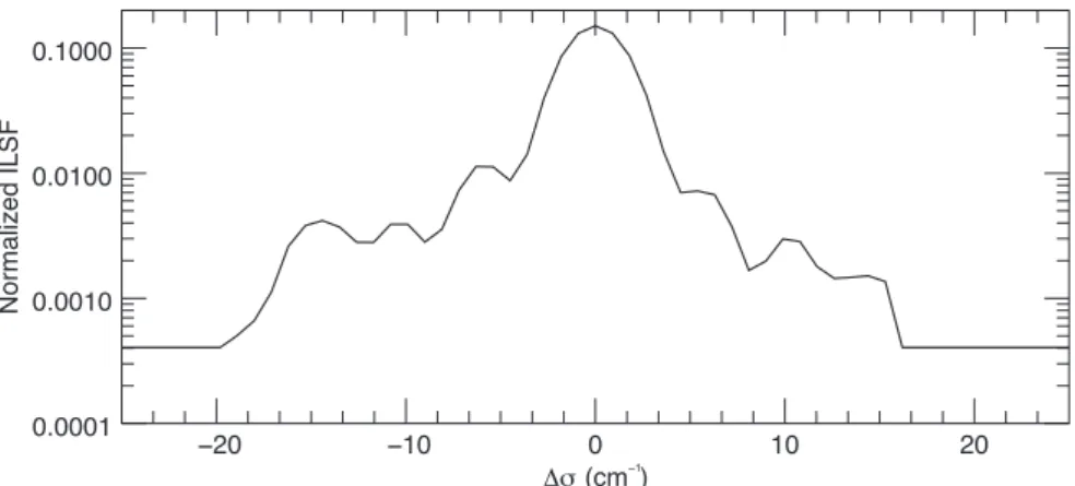
We use a wavelength dependent parameterization of the instrument line shape function (ILSF) that was supplied to us by Anna Fedorova (IKI). Stray light has a huge effect on the retrieved water vapor column abundance. Its contribution has been evaluated based on a « grey » modeling of the ILSF far wings in a similar fashion as in

Korablev et al. (2013). Details on the assessment procedure are given in S1. Thefinal ILSF is shown inFig. 1. The systematic error associated with the uncertainty of the stray light contribution is around∼10%, that is of the order of the statistical error.

2.2. The PFS instrument

A detailed description of the PFS (Planetary Fourier Spectrometer) Fourier transform spectrometer can be found in

Formisano et al. (2005), only the most relevant characteristics are listed here. The full width at half maximum (FWHM) of the instantaneous FOV of the instrument is equal to 2.7°, corresponding to a 12 km-dia-meter footprint at periapsis. The unapodized spectral resolution is roughly 1.3 cm−1. We use a sine cardinal parametrization of the in-strument transfer function whose FWHM is adjusted from the data as explained in S2; together with a wavelength assignment parameter.

In this analysis, several overlapping spectral windows have been defined in the TIR domain. The TIR2 band extends from 20 to 35 µm and is used to retrieve the water vapor abundance. However, retrieving H2O in the TIR domain requires a good and independent knowledge of

the atmospheric temperature profile. To this end, we have considered the TIR1 band between 12 and 19 µm, which is characterized by the strong absorption of the CO215 µm vibrational transition. A third

do-main, TIR3, has been defined to constrain the surface temperature and

the dust model properties. It spans the regions between 8 and 10 µm µm and between 19 and 25 µm.

The TIR2 band has been used to map the water vapor column abundance in Fouchet et al. (2007). As explained in this paper, the signal-to-noise ratio (SNR) of a single spectrum is not high enough to infer a reliable value for the column abundance. Replicating what was done is Fouchet's study, we average 9 consecutive spectra upon which a retrieval of the water vapor is performed. Other parameters (i.e. tem-perature and dust optical depth) are retrieved this way as well whereas

Fouchet et al. (2007)performed a temperature retrieval of individual spectrum. Furthermore, in order to reduce the influence of errors arising from inter and/or intra FOV observation conditions hetero-geneities that are not represented in our modeling, we apply a set of selection rules namely: (i) the effective FOV corresponding to the 9 averaged spectra must span a distance less than 300 km on the martian geoid (that is 5° for a geoid radius of 3396 km), (ii) the airmass factor corresponding for each individual spectrum varies by less than 1%, (iii) the variation of topography within the 9 instantaneous FOV and be-tween them is less than 1% of the mean scale height of the atmosphere (∼0.1 km), (iv) the variation of the TES albedo (cf.Section 3.4) within the effective FOV is less than 3%, (v) at least one observation of SPICAM-IR lies within the effective FOV of PFS, (vi) no overlap occurs between effective FOV.

2.3. Synergy level 1

2.3.1. SYN spectra

The synergy method requiresfirst to assemble a set of combined NIR and TIR spectra (SYN product) upon which the retrieval algorithm is applied. In order to ensure a common horizontal spatial resolution between NIR and TIR measurements, all SPICAM-IR spectra with a FOV inside the effective FOV of the SYN product (corresponding to 9 PFS FOV, cf.Section 2.2) are averaged together. An additional screening is performed that performs selection based on the following considera-tions: (i) the NIR airmass factor corresponding to an individual spec-trum varies by less than 1%, (ii) the selected spectra are contiguous, (iii) the relative variation of the albedo in the NIR band stays within a 5σ dispersion of the radiometric noise (to do so, the albedo is estimated with a polynomialfit of the smoothed spectra).

Thefinal dataset comprises 449 SYN spectra distributed among 133 orbits encompassing the entire MY27.

2.3.2. Noise consideration

The overall mean SNR for each channel is displayed inFig. 2. In the TIR, the radiometric noise is obtained by smoothing the wavenumber dependent radiometric variance curve calculated from the 9 spectra. In the TIR1 band (temperature) the mean SNR lies typically between 70 and 140. In the TIR2 band (water vapor), SNR values vary between 90 and 220.

Inside a SYN spectrum, 10–20 individual SPICAM-IR spectra are typically averaged together. A variance analysis in the continuum range is used to determine the level of radiometric noise of the SPICAM-IR data (it is found to be roughly 60% of the noise value given in

Korablev et al. 2006). For an individual spectrum, the SNR lies typically between 130 and 240. For an average spectrum, a covariance ac-counting for the FOV to FOV albedo variability is added to the radio-metric covariance. This accounts for the too permissive 5σ selection rule stated above and contributes to the high variability of the SNR. A comparison between water vapor column abundances inferred from individual SPICAM-IR spectra and the column abundances inferred from a SYN spectrum at its effective FOV is presented in S3. The ob-servedfluctuations have a magnitude of the order of the estimated er-rors and a non-zero mean value.

It is to be noted that the selection method was deliberately re-strictive to maximize the chances of drawing benefits from the synergy in the retrievals and to ensure synergy would not be evaluated against a biased orflawed dataset. Working with the best cases does not grant a universal application of the method but at least its potential can be established in a sound manner. In a subsequent part of the study, one might be interested to optimize the selection criteria so as to maximize the number of observations retained for the retrieval and thereby reach and extract the full“breadth” of the Mars Express dataset in the context of synergy. According to our preliminary evaluation, the Mars Express synergistic dataset potentially contains up to 200 000 co-located spectra matching the selection criteria, to be compared with the 449 selected and presented here.

2.4. OMEGA data

We did not use the OMEGA (Observatoire pour la Minéralogie, l'Eau, les Glaces et L’ Activité) measurements at 2.56 µm because, as shown by a previous investigation based on synthetic simulated data, the information provided by the OMEGA and SPICAM spectrometers on the vertical distribution of water vapor are qualitatively redundant (in terms of degrees of freedom for the signal, DOFFS, and vertical cov-erage). Besides, the performances of OMEGA for retrieving water vapor are slightly degraded compared to SPICAM due to its lower spectral resolution. Indeed, at OMEGA spectral resolution, the 2.6 µm band of water vapor is more complex to analyze due to the nearby presence of a deep CO2absorption feature that is merged with that of H2O vapor. As a

consequence, no significant influence of the OMEGA data is expected to exist on the synergistic retrieval when SPICAM-IR data are used.

3. Forward model

A complete forward radiative transfer model was developed to re-produce the type of observations performed by the MEX instruments considered in this study. In that context, one has to account for a variety of processes involved in the radiative transfer configuration of each wavelength interval to be analyzed (the NIR, TIR1, TIR2 and TIR3 bands). This forward model is eventually inserted in the middle of the spectral inversion loop so as to perform the parameter adjustment, in-cluding those related to water vapor.

3.1. Molecular absorption

The HITRAN 2012 (Rothman et al., 2013) spectroscopic database is used as a baseline to compute the absorption coefficient by CO2and

H2O. CO2 lines shape parameters come from precise measurements

and/or from theoretical or semi-empirical predictions. When sources are available, they are in good agreement and the experimental in-formation is supplied by HITRAN.

3.1.1. Spectroscopic parameters

The collisional widths of H2O lines have to be corrected to take into

account the CO2atmosphere of Mars. In the NIR domain, multiplying

the foreign collisional width parameters by a factor of 1.6 accounts for this. The sensitivity of the water vapor column retrieval to this para-meter is investigated in S4. In the TIR domain, we rely on the calcu-lations ofBrown et al. (2007), which provide a modified value of the

half width, its temperature dependence, and the pressure-shift para-meters.

In the NIR spectral range, most of the molecular absorption is due to the H2O vibrational band centered at 1.38 µm (the absorption by CO2is

negligible). The interval between 1.4 and 1.42 µm is characterized by a low absorption of H2O. This interval could help disentangle the aerosols

and surface contribution to the continuum, which is an important issue since dust aerosols modulate the optical path length of photons and have therefore an impact on the retrieved water vapor content. However, the NIR domain does not allow for an unambiguous de-termination between dust optical depth and the water vapor column and a dust model has to be derived elsewhere.

3.1.2. Line mixing

In the TIR1 and TIR2 ranges, the emission is due respectively to the 15 µm vibrational band of CO2 and to the rotational band of H2O

ranging from 20 and 40 µm. The line-mixing effect in the CO215 µm

vibrational transition region leads to a slight decrease of the absorption coefficient in the far wings of the band (based on a calculation by

Niro et al., 2004). Although it may have an impact on the derivation of the temperature profile, we decided to neglect it to limit the absorption coefficient calculation time. In the TIR3 band, the residual absorption by CO2between 9 and 11 µm (seeFig. 1ofSmith, 2004) is neglected

and the H2O contribution between 19 and 25 µm is removed using a low

passfilter as explained inSection 4.1. 3.1.3. Isotope line intensities

In HITRAN, the line intensities are weighted by the Earth relative isotopic abundances, but no adaptation to the martian configuration exists. Partition function at local thermodynamic equilibrium is com-puted with the total internal partition sums (TIPS) program of

Laraia et al. (2011). A parallelized version of a code (Wells, 1999) that implements the Humlicek algorithm (Humlícek, 1982) is used to cal-culate the Voigt line shape at all atmospheric levels. The thresholding technique described inLetchworth et al. (2007)is implemented in order tofilter out lines with small intensities and save computation time. We have checked that the absorption coefficients obtained in this way were in good agreement with those obtained with the well-validated code LBLRTM (Clough et al., 1992,1995).

3.1.4. Absorption cross-section determination

We rely on the correlated-k approximation (Fu et al., 1992) to in-crease the speed of radiative transfer calculations. The correlated k-distributions (CKD) are defined by a Gauss-Legendre quadrature with 16 nodes on spectral intervals whose extents correspond to a fraction of the ILSF's FWHM (namely 0.9 and 0.4 cm−1 respectively for the SPICAM and PFS). The CKD are tabulated as a function of the tem-perature (between 70 and 350 K by step of 10 K), pressure (5 points per decade between 10−2and 10 hPa) and (for NIR and TIR2 only) water vapor volume mixing ratio (58 points, regularly spaced on a log-scale between 10−7 and 4 × 10−2). The « kdistribution_light » package (Eymet, 2014) has been used to compute the CKD lookup tables (LUT).

3.2. Scattering by aerosols

In this study, scattering by water ice clouds has not been considered due to the small impact on the retrieved water vapor parameters as deduced from the tests performed with, a selected set of samples (see S6 for additional details). To describe the extinction by dust, we rely on an inherent optical properties (IOP) database provided to us by Wolff (Clancy et al., 2003; Wolff et al., 2003,2009). Starting from a set of experimental constraints on microphysical properties (complex refrac-tion index, particle size) the absorprefrac-tion and angular scattering cross-section have been calculated, between 260 nm and 50 µm, using the Mie theory. In the database, the angular dependence of the scattering phase function is represented by its asymmetry parameter g. Seven models are available. They correspond to lognormal particle size dis-tribution (dispersion: 0.3 µm) with an effective radius ranging from 0.1 and 3 µm for lognormal particle size distribution. The scattering is negligible in the TIR channels as a result of the low single scattering albedo of dust (SSA) in TIR2, TIR3 and TIR2 (this channel being dominated by the strong CO2ν2band). This is illustrated inSection 5.1.

In the NIR domain, the IOP are rather independent of the wave-length. For small particle size (radius <0.1 µm) the asymmetry para-meter is close to 0.2 while for a coarser particle it is equal to roughly 0.7. Considering these values, the Henley-Greenstein function can be used within a good approximation to represent the scattering phase function. Our scattering model relies on the discrete ordinate method to solve the radiative transfer equation (RTE) (see Section 3.5). In this approach, the scattering phase function is described by Legendre polynomials whose truncation is chosen in accordance to the value of g. The Delta-M approach is used to reduce the dependence of the precision

of the calculations to the number of polynomial coefficients in case of a g value close to 1.

The vertical distribution of dust is described by the volume mixing ratio (vmr) profile predicted by the Mars climate database (MCD). Microphysical properties of dust are assumed independent of altitude. The dust absorption band in the TIR3 domain is used to define both the dust optical depth (DOD) at 9 µm and the best set of IOP (that is the best effective radius). We have assumed that the representation of dust in the MCD is sufficiently realistic to establish a correlation between the DOD predicted by the MCD and the DOD retrieved from the PFS data (seeSections 4.1and5.1for details).

3.3. The solar source function

Two TOA solar irradiance model have been used for the modeling of the NIR spectra: (i) a high spectral resolution (with a resolving power of 500 000) synthetic spectrum calculated in the wavelength range from 150 nm to 0.3 cm with the ATLAS12 model by Kurucz (http://kurucz. harvard.edu/stars/sun), (ii) an experimental calibrated spectrum ran-ging from 1.2 and 5 µm with a spectral resolution of∼1 nm prepared for the exploitation of the PFS data by Fiorenza et al. (2005). This spectrum is derived from several sources: between 2 and 5 µm, the space based measurements from the ATMOS experiment were used while in the range 1.2–2 µm, which includes the NIR domain, ground based measurements from the Kitt Peak observatory have been used. Both parts of the spectrum have been cross-calibrated using the solar continuum calculated by Kurucz. These spectra have been averaged over the spectral intervals used to define the CKD and have been nor-malized according to the Sun-Mars distance.

In our study, the « PFS » spectrum is taken as the reference model. It gives slightly better fit and the impact on the retrieved water vapor column abundances is negligible compared to other sources of un-certainty (see S5 for details).

3.4. Surface properties

Surface properties are considered both at data selection (through FOV uniformity conditions, seeSection 1) and during retrieval stages. The surface visible albedo and thermal emissivity have been established from TES observations (Bandfield et al., 2003; Christensen et al., 2001). Owing to its multi angular capabilities, spectral signatures associated to scattering in the atmosphere and to the surface reflection/emissions could be disentangled. Fig. 3 shows the TES surface emissivity for bright and dark surfaces as explained in Bandfield et al. (2003). A smoothing procedure has been applied in order to remove noise andfill the gap corresponding to the 15 µm CO2band that is totally absorbed.

This defines the first guess emissivity used in the subsequent TIR modeling assuming isotropic emission from the surface.

In the NIR, the value of the continuum depends on the way the atmospheric scattering is handled. Ourfirst guess albedo is defined through afirst-degree polynomial fit of the low-pass filtered spectra. The forward model assumes a lambertian behavior of the reflection distribution function of the surface. In both cases (NIR and TIR) the non-parametric Bayesian approach explained inSection 4allows for a flexible low frequency shape modulation of the continuum assuming prior auto-correlation functions.

3.5. Calculation of upwelling TOA radiances

The TOA radiance for a plane paralleled non-diffusing atmosphere is:

∫

with λ the considered wavelength. A, ɛ, TS are the surface albedo,

emissivity and temperature respectively, B the black-body emission, F the solar radiance. The integrated opacity of the layer located be-tween altitude z and TOA is given by:

∫

k(z,σ) is the total extinction coefficient corresponding to absorption by molecules and aerosols and scattering by aerosols. The molecular contributions are obtained by a tri-linear interpolation of the tem-perature, log-pressure and water vapor vmr space of the CKD nodes (see

Section 3.1). The intra-layer vertical integration ofEq. (2)is done as-suming a linear variation of the absorption coefficient with the altitude. The air density profile is computed for hydrostatic equilibrium from the high spatially resolved MOLA (Mars Orbiter Laser Altimeter) surface pressure map (accessed through the MCD) and the temperature vertical profile (taken from the MCD or estimated from the PFS-LW data).

To take into account the scattering, the single scattering albedo and scattering phase function of the atmospheric layers have to be defined as well. This is done using the Wolff database presented inSection 3.2

assuming a Legendre polynomial development of the Henley-Greenstein phase function. We use 30 terms with a number of half-space streams of 8.

The calculations of intensity taking into account the scattering rely on the LIDORT (LInearized pseudo-spherical scalar Discrete Ordinate Radiative Transfer model) RTE solver (Spurr, 2008). This model is based on a linearized formulation of the DISORT discrete ordinate ap-proach (Stamnes et al., 1988) allowing for fast analytical determination of the radiance derivatives with the atmospheric layer's IOP and surface properties (i.e. lambertian albedo and emissivity). The derivatives of the layers IOP with temperature (respectively water vapor vmr) are obtained by symmetric finite difference with a 1% perturbation (re-spectively 50%). The derivatives of the radiance with respect to the other parameters are calculated by symmetricfinite difference as well. The perturbation depends on the parameters: 1% for the stray light contribution to the SPICAM-IR's ILSF, 5% for the wavelength assign-ment shift of the PSF-LW spectra, 110% for the ILSF's FWHM of this instrument, 5% for the H2O vmr at the surface in the parametric

for-mulation discussed below and 100 m for the saturation level altitude.

4. Inversion technique

In this study, we have to consider the retrieval of a variety of quantities, some regarding instrument properties (stray light contribu-tion in SPICAM-IR, the FWHM of the ILSF and the spectral assignment for PFS) while other relate to geophysical parameters (surface albedo/ emissivity, atmospheric temperature, water vapor content and dust properties). To achieve this, three steps are followed in the estimation process:first, the instrumental parameters are determined, second the parameters of the dust model, andfinally the parameters related to water vapor, atmospheric temperature and continuum. Thefirst stage has been discussed inSection 1. The two others are discussed below.

4.1. Retrieval of surface temperature and dust properties

Scattering by aerosols may have a significant impact on the H2O

retrieval from NIR data (Trokhimovskiy et al., 2015and in S6). How-ever, the distinction between spectral signatures associated to the scattering and to the surface reflexion is difficult to achieve and may result in large uncertainties on the DOD and column abundance. For this reason, the aerosol model has to be defined prior to the H2O

re-trieval. SYN spectra in the TIR3 channel are used to retrieve i) the surface temperature, ii) the DOD at 9 µm assuming a wavelength-de-pendent IOP model taken from (Wolff et al., seeSection 3.2) and iii) the “best” dust effective radius which controls the spectral dependence of aerosols.

Between 20 and 25 µm, spectral samples contaminated by water vapor absorption are rejected: a 1-σ threshold is applied to the differ-ence between the considered spectrum and the same spectrum with a low-passfilter. In that spectral region, the dust SSA is lower than 0.2 and the extinction by water ice cloud is negligible. The second part of the TIR bands used in this analysis extends from 8.5 to 10.5 µm. It is characterized by a strong silicate absorption band of dust (SSA < 0.5). The region between 10.5 and 12.5 µm is excluded because it might be contaminated by water ice cloud extinction (seeFig. 1ofSmith, 2004). Finally, the small absorption by CO2between 9 and 9.5 µm is neglected.

The retrieval relies on a non-linear least squarefitting Levenberg-Marquardt algorithm (as implemented in the IDL package“MPFIT”,

Markwardt, 2009) using the atmospheric temperature predicted by the MCD and the TES model emissivity (Section 3.4). A lognormal variable substitution is used to force the retrieved DOD positivity. A low (0.01) value of the DOD is assumed asfirst guess. The surface temperature is defined with a first guess corresponding to the average brightness temperature between 12.1 and 12.5 µm.

The information content of the TIR domain is not sufficient to

Fig. 3. Left: dark/bright region mask built from the TES albedo map. High albedo (>0.18) regions appear in white, low albedo in black. Right: the symbols display the spectral emissivity for dark and bright regions obtained from TES data. The lines show the interpolations used in the forward model.

constrain the microphysical properties of the aerosols. So, we use the MCD to select the best model within the Wolff database. Note that our fast-radiative transfer model neglects scattering. For each radius, a full retrieval is performed that includes dust opacity as a free parameter. The retained radius is the one providing the opacity value closest to that proposed by the MCD. MCD is just used as a criterion for selection, opacity being otherwise free to vary. Results are presented in

Section 5.1.

4.2. Retrieval of temperature and water vapor content

The retrieval of the temperature and water vapor relies on the Bayesian formalism described inRodgers (2000). We assume that data is linked to the forward model through the following relation:

= +

d g m( ) ϵ (3)

whereϵis an unbiased gaussian random variable representing the noise on the measurement vector d and m correspond to the true value of the state vectors. The estimationm∼is defined by the value of m which minimizes the quadratic cost function:

= − − − + − − −

C m( ) [d g m( )]TC [d g m( )] [m m] C [m m]

d1 0T 01 0 (4)

Thefirst term corresponds to the maximum likelihood probability distribution. The second term defines the uncertainty associated to the prior m0. Since g is a non-linear function, the estimator can be

com-puted via an iterative Raphson–Newton descent method:

= + + − + −

∼ ∼ ∼

+ −

mi 1 m0 C G0 iT(G C Gi 0 iT Cd) [1d g m( i) G mi( i m0)] (5) with Githe Jacobian matrix of g m(∼i)evaluated at iteration i. In this

expression, the inversion is done (by Cholesky decomposition) in the data space, which has in our case, a smaller size than the parameter space (due to continuum parameters). The convergence criterion is based on successive variations of the normalizedχ2:

= − − ∼ − ∼ χ d g m C d g m n [ ( )] [ ( )] i i T d i d 2 1 (6) where ndis the number of data. The covariance error on∼mis given by:

= −

Cm (1 MRM C) 0 (7)

with MRM the averaging kernel (matrix resolution model):

= + −

MRM C GT(GC GT C) G

d

0 0 1 (8)

computed at convergence. The trace of MRM defines the DOFFS which corresponds to the number of independent parameters which can be constrained by data considering an a priori knowledge (m0, C0).

InEq. (4)the matrix inversion is regularized by the C0matrix. For

continuum (that is surface albedo and/or emissivity) parameters, which depend on the wavelength, C0is defined by an exponential kernel with

a sufficiently high correlation length so that only low frequency mod-ulation of the prior is retained by the estimation. Gaussian kernels are used for atmospheric profile parameters (that is water vapor vmr fluctuations relative to MCD vmr and/or temperature).

Prior experiments performed on synthetic datasets indicate that the DOFFS of H2O are roughly equal to 1 when retrievals are performed on

separate spectral domains (slightly higher for NIR, slightly lower for TIR depending on geophysical conditions). This constitutes a theore-tical confirmation that one spectral domain alone is not able to supply more than one independent information regarding water vapor. This information is usually assigned to the column-integrated abundance.

With synergy, one is capable to constrain an additional information for H2O and therefore establish a two-parameter model of the water

vapor vertical distribution. In doing so, a large prior uncertainty on the column abundance can be assumed, resulting in a column estimator close to the unbiased maximum likelihood estimator (in other words, an estimation not biased by the prior information). The two-parameter model of the water vapor vmr is represented by:

= − + − − ⎡ ⎣ ⎢ − + ⎤_⎦⎥ x z x z Y z z r z Y z z r z x z z x ( ; , s) ( s) ( ) [1 ( s)] ( ( )s ) s 0 0 0 (9) which depends on the vmr at the surface, x0, and the saturation level

altitude zs. In this expression Y is the Heavyside function:

= ⎧ ⎨ ⎩ ≥ < Y u u u ( ) 1, 0 0, 0 ₍₁₀₎

and r is the saturation ratio. The saturation vapor pressure depends only on temperature. It is calculated using the Goff-Gratch formula.

The two-parameter model assumes 100% saturation above zsand a

linear variation with altitude down to the surface. Since it cannot be sampled on a discrete vertical grid, we substitute the Heaviside function by the error function:

= − + − − ⎡ ⎣ ⎢ − + ⎤_⎦⎥ x z x z z z r z z z r z x z z x ( ; , s) erf( s) ( ) [1 erf( s)] ( ( )s ) s 0 0 0 (11) with

∫

abun-dance W predicted by the MCD. The former is obtained with the vmr profile of the MCD and

∫

∫

(

)

Fig. 4shows a comparison between an original MCD profile and the

parametric model in a case where W∼ 8 pr.µm. In this approach, un-certainty on the column abundances is calculated from the covariance associated to x0and zsestimators.

A second, non-parametric, approach, has been investigated which uses the MCD predictions as prior for our Bayesian algorithm. In that case, the goal is to identify large vertical scalefluctuations compatible with the NIR + TIR DOFFS, which might be different from single-do-main DOFFS due to the complementarity of the averaging kernels be-tween NIR and TIR in most configurations (seeSection 5.3.3). We infer two estimators for H2O: (i) the column abundance from the surface up

to the TOA, and (ii) the column abundance from the surface up to 5 km,

Fig. 4. An example of H2O vmr profile from the MCD (red) compared with the

corresponding parametric model (black). Both profiles yield the same column abundance.

both are obtained by vertical integration of the retrieved concentration.

5. Results

5.1. Step1: Retrieval of surface temperature and dust properties

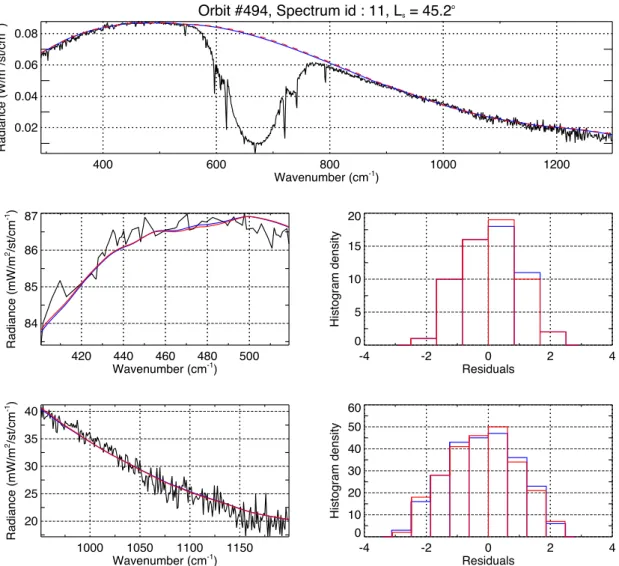
The methodology chosen to retrieve the surface temperature and dust properties from the TIR3 SYN spectra has been applied to the MY27 SYN products as previously explained. An example of forward modeling is displayed inFig. 5. Distributions of residuals are displayed separately for the two parts of the TIR3 band located on both sides of the CO2absorption band. In the shortest wavenumber region, the

ad-justed spectra have been smoothed in order to remove the main ab-sorption features while preserving the continuum shape. As illustrated in thisfigure, data are equally fitted regardless of whether scattering has been accounted for or not. The differences between the corre-sponding modeling results appear small when compared to the radio-metric noise.

An additional set of empirical criteria was established to retain only the best SYN products that will receive the complete retrieval proce-dure. The criteria are: (i) the Levenberg-Marquardt has to converge to a solution comprising a plausible DOD value and a normalizedχ2lower than 3 (seeFig. 6-left), (ii) the retrieved effective dust radius is smaller than 3 µm. The aim of the second condition is to prevent side effects resulting from the dust model selection procedure, which would

translate into a suspicious increase at the upper edge of the effective dust radius distribution (Fig. 6-middle). We see that results behave approximately like a log-normal distribution.

Finally, the retained dataset comprises 232 SYN spectra. Fig. 6

shows the correlation between the DOD obtained while taking into account or not the scattering. The exact relation between the two de-pends on the dust properties (i.e. the dust radius) and the spectral do-main used for the retrieval which controls the average value of the SSA. However, to some good approximation a linear law might be con-sidered. We note that the DOD with scattering is on average 15%−20% higher than the DOD without scattering. In the sections that follow, the DOD without scattering will be used for the TIR channels and the DOD with scattering for the NIR channel.

The estimated DOD values as well as their geographical distribution are shown onFig. 7. Zonal averaged values are presented onFig. 8. When compared with the THEMIS (THermal Emission Imaging System) climatology (Smith et al., 2009, theirFig. 6), wefind a slightly sys-tematic excess of DOD values however with the correct trends. It is to be noted that our sparse longitude sampling does not allow for an unbiased determination of zonal averages.

The correlations between our results with the predictions of the MCD are shown onFig. 9. The good correlation between the DOD is due to the retrieval approach itself since the bestfit is always leaning to-wards the MCD predictions (seeSection 4.1on the IOP model selection procedure).

Fig. 5. A typicalfit of PFS data in the TIR3 band where surface temperature and dust optical depth are is retrieved, blue: without scattering, red: full transfer with scattering. The values of the parameters are a DOD of 0.18 at 9 µm, an effective dust radius of 1.5 µm and a surface temperature of 253.2 K. The bottom plots zoom over the two edges of the TIR3 domain and display the corresponding histogram of the residuals given in %.

The DOD values obtained without scattering are found to be higher by <10% than those of the MCD, a result consistent with the outcome of our comparison with the THEMIS climatology. The cause for this small discrepancy was not searched for and it was decided instead to assign a 10% systematic uncertainty to the retrieved DOD.

5.2. Step 2: Retrieval of atmospheric temperature profiles

The retrieval of the atmospheric temperature from the TIR1 channel is based on the Bayesian formalism described in Section 4.2. The aerosol model estimated in the previous section is used and the DOD is kept constant. In that step, the retrieved parameters are the surface temperature, whosefirst guess value and its associated uncertainty are extracted from the dust retrieval (Section 5.1). The spectral emissivity of the surface is also inferred with a first guess built from the TES emissivity model (see Section 3.4). A wavelength independent prior uncertainty of 1% is applied with an exponential correlation kernel (correlation “length”: 103 cm−1). The emissivity parameter space is bounded between 0 and 1 by substitutingɛ by ≡p asin(2ɛ−1). A wa-velength shift parameter is also adjusted, taking advantage of the highly structure spectral shape of the CO215 µm band. The derivation of the

atmospheric temperature profile starts with a first guess given by the MCD. The prior covariance is defined arbitrarily, being equivalent to constant uncertainty of 30 K throughout the profile, whereas a Gaussian correlation kernel with a standard deviation of 10 km is assumed. The

FWHM of the ILSF is kept constant and is determined as explained in S1. A typical data modeling of the TIR 1 spectral interval is shown on

Fig. 10.

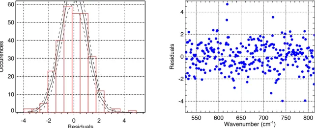
Although a goodχ2_{is achieved in this case, thefit is imperfect as}

revealed by the residual distribution displayed onFig. 11where some absorption features appear in the wings of the strong CO2 line at

16.3 µm (615 cm−1). TheFig. 12 displays the retrieval of the con-tinuum parameters. The large prior correlation“length” ensures that no steep absorption feature is assigned to emissivityfluctuation. However, the“length” is chosen small enough to tolerate moderate departure from the prior assumption. The retrieval of the atmospheric tempera-ture is shown inFig. 13. The temperature DOFFS is equal to 6.4 whereas the DOFFS for the entire retrieval is 10.8. This means that 6 to 7 in-dependent parameters can be extracted from the temperature profile, while the other 4–5 parameters pertain to surface emissivity / tem-perature as well as to the wavelength shift.

5.3. Step 3: Retrieval of water vapor

In order to gauge the potential benefit of the synergistic retrieval compared to traditional single-domain inversion techniques, the same SYN dataset was used to perform retrieval in three different manners: first, using the NIR domain only, then solely the TIR domain and finally the combination of both which establishes the synergy between the two domains.

Fig. 6. (From left to right) reducedχ2_{, number of occurrences of the dust effective radius, correlation between the DOD obtained with scattering (y-axis) and the DOD}

obtained without scattering (x-axis). Color is coded according to the effective radius value. DOD values are normalized to a reference pressure of 610 Pa.

5.3.1. NIR-only inversion

In this subsection, we analyze the results of the retrieval performed while assuming the H2O parametric vmr model ofEq. (11)and while

restricting ourselves to the NIR part of the SYN spectra. Still, we employ the aerosol model derived from the TIR3 band (seeSection 4.1) while the DOD is kept constant. In order to limit computing time, the fast-radiative transfer model presented in Eq. (1)is used. Scattering was neglected, an assumption supported by the study presented in S6.

In the“NIR only” case, the retrieved parameters are the spectral albedo of the surface whosefirst guess is built as explained in 3.4. A wavelength independent prior uncertainty of 10% is applied with an exponential correlation kernel with a“length” of 107cm−1. The posi-tivity of theses parameters is ensured by a lognormal variable sub-stitution. The other parameters are the H2O vmr at the surface, x0and

the saturation level altitude zs. Thefirst guess on these parameters are

defined based on the MCD predictions. The positivity of x0is again

ensured by a lognormal variable substitution. A 100% prior uncertainty on x0and 200 m prior uncertainty on zswere chosen. The ILSF model

presented in Section 2.1 has been used. A typical data modeling is shown onFig. 14.

An examination of the residual distributions (Fig. 15) whose fluc-tuations show distinct wavelength dependent structures suggests that a betterfit might possibly be achieved by adding a spectral shift in the state vector (as done for the PFS spectra).

The retrieval of the continuum parameters for the same SYN product is shown on Fig. 16. Since atmospheric scattering is neglected, the continuum incorporates both the surface and the atmospheric con-tributions. In this particular example, atmospheric scattering accounts for 15% of the continuum as deduced from an estimation performed with scattering. The large correlation length of the prior covariance kernel ensures that a good separation with the H2O absorption spectral

features is achieved while some continuum shape distortion is allowed. The water vapor column abundances retrieved for the entire dataset are shown in Fig. 17. The Fig. 18-left shows a comparison with

Trokhimovskiy et al. (2015). Trends are found to be in good agreement between the two despite the fact that scattering was neglected in our retrievals.

It is worth comparing retrievals based on the parametric approach to those based on the non-parametric approach (seeSection 4.2for a definition of the two models). This comparison is shown onFig. 18

-Fig. 8. Zonal averages of normalized DOD. The error bars correspond to the standard deviation within the latitude/solar longitude bin.

Fig. 9. Retrievals of DOD without scattering (left) and of the surface temperature (right) from PFS data and compared to the predictions of the MCD. Correlation coefficients (R) between PFS and MCD datasets are given in the plots.

right (see Section 5.3.3 for details on the non-parametric inversion settings). Column-integrated abundances obtained with these two ap-proaches are strongly correlated yet the parametric inversion gives roughly 10% more water vapor than the non-parametric one. Due to the small prior uncertainty assigned to the saturation level altitude, only one H2O parameter can be constrained on the vertical profile. However,

the non-parametric approach gives a DOFFS greater than 1 (that is 1.4 on average, seeFig. 25inSection 5.3.3), suggesting that the parametric model is too rigid, resulting in a systematic positive bias on the column

abundances. However, nofirm conclusion should be made out of this remark since theχ2_{improvement provided by the non-parametric}

ap-proach is low.

Here, we present the results of the H2O parametric inversion(11)

applied to the TIR spectra only. Dust scattering is treated as described in

Section 5.3.1. In addition to the parameters listed inSection 5.2 the retrieval also concerns the H2O vmr at the surface, x0and the saturation

level altitude zs, with the same inversion parameters setting as for the

NIR only case. The spectral emissivity of the surface in the TIR2 band (seeSection 5.2for the TIR1 emissivity) is also a derived product of the inversion.

Fig. 19shows an example of TIR2 spectra modeling. In general, the residuals are not evenly distributed (Fig. 20). The features that we see in the continuum parameters solution are present in the prior (built from the TES data, seeSection 3.4). As in the case of the TIR1 band (Section 5.2), the inversion parameters for emissivity ensures a good separation between absorption and surface spectral signatures.

The retrieved H2O column abundances are found to be in good

agreement with the SPICAM measurements presented in

Trokhimovskiy et al. (2015)(Fig. 21, left). Owing to the lack of sta-tistics in the latitude/solar longitude bins, it is not possible to claim a possible improvement resulting from the simultaneous temperature retrieval.

Unlike the NIR case, the inverse model formulation has little impact on the estimated H2O column abundances (given the errors bars which

are approximatively equal to 15% on average for both the parametric and the non-parametric approaches).

Fig. 10. Forward modeling of the TIR1 spectra for orbit 205, SYN spectrum #8.

Fig. 11. Residual (differences between data and model divided by the radiometric noise at 1-σ) distribution corresponding to the fit displayed inFig. 10.

Fig. 12. Retrieval of the spectral emissivity in the TIR1 band corresponding to thefit displayed inFig. 10.

5.3.3. Synergistic NIR + TIR inversion

Here, the retrievals of the H2O vmr profile from the SYN spectra are

presented. Inversion conditions are the same as the other inversion cases except for the parameters related to water vapor. We use the vmr profile predicted by the MCD as the reference profile. The estimated parameters correspond to an altitude profile of a scaling factor, whose first guess is set to one, and for which we consider a 100% prior un-certainty. Its positivity is forced by a lognormal variable substitution. A Gaussian kernel with a correlation length of 2 km ensures the vertical regularization. A comparison with the latest published SPICAM column abundances is presented onFig. 22.

In the following, results obtained while using only NIR spectra are labeled by NIR, those obtained from TIR spectra only are labeled TIR and those obtained with both are labeled NIR + TIR. The averaging kernels obtained for a dry and extended (∼ 6 pr-µm at_L =₂₀∘

S ,

lati-tude ∼ 11°) or a wet and confined ( ∼ 40 pr-µm at_L =₁₂₀∘ S , latitude

∼ 60°) atmosphere are shown inFig. 23. With respect to the NIR case, the synergistic approach produces an increase of the H2O DOFFS by

30% in the dry configuration (1.77 for NIR + TIR vs. 1.35 for NIR and 1.15 for TIR) and by 40% in the wet configuration (1.63 for NIR + TIR vs. 1.18 for NIR and 1.08 for TIR and) thereby establishing the sig-nificant complementarity between the two spectral domains. This in-crease of “vertical resolution” is also reflected in the fact that lower altitude kernels (below 5 km) exhibit stronger peaks in the NIR + TIR case (like for the 4 and 6 km kernels) regardless of the wet or dry configuration.

The H2O profile inversion for the dry and wet configurations are

shown onFig. 24-left. We note that the NIR and TIR retrievals give the same column abundances in the dry case while the NIR gives a sig-nificantly higher result in the wet case. This difference may be due to the fact that scattering is neglected in the NIR (see S6). The vmr esti-mators are marginally biased by the prior at the atmospheric levels where the posterior uncertainty is small compared to the prior un-certainty. This is illustrated byFig. 24-right, which indicates that the uncertainty reduction is minimal near 2–3 km for the NIR case and around 3–4 km for the TIR case. Also, the vmr sensitivity region extends to higher altitudes in the wet case compared to the dry case.

A global assessment of the spectral synergy is performed (Fig. 25) by comparing the H2O DOFFS in the NIR, TIR and NIR + TIR cases. As

expected, the DOFFS differs between NIR and TIR cases as a result of the different information brought by the solar scattered and the ther-mally emitted radiances.

Combining the Bayesian and the maximum likelihood approaches one is able to define two unbiased estimators for the partial and the total column. This statement contrasts with the TIR inversion, where the DOFFS below 5 km is significantly lower than 1. This implies that the TIR estimator of the partial column is biased and thus depends on its initialfirst guess. Yet, the TIR inversion should provide an unbiased estimator of the total column. As a consequence, it is possible to make a relevant comparison between the NIR and TIR Bayesian estimators of the total column only when water vapor is confined in a 5-km thick layer near the surface (a case akin to the“wet” case investigated). The

Fig. 13. (Left) Retrieval of the temperature profile. The prior corresponds to the MCD predictions for the spectra ofFig. 10. (Right): Error reduction factor on the atmospheric temperature parameters.

DOFFS of the NIR + TIR inversion gives two main facts. First, the partial column estimator of the synergy is robust against thefirst guess, regardless of the vertical distribution. Second, the total column

abundance is better constrained than in the NIR- or TIR-only inversions (the difference between the total and partial DOFFS are greater in the NIR + TIR case).

However, if significant amount of water vapor is located above 5 km, NIR-only will provide a biased estimate. To illustrate these re-marks, we compare the total and partial column estimates using two different first guesses for the water vapor profile (Fig. 27). Both cor-respond to the same total prior column. One is taken from the MCD predictions, while the other corresponds to the parametric model. From this comparison, it can be concluded that the NIR-only estimate of the total column is biased for wet cases (unless the right prior is used but in that case data does not bring additional information content), whereas it is the partial column estimate that is biased for TIR-only. The sy-nergistic retrieval is robust in any configuration, “wet” or “dry.

Fig. 26shows zonal averages of the DOFFS for H2O parameters up to

TOA or below 5 km (referred as“partial column” hereinafter). We see a small latitudinal modulation, particularly in the NIR case. We check that it is uncorrelated with the local time or with the column abun-dance. NIR-only can yield an unbiased estimator of the H2O partial

column provided that its DOFFS is≥1, which is the case for latitudes between 20°S and 40–60°N.

Fig. 15. Residual distribution corresponding to thefit displayed inFig. 14.

Fig. 16. Continuum retrieval corresponding to thefit displayed inFig. 14. The solution found while accounting for scattering is shown as well (DOD = 0.08, mean radius = 1 µm).

6. Discussion

In this study, we have developed and implemented a Bayesian ap-proach to estimate water vapor abundances in the martian atmosphere from NIR and TIR spectra collected in a nadir viewing geometry. For this purpose, we have set up two processors that are operated

sequentially. Thefirst processor generates co-localized spectra which are averaged over similar horizontal scales and which are characterized by high SNRs. The second processor retrieves water vapor from these spectra using a variety of configurations (i.e. NIR, TIR, NIR + TIR, parametric or non-parametric model, etc.). This set of tools have per-mitted an analysis of the different sources of instrumental uncertainties

Fig. 18. (Left) zonal average of scaled H2O column abundances obtained for a parametric inversion. The inner error bars represent the statistical uncertainty, the

outer error bar show the quadratic sum of statistical uncertainty and standard deviation in the latitudinal bin. The lines display the scaled column abundances extracted fromTrokhimovskiy et al. (2015). (Right) scatter plot of the column abundances corresponding to parametric and non-parametric inversions. Statistic error bars on column abundances are∼6 and 10% on average in the parametric and non-parametric cases respectively.

(i.e. transfer function, spectral calibration) and a verification of the validity of some of the assumptions made in the forward model (that is those related to spectroscopy, scattering and solar source function).

Several improvements could be added, in particular the scattering by dust in the NIR domain even though results obtained in that case exhibit deviations from a no scattering case that generally remain within the radiometric noise. Nevertheless, when analysed at the an-nual scale, water vapor results obtained while neglecting scattering may produce some seasonal biases that may slightly distort the scien-tific interpretation. Another improvement could be designed for the parametric model which, in its current configuration, lacks flexibility and probably forces results too strongly around its intrinsic assumptions (for instance, the constant H2O vmr set a saturation vapor pressure

above the saturation level). Another limit of the current method is the neglect of the contribution of water ice clouds. For the time being, re-trievals should avoid locations and seasons where thick water ice louds are susceptible to form. Some parameters indicating their presence could be easily derived from several spectral bands covered by the MEX instruments where water ice possesses diagnostic signatures. This sup-plementary selection stage should however be replaced at some point by a proper modelling of the cloud impact on the radiative transfer and thus on the collected spectra. This would create additional parameters for the retrieval and some of them might be difficult to constrain with sufficient confidence, like the cloud altitude and its vertical extension. Regarding the performances of the synergistic method, an analysis

of the measurements information content shows that, on average, the spectral synergy induces an increase of the H2O DOFFS by 20 or >50%

compared to a NIR- or TIR-only case. In that context, we also demon-strate that the NIR + TIR synergy makes it possible to establish an unbiased estimate of the partial column lying in thefirst 5 km above the surface, yielding at the same time an information on the total column

Fig. 20. Residual (expressed in %) distribution corresponding to thefit displayed inFig. 19.

Fig. 21. (Left) zonal average of scaled H2O column abundances obtained for parametric TIR estimation including or (Right) not including the simultaneous retrieval

of the atmospheric temperature. As inFig. 18, the inner error bars represent the statistical uncertainty, the outer error bar show the quadratic sum of statistical uncertainty and standard deviation in the latitudinal bin. The lines display the scaled column abundances extracted fromTrokhimovskiy et al. (2015).

Fig. 22. Zonal averages of scaled H2O column abundances obtained from a

Fig. 23. Averaging kernels (see(8)) for NIR, TIR and NIR + TIR setups obtained in a dry (upper line of plots) and a wet (lower line of plots) configuration. Only the kernels computed for the altitude located at and below 10 km (see legend) are shown for the sake of clarity.

Fig. 24. (Left) H2O vmr estimations vs. altitude. The retrieved column abundances are given in the legend box for all the types of inversion, compared to the prior

estimate. (Right) post. to prior uncertainty ratio vs. altitude. The upperfigures are for the “dry” atmosphere case, while the lower figures concern the “wet” atmosphere case.

abundance which is less tied to the partial column estimate than in the NIR or TIR only cases.

The results obtained while exploring two end-member situations (“wet” and “dry”) tend to suggest that the synergy performs optimally in a configuration with significant water confinement near the surface, like in the“wet” case. This characteristic of the synergy addresses si-tuations where water vapor is expected to have maximum interactions with the surface. Therefore, an in-depth analysis of the synergistically generated H2O dataset has the potential to shed new light on the

pro-cesses potentially at work in the boundary layer for water vapor (for instance, it may potentially provide clues regarding the suspected role of adsorption/desorption to/from the martian regolith).Fig. 28shows how the processed dataset permits a deduction of the vertical

partitioning of water as a function of latitude and for different periods of Ls. While the dataset seems too restricted to yieldfirm conclusion

regarding the vertical behaviour of water, it is noteworthy that away from the equator, water vapor exhibits less confinement near the sur-face of Mars. Around the equator, the fraction kept in thefirst 5 km above the surface varies between 50 and 70%, whereas this fraction drops to∼40% at 30°S and 70°N. It could be indicative of a mechanism trapping water close to the surface around the equator and poleward of it, such as exchanges with the regolith. To be confirmed, such hy-pothesis would need to be tested against a more extended and more representative dataset.

Finally, one of the crucial advantages of the synergy lies in its ro-bustness against changing atmospheric scenes and configurations. As

Fig. 25. DOFFS for water vapor profile obtained in the NIR, TIR and NIR + TIR cases.

Fig. 26. (Upper) Zonal averages of H2O DOFFS in the NIR. (Middle) TIR and (Lower) NIR + TIR cases for the total column (filled circle) and up to 5 km above the

Fig. 27. Comparison between total (left) and partial (right) column abundances obtained using a parametric or a predicted (MCD) 1st guess of the water vapor profiles. From top to bottom: NIR, TIR, NIR + TIR cases. On each plot the value of the linear correlation factors, R, are indicated. The color code is the same as in

Fig. 26.

Fig. 28. Plot showing the relative vertical partitioning of water as deduced from the NIR + TIR synergetic method. The quantity displayed, expressed in %, is the 5-km partial column ratioed with the total column abundance of water. Higher ratio values indicate stronger confinement of water near the surface.