Dimensionality Reduction for k-Means Clustering
by
Cameron N. Musco
B.S., Yale University (2012)
Submitted to the Department of Electrical Engineering and Computer
Science
in partial fulfillment of the requirements for the degree of
Master of Science in Electrical Engineering and Computer Science
at the
MASSACHUSETTS INSTITUTE OF TECHNOLOGY
September 2015
c
○ Massachusetts Institute of Technology 2015. All rights reserved.
Author . . . .
Department of Electrical Engineering and Computer Science
August 28, 2015
Certified by . . . .
Nancy A. Lynch
Professor of Electrical Engineering and Computer Science
Thesis Supervisor
Accepted by . . . .
Professor Leslie A. Kolodziejski
Chairman of the Committee on Graduate Students
Dimensionality Reduction for k-Means Clustering
by
Cameron N. Musco
Submitted to the Department of Electrical Engineering and Computer Science on August 28, 2015, in partial fulfillment of the
requirements for the degree of
Master of Science in Electrical Engineering and Computer Science
Abstract
In this thesis we study dimensionality reduction techniques for approximate 𝑘-means clustering. Given a large dataset, we consider how to quickly compress to a smaller dataset (a sketch), such that solving the 𝑘-means clustering problem on the sketch will give an approximately optimal solution on the original dataset.
First, we provide an exposition of technical results of [CEM+15], which show that provably accurate dimensionality reduction is possible using common techniques such as principal component analysis, random projection, and random sampling.
We next present empirical evaluations of dimensionality reduction techniques to supplement our theoretical results. We show that our dimensionality reduction al-gorithms, along with heuristics based on these alal-gorithms, indeed perform well in practice.
Finally, we discuss possible extensions of our work to neurally plausible algorithms for clustering and dimensionality reduction.
This thesis is based on joint work with Michael Cohen, Samuel Elder, Nancy Lynch, Christopher Musco, and Madalina Persu.
Thesis Supervisor: Nancy A. Lynch
Acknowledgments
First, I’d like to thank my advisor Nancy Lynch. Nancy has a very broad view of research and understands the importance of making connections between different areas. She keeps me focused and motivated, but also gives me space to wander - a lot of space to wander. I am extremely grateful for this. The same summer that I am submitting this thesis on 𝑘-means clustering and randomized linear algebra, I was able to visit Arizona to study ant colonies and the distributed algorithms they perform. That is a result of Nancy’s advising.
I’d also like to thank my many collaborators at MIT. The best part about graduate school is the other students. If proof is needed: The papers I have written since being here have five, six, five, and four authors respectively – all but one of them students or postdocs from the Theoretical Computer Science group. I am especially grateful to Aaron Sidford, Yin Tat Lee, and Mira Radeva for their early collaborations, which gave me confidence and direction in my first year. I am also grateful to my frequent collaborator Michael Cohen for his unmatched research energy, curiosity, and usefulness as a (highly skeptical) sounding board.
Thank you to Joanne Hanley for everything you do, but mostly for being the first smiling face I see off the elevator each morning. Finally thanks so much to my family. You already know it, but you are everything.
Contents
1 Introduction 11
1.1 𝑘-Means Clustering . . . 11
1.2 Previous Algorithmic Work . . . 13
1.3 Dimensionality Reduction . . . 13
1.4 Our Contributions . . . 15
1.4.1 Main Theoretical Results . . . 15
1.4.2 Empirical Evaluation . . . 19
1.4.3 Neural Clustering Algorithms . . . 21
2 Mathematical Preliminaries 25 2.1 Basic Notation and Linear Algebra . . . 25
2.2 The Singular Value Decomposition . . . 26
2.3 Matrix Norms and Low-Rank Approximation . . . 28
2.4 Orthogonal Projection . . . 30
3 Constrained Low-Rank Approximation and Projection-Cost-Preservation 33 3.1 Constrained Low-Rank Approximation . . . 34
3.1.1 𝑘-Means Clustering as Constrained Low-Rank Approximation 34 3.2 Projection-Cost-Preserving Sketches . . . 35
3.2.1 Application to Constrained Low-Rank Approximation . . . 37
3.3 Sufficient Conditions for Projection-Cost Preservation . . . 39
3.3.2 Characterization of Projection-Cost-Preserving Sketches . . . 41
4 Dimensionality Reduction Algorithms 47 4.1 Dimensionality Reduction Using the SVD. . . 48
4.1.1 Exact SVD . . . 50
4.1.2 Approximate SVD . . . 51
4.1.3 General Low-Rank Approximation . . . 53
4.2 Reduction to Spectral Norm Matrix Approximation . . . 56
4.3 Dimensionality Reduction Using Random Projection and Feature Se-lection . . . 62
4.3.1 Random Projection . . . 65
4.3.2 Feature Sampling . . . 67
4.3.3 Deterministic Feature Selection . . . 71
4.4 Dimensionality Reduction Using Non-Oblivious Random Projection . 71 4.4.1 Spectral Norm Projection-Cost-Preserving Sketches . . . 75
4.5 Dimensionality Reduction Using Frequent Directions Sketching . . . . 78
4.6 Constant Factor 𝑘-Means Approximation with 𝑂(log 𝑘) Dimensions . 80 5 Applications to Streaming and Distributed Algorithms 85 5.1 General Applications of Dimensionality Reduction . . . 85
5.2 Streaming Low-Rank Approximation . . . 86
5.3 Distributed 𝑘-Means Clustering . . . 87
6 Empirical Results 91 6.1 Experimental Setup . . . 91
6.1.1 Algorithms . . . 92
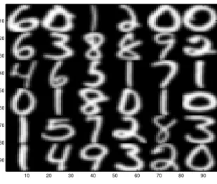
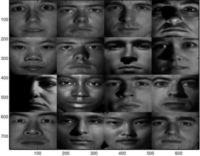
6.1.2 Datasets . . . 94
6.1.3 Clustering Computation and Evaluation . . . 96
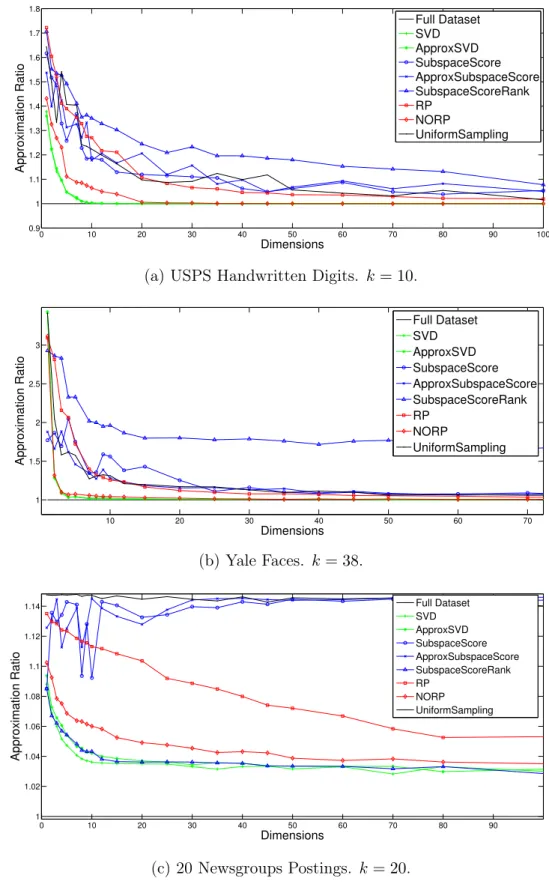
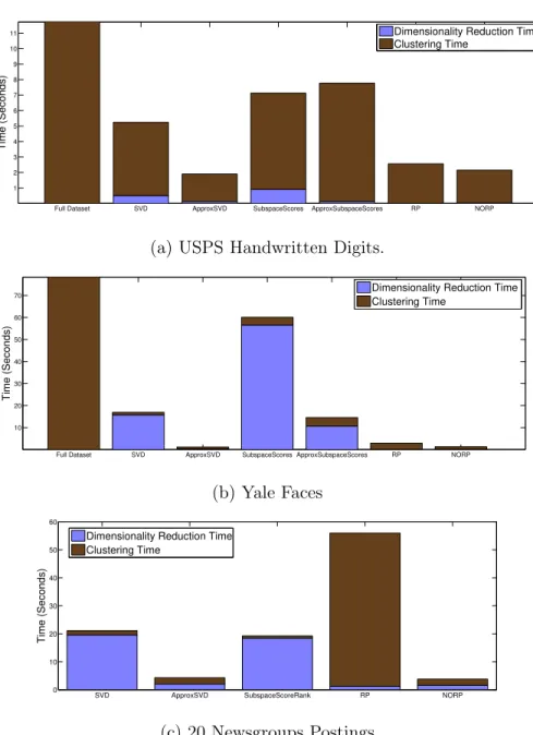
6.2 Comparision of Dimensionality Reduction Algorithms . . . 98
6.2.1 Dimension Versus Accuracy . . . 98
6.3 Tighter Understanding of SVD Based Dimensionality Reduction . . . 104
6.3.1 Comparision of Theoretical Bounds and Empirical Performance 105 6.4 Dimensionality Reduction Based Heuristics . . . 109
6.4.1 Lloyd’s Algorithm Initialization with Random Projection . . . 109
6.4.2 Related Heuristic Algorithms . . . 111
6.5 Empirical Conclusions . . . 111
7 Neurally Plausible Dimensionality Reduction and Clustering 113 7.1 Neural Principal Component Analysis. . . 113
7.2 Neural 𝑘-Means Clustering . . . 114
7.3 Neural Network Implementation of Lloyd’s Heuristic. . . 116
7.4 Overview of Proposed Neural Work . . . 117
8 Conclusion 119 8.1 Open Problems . . . 120
Chapter 1
Introduction
This thesis will focus on dimensionality reduction techniques for approximate 𝑘-means clustering. In this chapter, we introduce the 𝑘-means clustering problem, overview known algorithmic results, and discuss how algorithms can be accelerated using di-mensionality reduction. We then outline our contributions, which provide new the-oretical analysis along with empirical validation for a number of dimensionality re-duction algorithms. Finally we overview planned future work on neurally plausible algorithms for clustering and dimensionality reduction.
1.1
𝑘-Means Clustering
Cluster analysis is one of the most important tools in data mining and unsupervised machine learning. The goal is to partition a set of objects into subsets (clusters) such that the objects within each cluster are more similar to each other than to the objects in other clusters. Such a clustering can help distinguish various ‘classes’ within a dataset, identify sets of similar features that may be grouped together, or simply partition a set of objects based on some similarity criterion.
There are countless clustering algorithms and formalizations of the problem [JMF99]. One of the most common is 𝑘-means clustering [WKQ+08]. Formally, the goal is to partition 𝑛 vectors in R𝑑, {a
1, . . . , a𝑛}, into 𝑘 sets, {𝐶1, . . . , 𝐶𝑘}. Let 𝜇𝑖 be the cen-troid (the mean) of the vectors in 𝐶𝑖. Let A ∈ R𝑛×𝑑 be a data matrix containing our
vectors as rows and let 𝒞 represent the chosen partition into {𝐶1, . . . , 𝐶𝑘}. Then we seek to minimize the objective function:
𝐶𝑜𝑠𝑡(𝒞, A) = 𝑘 ∑︁ 𝑖=1 ∑︁ a𝑗∈𝐶𝑖 ‖a𝑗− 𝜇𝑖‖ 2 2 (1.1)
That is, the goal is to minimize the total intracluster variance of the data. This is equal to the sum of squared distances between the data points and the centroids of their assigned clusters. We will always use the squared Euclidean distance as our cost measure; however, this may be generalized. For example the problem may be defined using the Kullback-Leibler divergence, the squared Mahalanobis distance, or any Bregman divergance [BMDG05]. Our restriction of the problem, which is the most commonly studied, is sometimes referred to as Euclidean k-means clustering.
The 𝑘-means objective function is simple and very effective in a range of applica-tions, and so is widely used in practice and studied in the machine learning commu-nity [Jai10, Ste06, KMN+02a]. Applications include document clustering [SKK+00,
ZHD+01], image segmentation [RT99,NOF+06], color quantization in image
process-ing [KYO00, Cel09], vocabulary generation for speech recognition [WR85] and bag-of-words image classification [CDF+04]. Recently, it has also become an important
primitive in the theoretical computer science literature. Minimum cost, or approxi-mately minimum cost clusterings with respect to the 𝑘-means objective function can be shown to give provably good partitions of graphs into low expansion partitions - where each set of vertices has few outgoing edges compared with internal edges [PSZ14, CAKS15]. Under some conditions, 𝑘-means clustering a dataset generated by a mixture of Gaussian distributions can be used to estimate the parameters of the distribution to within provable accuracy [KK10].
Minimizing the 𝑘-means objective function is a geometric problem that can be solved exactly using Voronoi diagrams [IKI94]. Unfortunately, this exact algorithm requires time 𝑂(︀𝑛𝑂(𝑘𝑑))︀. In fact, 𝑘-means clustering is known to be NP-hard, even if we fix 𝑘 = 2 or 𝑑 = 2 [ADHP09, MNV09]. Even finding a cluster assignment achieving cost within (1 + 𝜖) of the optimal is NP-hard for some fixed 𝜖, ruling out
the possibility of a polynomial-time approximation scheme (PTAS) for the problem [ACKS15]. Given its wide applicability, overcoming these computational obstacles is an important area of research.
1.2
Previous Algorithmic Work
Practitioners almost universally tackle the 𝑘-means problem with Lloyd’s heuristic, which iteratively approximates good cluster centers [Llo82]. This algorithm is so popular that is it often referred to simply as the “𝑘-means algorithm” in the machine learning and vision communities [SKK+00, KYO00, CDF+04]. It runs in worst case exponential time, but has good smoothed complexity (i.e. polynomial runtime on small random perturbations of worst case inputs) and converges quickly in practice [Vas06]. However, the heuristic is likely to get stuck in local minima. Thus, finding provably accurate approximation algorithms is still an active area of research.
Initializing Lloyd’s algorithm using the widely implemented [Ope15,Sci15,Mat15a] k-means++ technique guarantees a log(𝑘) factor multiplicative approximation to the optimal cluster cost in expectation [Vas06]. Several (1 + 𝜖)-approximation algorithms are known, however they typically have exponential dependence on both 𝑘 and 𝜖 and are too slow to be useful in practice [KSS04, HPK07]. The best polynomial time approximation algorithm achieves a (9 + 𝜖)-approximation [KMN+02b]. Achieving a
(1 + 𝜖)-approximation is known to be NP-hard for some small constant 𝜖 [ACKS15], however closing the gap between this hardness result and the known (9+𝜖) polynomial time approximation algorithm is a very interesting open problem.
1.3
Dimensionality Reduction
In this thesis, we do not focus on specific algorithms for minimizing the 𝑘-means ob-jective function. Instead, we study techniques that can be used in a “black box" man-ner to accelerate any heuristic, approximate, or exact clustering algorithm. Specif-ically, we consider dimensionality reduction algorithms. Given a set of data points
{a1, . . . , a𝑛} in R𝑑, we seek to find a low-dimensional representation of these points that approximately preserves the 𝑘-means objective function. We show that, using common techniques such as random projection, principal component analysis, and feature sampling, one can quickly map these points to a lower dimensional point set, {˜a1, . . . , ˜a𝑛} in R𝑑
′
, with 𝑑′ << 𝑑. Solving the clustering problem on the low dimen-sional dataset will give an approximate solution for the original dataset. c In other words, we show how to obtain a sketch ˜A with many fewer columns than the original data matrix A. An optimal (or approximately optimal) 𝑘-means clustering for ˜A will also be approximately optimal for A. Along with runtime gains, working with the smaller dimension-reduced dataset ˜A can generically improve memory usage and data communication costs.
Using dimensionality reduction as a preprocessing step for clustering has been popular in practice for some time. The most common technique is to set ˜A to be A projected onto its top 𝑘 principal components [DH04]. Random projection based approaches have also been experimented with [FB03]. As far as we can tell, the first work that gives provable approximation bounds for a given sketching technique was [DFK+99], which demonstrates that projecting A to its top 𝑘 principal components
gives ˜A such that finding an optimal clustering over ˜A yields a clustering within a factor of 2 of the optimal for A. A number of subsequent papers have expanded on an improved this initial result, given provable bounds for techniques such as random projection and feature selection [BMD09, BZD10,BZMD11,FSS13]. Dimensionality reduction has also received considerable attention beyond the 𝑘-means clustering problem, in the study of fast linear algebra algorithms for problems such as matrix multiplication, regression, and low-rank approximation [HMT11, Mah11]. We will draw heavily on this work, helping to unify the study of 𝑘-means clustering and linear algebraic computation.
The types of dimensionality reduction studied in theory and practice generally fall into two categories. The columns of the sketch ˜A may be a small subset of the columns of A. This form of dimensionality reduction is known as feature selection - since the columns of A correspond to features of our original data points. To
form ˜A we have selected a subset of these features that contains enough information to compute an approximately optimal clustering on the full dataset. Alternatively, feature extraction refers to dimensionality reduction techniques where the columns of
˜
A are not simply a subset of the columns of A. They are a new set of features that have been extracted from the original dataset. Typically (most notably in the cases of random projection and principal component analysis), these extracted features are simply linear combinations of the original features.
1.4
Our Contributions
This thesis will first present a number of new theoretical results on dimensionality reduction for approximate 𝑘-means clustering. We show that common techniques such as random projection, principal component analysis, and feature sampling give provably good sketches, which can be used to find near optimal clusterings. We com-plement our theoretical results with an empirical evaluation of the dimensionality reduction techniques studied. Finally, we will discuss extensions to neural implemen-tations of 𝑘-means clustering algorithms and how these implemenimplemen-tations may be used in combination with neural dimensionality reduction.
1.4.1
Main Theoretical Results
The main theoretical results presented in this thesis are drawn from [CEM+15]. We show that 𝑘-means clustering can be formulated as a special case of a general con-strained low-rank approximation problem. We then define the concept of a projection-cost-preserving sketch - a sketch of A that can be used to approximately solve the constrained low-rank approximation problem. Finally, we show that a number of effi-cient techniques can be used to obtain projection-cost-preserving sketches. Since our sketches can be used to approximately solve the more general constrained low-rank approximation problem, they also apply to 𝑘-means clustering. We improve a number of previous results on dimensionality reduction for 𝑘-means clustering, as well as give
applications to streaming and distributed computation.
Constrained Low-Rank Approximation
A key observation, used in much of the previous work on dimensionality reduction for 𝑘-means clustering, is that 𝑘-means clustering is actually a special case of a more gen-eral constrained low-rank approximation problem [DFK+04]. A more formal definition will follow in the thesis body, however, roughly speaking, for input matrix A ∈ R𝑛×𝑑, this problem requires finding some 𝑘 dimensional subspace Z of R𝑛 minimizing the cost function:
‖A − PZA‖2𝐹.
PZA is the projection of A to the subspace Z and ‖ · ‖2𝐹 is the squared Frobenius norm - the sum of squared entries of a matrix. This cost function can also be referred to as the ‘distance’ from A to the subspace Z. Since Z is 𝑘 dimensional, PZA has rank 𝑘, so finding an optimal Z can be viewed as finding an optimal low-rank approximation of A, minimizing the Frobenius norm cost function.
As we will discuss in more detail in the thesis body, if Z is allowed to be any rank 𝑘 subspace of R𝑛, then this problem is equivalent to finding the best rank 𝑘 approximation of A. It is well known that the optimal Z is the subspace spanned by the top 𝑘 left principal components (also known as singular vectors) of A. Finding this subspace is achieved using principal component analysis (PCA), also known as singular value decomposition (SVD). Hence finding an approximately optimal Z is often referred to as approximate PCA or approximate SVD.
More generally, we may require that Z is chosen from any subset of subspaces in R𝑛. This additional constraint on Z gives us the constrained low-rank approximation problem. We will show that 𝑘-means clustering is a special case of the constrained low-rank approximation problem, where the choice of Z is restricted to a specific set of subspaces. Finding the optimal Z in this set is equivalent to finding the clustering 𝒞 minimizing the 𝑘-means cost function (1.1) for A. Other special cases of constrained
low-rank approximation include problems related to sparse and nonnegative PCA [PDK13, YZ13,APD14].
Projection-Cost-Preserving Sketches
After formally defining constrained low-rank approximation and demonstrating that 𝑘-means clustering is a special case of the problem, we will introduce the concept of a projection-cost-preserving sketch. This is a low dimensional sketch ˜A ∈ R𝑛×𝑑′ of our original dataset A ∈ R𝑛×𝑑 such that the distance of ˜A from any 𝑘-dimensional subspace is within a (1 ± 𝜖) multiplicative factor of that of A. Intuitively, this means that ˜A preserves the objective function of the constrained low-rank approximation problem. So, we can approximately solve this problem using ˜A in place of A. As 𝑘-means clustering is a special case of constrained low-rank approximation, ˜A gives a set of low dimensional data points that can be used to find an approximately optimal 𝑘-means clustering on our original data points.
We give several simple and efficient approaches for computing a projection-cost-preserving sketch of a matrix A. As is summarized in Table 1.1, and detailed in Chapter 4, our results improve most of the previous work on dimensionality reduc-tion for 𝑘-means clustering. We show generally that a sketch ˜A with only 𝑑′ = 𝑂(𝑘/𝜖2) columns suffices for approximating constrained low-rank approximation, and hence 𝑘-means clustering, to within a multiplicative factor of (1 + 𝜖). Most of our techniques simply require computing an SVD of A, multiplying A by a random projection ma-trix, randomly sampling columns of A, or some combination of the three. These methods have well developed implementations, are robust, and can be accelerated for sparse or otherwise structured data. As such, we do not focus heavily on specific implementations or runtime analysis. We do show that our proofs are amenable to approximation and acceleration in the underlying sketching techniques – for exam-ple, it is possible to use fast approximate SVD algorithms, sparse random projection matrices, and inexact sampling probabilities.
Previous Work Our Results
Technique Ref. Dimension Error Theorem Dimension Error
SVD [DFK +04] [FSS13] 𝑘 𝑂(𝑘/𝜖2) 2 1 + 𝜖 Thm 17 ⌈𝑘/𝜖⌉ 1 + 𝜖 Approximate SVD [BZMD11] 𝑘 2 + 𝜖 Thm 18,19 ⌈𝑘/𝜖⌉ 1 + 𝜖 Random Projection [BZD10] 𝑂(𝑘/𝜖 2) 2 + 𝜖 Thm 22 Thm 32 𝑂(𝑘/𝜖2) 𝑂(log 𝑘/𝜖2) 1 + 𝜖 9 + 𝜖† Non-oblivious Randomized Projection [Sar06] 𝑂(𝑘/𝜖) 1 + 𝜖‡ Thm 26 𝑂(𝑘/𝜖) 1 + 𝜖 Feature Selection (Random Sampling) [BMD09, BZMD11] 𝑂 (︀𝑘 log 𝑘 𝜖2 )︀ 3 + 𝜖 Thm 24 𝑂(︀𝑘 log 𝑘 𝜖2 )︀ 1 + 𝜖 Feature Selection (Deterministic) [BMI13] 𝑘 < 𝑟 < 𝑛 𝑂(𝑛/𝑟) Thm 25 𝑂(𝑘/𝜖 2) 1 + 𝜖
Table 1.1: Summary of our new dimensionality reduction results. Dimension refers to the number of columns 𝑑′ required for a projection-cost-preserving sketch ˜A computed using the corresponding technique. As noted, two of the results do not truely give projection-cost-preserving sketches, but are relevant for the special cases of 𝑘-means clustering and uncontrained low-rank approximation (i.e. approximate SVD) only.
Application of Results
In addition to providing improved results on dimensionality reduction for approx-imating the constrained low-rank approximation problem, our results have several applications to distributed and streaming computation, which we cover in Chapter5. One example of our new results is that a projection-cost-preserving sketch which allows us to approximate constrained low-rank approximation to within a multiplica-tive factor of (1 + 𝜖) can be obtained by randomly projecting A’s rows to 𝑂(𝑘/𝜖2) dimensions – i.e. multiplying on the right by a random Johnson-Lindenstrauss matrix with 𝑂(𝑘/𝜖2) columns. This random matrix can be generated independently from A and represented with very few bits. If the rows of A are distributed across multi-ple servers, multiplication by this matrix may be done independently by each server.
Running a distributed clustering algorithm on the dimension-reduced data yields the lowest communication relative error distributed algorithm for 𝑘-means, improving on [LBK13, BKLW14, KVW14].
As mentioned, constrained low-rank approximation also includes unconstrained low-rank approximation (i.e. principal component analysis) as a special case. Since the Johnson-Lindenstrauss matrix in the above result is chosen without looking at A, it gives the first oblivious dimension reduction technique for principal component analysis. This technique yields an alternative to the algorithms in [Sar06, CW13,
NN13] that has applications in the streaming setting, which will also be detailed in the thesis body.
Finally, in addition to the applications to 𝑘-means clustering and low-rank ap-proximation, we hope that projection-cost-preserving sketches will be useful in de-veloping future randomized matrix algorithms. These sketches relax the guaran-tee of subspace embeddings, which have received significant attention in recent years [Sar06, CW13, LMP13, MM13, NN13]. Subspace embedding sketches require that ‖x ˜A‖2 ≈ ‖xA‖2 simultaneously for all x. It is not hard to show that this is equiv-alent to ˜A preserving the distance of A to any subspace in R𝑛. In general ˜A will require at least 𝑂(𝑟𝑎𝑛𝑘(A)) columns. On the other hand, projection-cost-preserving sketches only preserve the distance to subspaces with dimension at most 𝑘, however they also require only 𝑂(𝑘) columns.
1.4.2
Empirical Evaluation
After presenting the theoretical results obtained in [CEM+15], we provide an
empir-ical evaluation of these results. The dimensionality reduction algorithms studied are generally simple and rely on widely implemented primitives such as the singular value decomposition and random projection. We believe they are likely to be useful in prac-tice. Empirical work on some of these algorithms exists [BZMD11, CW12, KSS15],
however we believe that further work in light of the new theoretical results is valuable. We first implement most of the dimensionality reduction algorithms that we give the-oretical bounds for. We compare dimensionality reduction runtimes and accuracy when applied to 𝑘-means clustering, confirming the strong empirical performance of the majority of these algorithms. We find that two approaches – Approximate SVD and Non-Oblivous Random Projection (which had not been previously considered for 𝑘-means clustering) are particularly appealing in practice as they combine ex-tremely fast dimensionality reduction runtime with very good accuracy when applied to clustering.
Dimensionality Reduction via the Singular Value Decomposition
After implementing and testing a number of dimensionality reduction algorithms, we take a closer look at one of the most effective techniques – dimensionality reduction using the SVD. In [CEM+15] we show that the best ⌈𝑘/𝜖⌉-rank approximation to A (identified using the SVD) gives a projection-cost-preserving sketch with (1 + 𝜖) multiplicative error. This is equivalent to projecting A onto its top ⌈𝑘/𝜖⌉ singular vectors (or principal components.)
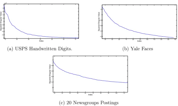
Our bound improves on [FSS13], which requires an 𝑂(𝑘/𝜖2) rank approximation. 𝑘 is typically small so the lack of constant factors and 1/𝜖 dependence (vs. 1/𝜖2) can be significant in practice. Our analysis also shows that a smaller sketch suffices when A’s spectrum is not uniform, a condition that is simple to check in practice. Specifically, if the singular values of A decay quickly, or A has a heavy singular value ‘tail’, two properties that are very common in real datasets, a sketch of size 𝑜(𝑘/𝜖) may be used.
We demonstrate that, for all datasets considered, due to spectral decay and heavy singular value tails, a sketch with only around 2𝑘 to 3𝑘 dimensions provably suffices for very accurate approximation of an optimal 𝑘-means clustering. Empirically, we
confirm that even smaller sketches give near optimal clusterings.
Interestingly, SVD based dimensionality reduction is already popular in practice as a preprocessing step for 𝑘-means clustering. It is viewed as both a denoising technique and a way of approximating the optimal clustering while working with a lower dimensional dataset [DH04]. However, practitioners typically project to exactly 𝑘 dimensions (principal components), which is a somewhat arbitrary choice. Our new results clarify the connection between PCA and 𝑘-means clustering and show exactly how to choose the number of principal components to project down to in order to find an approximately optimal clustering.
Dimensionality Reduction Based Heuristics
In practice, dimensionality reduction may be used in a variety of ways to accelerate 𝑘-means clustering algorithms. The most straightforward technique is to produce a projection-cost-preserving sketch with one’s desired accuracy, run a 𝑘-means cluster-ing algorithm on the sketch, and output the nearly optimal clusters obtained. However a number of heuristic dimension-reduction based algorithms may also be useful. In the final part of our empirical work, we implement and evaluate one such algorithm. Specifically, we reduce our data points to an extremely low dimension, compute an approximate clustering in the low dimensional space, and then use the computed cluster centers to initialize Lloyd’s heuristic on the full dataset. We find that this technique can outperform the popular k-means++ initialization step for Lloyd’s al-gorithm, with a similar runtime cost. We also discuss a number of related algorithms that may be useful in practice for clustering very large datasets.
1.4.3
Neural Clustering Algorithms
After presenting a theoretical and empirical evaluation of dimensionality reduction for 𝑘-means clustering, we will discuss possible extensions of our work to a neural setting.
In future work, we plan to focus on developing a neurally plausible implementation of a 𝑘-means clustering algorithm with dimensionality reduction. We hope to show that this implementation can be used for concept learning in the brain.
Dimensionality Reduction and Random Projection in the Brain
It is widely accepted that dimensionality reduction is used throughout the human brain and is a critical step in information processing [GS12a, SO01]. For exam-ple, image acquisition in the human brain involves input from over 100 million pho-toreceptor cells [Hec87]. Efficiently processing the input from these receptors, and understanding the image in terms of high level concepts requires some form of di-mensionality reduction. To evidence this fact, only 1/100𝑡ℎ as many optic nerve cells exist to transmit photoreceptor input as photoreceptors themselves, possibly indi-cating a significant early stage dimensionality reduction in visual data [AZGMS14]. Similar dimensionality reduction may be involved in auditory and tactile perception, as well is in ‘internal’ data processing such as in the transmission of control informa-tion from the large number of neurons in the motor cortex to the smaller spinal cord [AZGMS14].
One hypothesis is that dimensionality reduction using random projection is em-ployed widely in the brain [GS12a, AV99]. Randomly projecting high dimensional input data to a lower dimensional space can preserve enough information to approx-imately recover the original input if it is sparse in some basis [GS12a], or to learn robust concepts used to classify future inputs [AV99]. Further, random projection can be naturally implemented by randomly connecting a large set of input neurons with a small set of output neurons, which represent the dimension-reduced input [AV99]. Some recent work has focused on showing that more efficient implementations, with a limited number of random connections, are in fact possible in realistic neural networks [AZGMS14].
Combining Neurally Plausible Dimensionality Reduction with Clustering
Recall that one of our main results shows that applying a random projection with 𝑂(𝑘/𝜖2) dimensions to our dataset gives a projection-cost-preserving sketch that al-lows us to solve 𝑘-means to within a (1 + 𝜖) multiplicative factor. A natural question is how random projection in the brain may be combined with neural algorithms for clustering. Can we develop neurally plausible 𝑘-means clustering algorithms that use random projection as a dimensionality reducing preprocessing step? Might a dimen-sionality reduction-clustering pipeline be used for concept learning in the brain? For example, we can imagine that over time a brain is exposed to successive inputs from a large number of photoreceptor cells which undergo significant initial dimensionality reduction using random projection. Can we cluster these successive (dimensional-ity reduced) inputs to learning distinct concept classes corresponding to everyday objects? We discuss potential future work in this area in Chapter 7.
Chapter 2
Mathematical Preliminaries
In this chapter we review linear algebraic notation and preliminaries that we will refer back to throughout this thesis.
2.1
Basic Notation and Linear Algebra
For a vector x ∈ R𝑛×1 we use x
𝑖 to denote the 𝑖𝑡ℎ entry of the vector. For a matrix M ∈ R𝑛×𝑑 we use M
𝑖𝑗 to denote the entry in M’s 𝑖𝑡ℎ row and 𝑗𝑡ℎ column. We use m𝑖 to denote M’s 𝑖𝑡ℎrow. M⊤
∈ R𝑑×𝑛is the transpose of M with M⊤
𝑖𝑗 = M𝑗𝑖. Intuitively it is the matrix reflected over its main diagonal. For a vector x, the squared Euclidean norm is given by ‖x‖22 = x⊤x = ∑︀𝑛𝑖=1x2𝑖.
For square M ∈ R𝑛×𝑛, the trace of M is defined as tr(M) = ∑︀𝑛
𝑖=1M𝑖𝑖 – the sum of M’s diagonal entries. Clearly, the trace is linear so for any M, N ∈ R𝑛×𝑛, tr(M + N) = tr(M) + tr(N). The trace also has the following very useful cyclic property:
Lemma 1 (Cyclic Property of the Trace). For any M ∈ R𝑛×𝑑 and N ∈ R𝑑×𝑛, tr(MN) = tr(NM).
the trace is invariant under cyclic permutations. E.g. for any M, N, K, tr(MNK) = tr(KMN) = tr(NKM). Proof. tr(MN) = 𝑛 ∑︁ 𝑖=1 (MN)𝑖𝑖 = 𝑛 ∑︁ 𝑖=1 𝑑 ∑︁ 𝑗=1
M𝑖𝑗N𝑗𝑖 (Definition of matrix multiplication)
= 𝑑 ∑︁ 𝑗=1 𝑛 ∑︁ 𝑖=1
M𝑖𝑗N𝑗𝑖 (Switching order of summation)
= 𝑑 ∑︁ 𝑗=1
(NM)𝑗𝑗 = tr(NM). (Definition of matrix multiplication and trace)
If M ∈ R𝑛×𝑛 is symmetric, then all of its eigenvalues are real. It can be writ-ten using the eigendecompostion M = VΛV⊤ where V has orthonormal columns (the eigenvectors of M) and Λ is a diagonal matrix containing the eigenvalues of M [TBI97]. We use 𝜆𝑖(M) to denote the 𝑖th largest eigenvalue of M in absolute value.
2.2
The Singular Value Decomposition
The most important linear algebraic tool we will use throughout our analysis is the singular value decomposition (SVD). For any 𝑛 and 𝑑, consider a matrix A ∈ R𝑛×𝑑. Let 𝑟 = rank(A). By the singular value decomposition theorem [TBI97], we can write A = UΣV⊤. The matrices U ∈ R𝑛×𝑟 and V ∈ R𝑑×𝑟 each have orthonormal columns – the left and right singular vectors of A respectively. The columns of U form an orthonormal basis for the column span of A, while the columns of V form an orthonormal basis for the A’s row span. Σ ∈ R𝑟×𝑟 is a positive diagonal matrix with Σ𝑖𝑖 = 𝜎𝑖, where 𝜎1 ≥ 𝜎2 ≥ ... ≥ 𝜎𝑟 are the singular values of A. If A is symmetric,
the columns of U = V are just the eigenvectors of A and the singular values are just the eigenvalues.
We will sometimes use the pseudoinverse of A, which is defined using the SVD.
Definition 2 (Matrix Pseudoinverse). For any A ∈ R𝑛×𝑑 with singular value decom-position A = UΣV⊤, the pseudoinverse of A is given by A+= VΣ−1U⊤, where Σ−1 is the diagonal matrix with Σ−1𝑖𝑖 = 1/𝜎𝑖.
If A is invertible, then A+ = A−1. Otherwise, A+ acts as an inverse for vectors in the row span of A. Let I denote the identity matrix of appropriate size in the following equations. For any x in the row span of A,
A+Ax = VΣ−1U⊤UΣV⊤x (Definition of psuedoinverse and SVD of A)
= VΣ−1IΣV⊤xx (U⊤U = I since it has orthonormal columns)
= VV⊤x (Σ−1IΣ = I since Σ𝑖𝑖· Σ−1𝑖𝑖 = 1)
= x.
The last equality follows because x is in the rowspan of A. Since the columns of V form an orthonormal basis for this span, we can write x = Vy for some y and have: VV⊤x = VV⊤Vy = VIy = x.
While we will not specifically use this fact in our analysis, it is worth understanding why singular value decomposition is often referred to as principal component analysis (PCA). The columns of U and V are known as the left and right principal components of A. v1, the first column of V, is A’s top right singular vector and provides a top principal component, which describes the direction of greatest variance within A. The 𝑖th singular vector v𝑖 provides the 𝑖th principal component, which is the direction
of greatest variance orthogonal to all higher principal components. Formally: ‖Av𝑖‖22 = v ⊤ 𝑖 A ⊤ Av𝑖 = 𝜎𝑖2 = max x:‖x‖2=1 x⊥v𝑗 ∀𝑗<𝑖 x⊤A⊤Ax, (2.1)
where A⊤A is the covariance matrix of A. Similarly, for the left singular vectors we have:
‖u⊤𝑖 A‖22 = u⊤𝑖 AA⊤u𝑖 = 𝜎𝑖2 = max
x:‖x‖2=1 x⊥u𝑗 ∀𝑗<𝑖
x⊤AA⊤x. (2.2)
2.3
Matrix Norms and Low-Rank Approximation
A’s squared Frobenius norm is given by summing its squared entries: ‖A‖2 𝐹 = ∑︀ 𝑖,𝑗A 2 𝑖,𝑗 = ∑︀
𝑖‖a𝑖‖22, where a𝑖 is the 𝑖𝑡ℎ row of A. We also have the identities: ‖A‖2
𝐹 = tr(AA⊤) = ∑︀
𝑖𝜎 2
𝑖. So the squared Frobenius norm is the sum of squared singular values. A’s spectral norm is given by ‖A‖2 = 𝜎1, its largest singular value. Equivalently, by the ‘principal component’ characterization of the singular values in (2.2), ‖A‖2 = maxx:‖x‖2=1‖Ax‖2. Let Σ𝑘 ∈ R
𝑘×𝑘 be the upper left submatrix of Σ containing just the largest 𝑘 singular values of A. Let U𝑘 ∈ R𝑛×𝑘 and V𝑘 ∈ R𝑑×𝑘 be the first 𝑘 columns of U and V respectively. For any 𝑘 ≤ 𝑟, A𝑘 = U𝑘Σ𝑘V𝑘⊤ is the closest rank 𝑘 approximation to A for any unitarily invariant norm, including the Frobenius norm and spectral norm [Mir60]. That is,
‖A − A𝑘‖𝐹 = min
B|rank(B)=𝑘‖A − B‖𝐹 and ‖A − A𝑘‖2 = min
B|rank(B)=𝑘‖A − B‖2.
We often work with the remainder matrix A − A𝑘 and label it A𝑟∖𝑘. We also let U𝑟∖𝑘 and V𝑟∖𝑘 denote the remaining 𝑟 − 𝑘 columns of U and V and Σ𝑟∖𝑘 denote the
lower 𝑟 − 𝑘 entries of Σ.
We now give two Lemmas that we use repeatedly to work with matrix norms.
Lemma 3 (Spectral Submultiplicativity). For any two matrices M ∈ R𝑛×𝑑 and N ∈ R𝑑×𝑝, ‖MN‖𝐹 ≤ ‖M‖𝐹‖N‖2 and ‖MN‖𝐹 ≤ ‖N‖𝐹‖M‖2.
This property is known as spectral submultiplicativity. It holds because multiplying by a matrix can scale each row or column, and hence the Frobenius norm, by at most the matrix’s spectral norm.
Proof. ‖MN‖2 𝐹 = ∑︁ 𝑖 ‖ (MN)𝑖‖2
2 (Frobenius norm is sum of row norms)
=∑︁ 𝑖 ‖m𝑖N‖22 (𝑖𝑡ℎ row of MN equal to m𝑖N) ≤∑︁ 𝑖 ‖m𝑖‖22· 𝜎 2 1(N) = 𝜎 2 1(N) · ∑︁ 𝑖 ‖m𝑖‖22 = ‖M‖ 2 𝐹‖N‖ 2 2.
Taking square roots gives the final bound. The inequality follows from (2.2) which says that ‖xN‖2
2 ≤ 𝜎12(N) for any unit vector x. By rescaling, for any vector x, ‖xN‖22 ≤ ‖x‖2
2· 𝜎12(N) = ‖x‖22‖N‖22.
Lemma 4 (Matrix Pythagorean Theorem). For any two matrices M and N with the same dimensions and MN⊤ = 0 then ‖M + N‖2
𝐹 = ‖M‖2𝐹 + ‖N‖2𝐹.
Proof. This matrix Pythagorean theorem follows from the fact that ‖M + N‖2 𝐹 = tr((M + N)(M + N)⊤) = tr(MM⊤+ NM⊤+ MN⊤+ NN⊤) = tr(MM⊤) + tr(0) + tr(0) + tr(NN⊤) = ‖M‖2𝐹 + ‖N‖2𝐹.
Finally, we define the Loewner ordering, which allows us to compare two matrices in ‘spectral sense’:
Definition 5 (Loewner Ordering on Matrices). For any two symmetric matrices M, N ∈ R𝑛×𝑛, M ⪯ N indicates that N − M is positive semidefinite. That is, it has all nonnegative eigenvalues and x⊤(N − M)x ≥ 0 for all x ∈ R𝑛.
Note that we can view the spectral norm of a matrix as spectrally bounding that matrix with respect to the identity. Specifically, if ‖M‖2 ≤ 𝜆, then for any x, x⊤Mx ≤ 𝜆 so −𝜆 · I ⪯ M ⪯ 𝜆 · I. We will also use the following simple Lemma about the Loewner ordering:
Lemma 6. For any M, N ∈ R𝑛×𝑛, if M ⪯ N then for any D ∈ R𝑛×𝑑:
D⊤MD ⪯ D⊤ND.
Proof. This is simply because, letting y = Dx,
x⊤(︀D⊤ND − D⊤MD)︀ x = y⊤(N − M) y ≥ 0
where the last inequality follow from the definition of M ⪯ N.
2.4
Orthogonal Projection
We often use P ∈ R𝑛×𝑛 to denote an orthogonal projection matrix, which is any ma-trix that can be written as P = QQ⊤ where Q ∈ R𝑛×𝑘 is a matrix with orthonormal columns. Multiplying a matrix by P on the left will project its columns to the column span of Q. Since Q has 𝑘 columns, the projection has rank 𝑘. The matrix I − P is also an orthogonal projection of rank 𝑛 − 𝑘 onto the orthogonal complement of the column span of Q.
Orthogonal projection matrices have a number of important properties that we will use repeatedly.
Lemma 7 (Idempotence of Projection). For any orthogonal projection matrix P ∈ R𝑛×𝑛, we have
P2 = P.
Intuitively, if we apply a projection twice, this will do nothing more than if we have just applied it once.
Proof.
P2 = QQ⊤QQ⊤ = QIQ⊤ = P.
Lemma 8 (Projection Decreases Frobenius Norm). For any A ∈ R𝑛×𝑑 and any orthogonal projection matrix P ∈ R𝑛×𝑛,
‖PA‖2𝐹 ≤ ‖A‖2𝐹.
Proof. We can write an SVD of P as P = QIQ⊤. So, P has all singular values equal to 1 and by spectral submultiplicativity (Lemma3), multiplying by P can only decrease Frobenius norm.
Lemma 9 (Separation into Orthogonal Components). For any orthogonal projection matrix P ∈ R𝑛×𝑛 we have (I − P)P = 0 and as a consequence, for any A ∈ R𝑛×𝑑 can write:
‖A‖2
𝐹 = ‖PA‖2𝐹 + ‖(I − P)A‖2𝐹.
Proof. The first claim follows because (I − P)P = P − P2 = P − P = 0. Intuitively, the columns of P fall within the column span of Q. The columns of I − P fall in the orthogonal complement of this span, and so are orthogonal to the columns of P.
(PA)⊤(I − P)A = A⊤P(I − P)A = 0 so: ‖A‖2 𝐹 = ‖PA + (I − P)A‖ 2 𝐹 = ‖PA‖ 2 𝐹 + ‖(I − P)A‖ 2 𝐹.
As an example application of Lemma 9, note that A𝑘 is an orthogonal projection of A: A𝑘 = U𝑘U⊤𝑘A. A𝑟∖𝑘 is its residual, A − A𝑘 = (I − U𝑘U⊤𝑘)A. Thus, ‖A𝑘‖2𝐹 + ‖A𝑟∖𝑘‖2𝐹 = ‖A𝑘+ A𝑟∖𝑘‖2𝐹 = ‖A‖2𝐹.
Chapter 3
Constrained Low-Rank
Approximation and
Projection-Cost-Preservation
In this chapter we will present the core of our theoretical results, developing the theory behind constrained low-rank approximation and its approximation using projection-cost-preserving sketches. The chapter is laid out as follows:
Section 3.1 We introduce constrained low-rank approximation and demonstrate that 𝑘-means clustering is a special case of the problem.
Section 3.2 We introduce projection-cost-preserving sketches and demonstrate how they can be applied to find nearly optimal solutions to constrained low-rank approximation.
Section 3.3 We give a high level overview of our approach to proving that common dimensionality reduction techniques yield projection-cost-preserving sketches. Formally, we give a set of sufficient conditions for a sketch ˜A to be projection-cost-preserving.
3.1
Constrained Low-Rank Approximation
We start by defining the constrained low-rank approximation problem and demon-strate that 𝑘-means clustering is a special case of this problem.
Definition 10 (Constrained 𝑘-Rank Approximation). For any A ∈ R𝑛×𝑑 and any set 𝑆 of rank 𝑘 orthogonal projection matrices in R𝑛×𝑛, the constrained 𝑘 rank ap-proximation problem is to find:
P* = arg min P∈𝑆
‖A − PA‖2
𝐹. (3.1)
That is, we want to find the projection in 𝑆 that best preserves A in the Frobenius norm. We often write Y = I𝑛×𝑛− P and refer to ‖A − PA‖2
𝐹 = ‖YA‖2𝐹 as the cost of the projection P.
When 𝑆 is the set of all rank 𝑘 orthogonal projections, this problem is equivalent to finding the optimal rank 𝑘 approximation for A, and is solved by computing U𝑘 using an SVD algorithm and setting P* = U𝑘U⊤𝑘. In this case, the cost of the optimal projection is ‖A − U𝑘U⊤𝑘A‖2𝐹 = ‖A𝑟∖𝑘‖2𝐹. As the optimum cost in the unconstrained case, ‖A𝑟∖𝑘‖2𝐹 is a universal lower bound on ‖A − PA‖2𝐹.
3.1.1
𝑘-Means Clustering as Constrained Low-Rank
Approxi-mation
The goal of 𝑘-means clustering is to partition 𝑛 vectors in R𝑑, {a
1, . . . , a𝑛}, into 𝑘 cluster sets, 𝒞 = {𝐶1, . . . , 𝐶𝑘}. Let 𝜇𝑖 be the centroid of the vectors in 𝐶𝑖. Let A ∈ R𝑛×𝑑 be a data matrix containing our vectors as rows and let 𝐶(a𝑗) be the set that vector a𝑗 is assigned to. The objective is to minimize the function given in (1.1):
𝐶𝑜𝑠𝑡(𝒞, A) = 𝑘 ∑︁ 𝑖=1 ∑︁ a𝑗∈𝐶𝑖 ‖a𝑗 − 𝜇𝑖‖ 2 2 = 𝑛 ∑︁ 𝑗=1 ‖a𝑗− 𝜇𝐶(a𝑗)‖ 2 2.
To see that 𝑘-means clustering is an instance of general constrained low-rank approximation, we rely on a linear algebraic formulation of the 𝑘-means objective that has been used critically in prior work on dimensionality reduction for the problem (see e.g. [BMD09]).
For a clustering 𝒞 = {𝐶1, . . . , 𝐶𝑘}, let X𝒞 ∈ R𝑛×𝑘 be the cluster indicator matrix, with X𝒞(𝑗, 𝑖) = 1/√︀|𝐶𝑖| if a𝑗 is assigned to 𝐶𝑖. X𝒞(𝑗, 𝑖) = 0 otherwise. Thus, X⊤𝒞A has its 𝑖𝑡ℎ row equal to √︀|𝐶𝑖| · 𝜇
𝑖 and X𝒞X ⊤
𝒞A has its 𝑗th row equal to 𝜇𝐶(a𝑗), the
center of a𝑗’s assigned cluster. So we can express the 𝑘-means objective function as:
‖A − X𝒞X⊤𝒞A‖2𝐹 = 𝑛 ∑︁
𝑗=1
‖a𝑗− 𝜇𝐶(a𝑗)‖22.
By construction, the columns of X𝒞 have disjoint supports and have norm 1, so are orthonormal vectors. Thus X𝒞X⊤𝒞 is an orthogonal projection matrix with rank 𝑘, and 𝑘-means is just the constrained low-rank approximation problem of (3.1) with 𝑆 as the set of all possible cluster projection matrices X𝒞X⊤𝒞.
While the goal of 𝑘-means is to well approximate each row of A with its clus-ter cenclus-ter, this formulation shows that the problem actually amounts to finding an optimal rank 𝑘 subspace to project the columns of A to. The choice of subspace is constrained because it must be spanned by the columns of a cluster indicator matrix.
3.2
Projection-Cost-Preserving Sketches
With the above reduction in hand, our primary goal now shifts to studying dimension-ality reduction for constrained low-rank approximation. All results will hold for the important special cases of 𝑘-means clustering and unconstrained low-rank approxima-tion. We aim to find an approximately optimal constrained low-rank approximation (3.1) for A by optimizing P (either exactly or approximately) over a sketch ˜A ∈ R𝑛×𝑑′
with 𝑑′ ≪ 𝑑. That is we want to solve:
˜
P* = arg min P∈𝑆
‖ ˜A − P ˜A‖2𝐹.
and be guaranteed that ‖A − ˜P*A‖2𝐹 ≤ (1 + 𝜖)‖A − P*A‖2
𝐹 for some approximation factor 𝜖 > 0.
This approach will certainly work if the cost ‖ ˜A − P ˜A‖2
𝐹 approximates the cost ‖A − PA‖2
𝐹 for every P ∈ 𝑆. If this is the case, choosing an optimal P for ˜A will be equivalent to choosing a nearly optimal P for A. An even stronger requirement is that ˜A approximates projection-cost for all rank 𝑘 projections P (of which 𝑆 is a subset). We call such an ˜A a projection-cost-preserving sketch.
Definition 11 (Rank 𝑘 Projection-Cost-Preserving Sketch with Two-sided Error). ˜
A ∈ R𝑛×𝑑′ is a rank 𝑘 projection-cost-preserving sketch of A ∈ R𝑛×𝑑 with error 0 ≤ 𝜖 < 1 if, for all rank 𝑘 orthogonal projection matrices P ∈ R𝑛×𝑛,
(1 − 𝜖)‖A − PA‖2𝐹 ≤ ‖ ˜A − P ˜A‖2𝐹 + 𝑐 ≤ (1 + 𝜖)‖A − PA‖2𝐹,
for some fixed non-negative constant 𝑐 that may depend on A and ˜A but is independent of P.
Note that ideas similar to projection-cost preservation have been considered in previous work. In particular, our definition is equivalent to the Definition 2 of [FSS13] with 𝑗 = 𝑘 and 𝑘 = 1. It can be strengthened slightly by requiring a one-sided error bound, which some of our sketching methods will achieve. The tighter bound is required for results that do not have constant factors in the sketch size (i.e. sketches with dimension exactly ⌈𝑘/𝜖⌉ rather than 𝑂(𝑘/𝜖)).
Definition 12 (Rank 𝑘 Projection-Cost-Preserving Sketch with One-sided Error). ˜
error 0 ≤ 𝜖 < 1 if, for all rank 𝑘 orthogonal projection matrices P ∈ R𝑛×𝑛, ‖A − PA‖2 𝐹 ≤ ‖ ˜A − P ˜A‖ 2 𝐹 + 𝑐 ≤ (1 + 𝜖)‖A − PA‖ 2 𝐹,
for some fixed non-negative constant 𝑐 that may depend on A and ˜A but is independent of P.
3.2.1
Application to Constrained Low-Rank Approximation
It is straightforward to show that a projection-cost-preserving sketch is sufficient for approximately optimizing (3.1), our constrained low-rank approximation problem.
Lemma 13 (Constrained Low-Rank Approximation via Projection-Cost-Preserving Sketches). For any A ∈ R𝑛×𝑑and any set 𝑆 of rank 𝑘 orthogonal projections, let P* = arg minP∈𝑆‖A − PA‖2
𝐹. Accordingly, for any ˜A ∈ R𝑛×𝑑
′
, let ˜P* = arg minP∈𝑆‖ ˜A − P ˜A‖2𝐹. If ˜A is a rank 𝑘 projection-cost preserving sketch for A with error 𝜖 (i.e. satisfies Definition 11), then for any 𝛾 ≥ 1, if ‖ ˜A − ˜P ˜A‖2𝐹 ≤ 𝛾‖ ˜A − ˜P*A‖˜ 2𝐹 ,
‖A − ˜PA‖2𝐹 ≤ (1 + 𝜖)
(1 − 𝜖) · 𝛾‖A − P *
A‖2𝐹.
That is, if ˜P is an optimal solution for ˜A, then it is also approximately optimal for A. We introduce the 𝛾 parameter to allow ˜P to be approximately optimal for ˜A. This ensures that our dimensionality reduction algorithms can be used as a preprocessing step for both exact and approximate constrained low-rank approximation (e.g. 𝑘-means clustering) algorithms. In the case of heuristics like Lloyd’s algorithm, while a provable bound on 𝛾 may be unavailable, the guarantee still ensures that if ˜P is a good low-rank approximation of ˜A, then it will also give a good low-rank approximation for A.
Proof. By optimality of ˜P* for ˜A, ‖ ˜A − ˜P*A‖˜ 2
𝐹 ≤ ‖ ˜A − P *A‖˜ 2
𝐹 and thus,
‖ ˜A − ˜P ˜A‖2𝐹 ≤ 𝛾‖ ˜A − P*A‖˜ 2𝐹. (3.2)
Further, since ˜A is projection-cost-preserving, the following two inequalities hold:
‖ ˜A − P*A‖˜ 2𝐹 ≤ (1 + 𝜖)‖A − P*A‖2𝐹 − 𝑐, (3.3)
‖ ˜A − ˜P ˜A‖2𝐹 ≥ (1 − 𝜖)‖A − ˜PA‖2𝐹 − 𝑐. (3.4)
Combining (3.2),(3.3), and (3.4), we see that:
(1 − 𝜖)‖A − ˜PA‖2𝐹 − 𝑐 ≤ ‖ ˜A − ˜P ˜A‖2𝐹 (By (3.4)) ≤ 𝛾‖ ˜A − P*A‖˜ 2𝐹 (By (3.2)) ≤ (1 + 𝜖) · 𝛾‖A − P*A‖2𝐹 − 𝛾𝑐 (By (3.3)) ‖A − ˜PA‖2𝐹 ≤ (1 + 𝜖)
(1 − 𝜖) · 𝛾‖A − P *
A‖2𝐹,
where the final step is simply the consequence of 𝑐 ≥ 0 and 𝛾 ≥ 1.
For any 0 ≤ 𝜖′ < 1, to achieve a (1 + 𝜖′)𝛾 approximation with Lemma 13, we just need 1+𝜖1−𝜖 = 1 + 𝜖′ and so must set 𝜖 = 2+𝜖𝜖′ ′ ≥
𝜖′
3. Using Definition 12gives a variation on the Lemma that avoids this constant factor adjustment:
Lemma 14 (Low-Rank Approximation via One-sided Error Projection-Cost Pre-serving Sketches). For any A ∈ R𝑛×𝑑 and any set 𝑆 of rank 𝑘 orthogonal pro-jections, let P* = arg minP∈𝑆‖A − PA‖2
𝐹. Accordingly, for any ˜A ∈ R 𝑛×𝑑′
, let ˜
P* = arg minP∈𝑆‖ ˜A − P ˜A‖2𝐹. If ˜A is a rank 𝑘 projection-cost preserving sketch for A with one-sided error 𝜖 (i.e. satisfies Definition 12), then for any 𝛾 ≥ 1, if
‖ ˜A − ˜P ˜A‖2
𝐹 ≤ 𝛾‖ ˜A − ˜P *A‖˜ 2
𝐹,
‖A − ˜PA‖2𝐹 ≤ (1 + 𝜖) · 𝛾‖A − P*A‖2𝐹.
Proof. Identical to the proof of Lemma 13 except that (3.4) can be replaced by
‖ ˜A − ˜P ˜A‖2𝐹 ≥ ‖A − ˜PA‖2𝐹 − 𝑐 (3.5)
which gives the result when combined with (3.2) and (3.3).
3.3
Sufficient Conditions for Projection-Cost
Preser-vation
Lemmas 13 and 14 show that, given a projection-cost-preserving sketch ˜A for A, we can compute an optimal or approximately optimal constrained low-rank approxi-mation of ˜A to obtain an approximately optimal low-rank approximation for A. In particular, an approximately optimal set of clusters for ˜A with respect to the 𝑘-means cost function will also be approximately optimal for A.
With this connection in place, we seek to characterize the conditions required for a sketch to have the rank 𝑘 projection-cost preservation property. In this section we give sufficient conditions that will be used throughout the remainder of the paper. In proving nearly all our main results (summarized in Table 1.1), we will show that the sketching techniques studied satisfy these sufficient conditions and are therefore projection-cost-preserving.
Before giving the full technical analysis, it is helpful to overview our general ap-proach and highlight connections to prior work.
3.3.1
Our Approach
Using the notation Y = I𝑛×𝑛 − P and the fact that ‖M‖2
𝐹 = tr(MM ⊤
), we can rewrite the projection-cost-preservation guarantees for Definitions 11 and 12as:
(1 − 𝜖) tr(YAA⊤Y) ≤ tr(Y ˜A ˜A⊤Y) + 𝑐 ≤ (1 + 𝜖) tr(YAA⊤Y), and (3.6)
tr(YAA⊤Y) ≤ tr(Y ˜A ˜A⊤Y) + 𝑐 ≤ (1 + 𝜖) tr(YAA⊤Y). (3.7)
Thus, in approximating A with ˜A, we are really attempting to approximate AA⊤ with ˜A ˜A⊤. This is the view we will take for the remainder of our analysis.
Furthermore, all of the sketching approaches analyzed in this paper (again see Table 1.1) are linear. We can always write ˜A = AR for R ∈ R𝑑×𝑑′. Suppose our sketching dimension is 𝑚 = 𝑂(𝑘) – i.e. ˜A ∈ R𝑛×𝑂(𝑘). For an SVD sketch, where we set ˜A to be a good low-rank approximation of A we have R = V𝑚. For a Johnson-Lindenstrauss random projection, R is a 𝑑 × 𝑚 random sign or Gaussian matrix. For a feature selection sketch, R is a 𝑑 × 𝑚 matrix with one nonzero per column – i.e. a matrix selection 𝑚 columns of A as the columns of ˜A. So, rewriting ˜A = AR, our goal is to show:
tr(YAA⊤Y) ≈ tr(YARR⊤A⊤Y) + 𝑐.
A common trend in prior work has been to attack this analysis by splitting A into separate orthogonal components [DFK+04,BZMD11]. In particular, previous results
note that by Lemma 9, A𝑘A⊤𝑟∖𝑘 = 0. They implicitly compare
tr(YAA⊤Y) = tr(YA𝑘A⊤𝑘Y) + tr(YA𝑟∖𝑘A𝑟∖𝑘⊤ Y) + tr(YA𝑘A⊤𝑟∖𝑘Y) + tr(YA𝑟∖𝑘A⊤𝑘Y)
to
tr(YARR⊤A⊤Y) = tr(YA𝑘RR⊤A⊤𝑘Y) + tr(YA𝑟∖𝑘RR⊤A⊤𝑟∖𝑘Y)
+ tr(YA𝑘RR⊤A⊤𝑟∖𝑘Y) + tr(YA𝑟∖𝑘RR⊤A⊤𝑘Y).
We adopt this same general technique, but make the comparison more explicit and analyze the difference between each of the four terms separately. The idea is to show separately that tr(YA𝑘RR⊤A⊤𝑘Y) is close to tr(YA𝑘A⊤𝑘Y) and tr(YA𝑟∖𝑘RR⊤A⊤𝑟∖𝑘Y) is close to tr(YA𝑟∖𝑘A⊤𝑟∖𝑘Y). Intuitively, this is possible because A𝑘 only has rank 𝑘 and so is well preserved when applying the sketching matrix R, even though R only has 𝑚 = 𝑂(𝑘) columns. A𝑟∖𝑘 may have high rank, however, it represents the ‘tail’ singular values of A. Since these singular values are not too large, we can show that applying R to YA𝑟∖𝑘 has a limited effect on the trace. We then show that the ‘cross terms’ tr(YA𝑘RR⊤A⊤𝑟∖𝑘Y) and tr(YA𝑟∖𝑘RR⊤A⊤𝑘Y) are both close to 0. Intuitively, this is because A𝑘A𝑟∖𝑘 = 0, and applying R keeps these two matrices approximately orthogonal so A𝑘RR⊤A⊤𝑟∖𝑘 is close to 0. In Lemma 16, the allowable error in each term will correspond to E1, E2, E3, and E4, respectively.
Our analysis generalizes this high level approach by splitting A into a wider va-riety of orthogonal pairs. Our SVD results split A = A⌈𝑘/𝜖⌉+ A𝑟∖⌈𝑘/𝜖⌉, our random projection results split A = A2𝑘 + A𝑟∖2𝑘, and our column selection results split A = AZZ⊤+ A(I − ZZ⊤) for an approximately optimal rank-𝑘 projection ZZ⊤. Fi-nally, our 𝑂(log 𝑘) result for 𝑘-means clustering splits A = P*A + (I − P*)A where P* is the optimal 𝑘-means cluster projection matrix for A.
3.3.2
Characterization of Projection-Cost-Preserving Sketches
We now formalize the intuition given in the previous section. We give constraints on the error matrix E = ˜A ˜A⊤ − AA⊤ that are sufficient to guarantee that ˜A is a
projection-cost-preserving sketch. We start by showing how to achieve the stronger guarantee of Definition 12 (one-sided error), which will constrain E most tightly. We then loosen restrictions on E to show conditions that suffice for Definition 11 (two-sided error).
Lemma 15. Let C = AA⊤ and ˜C = ˜A ˜A⊤. If we can write ˜C = C + E where E ∈ R𝑛×𝑛 is symmetric, E ⪯ 0, and ∑︀𝑘𝑖=1|𝜆𝑖(E)| ≤ 𝜖‖A𝑟∖𝑘‖2𝐹, then ˜A is a rank 𝑘 projection-cost preserving sketch for A with one-sided error 𝜖 (i.e. satisfies Definition 12). Specifically, referring to the guarantee of Equation3.7, for any rank 𝑘 orthogonal projection P and Y = I − P,
tr(YCY) ≤ tr(Y ˜CY) − tr(E) ≤ (1 + 𝜖) tr(YCY). (3.8)
The general idea of Lemma15is fairly simple. Letting b𝑖be the 𝑖𝑡ℎ standard basis vector, we can see that restricting E ⪯ 0 implies tr(E) = ∑︀𝑛𝑖=1b⊤𝑖 Eb𝑖 ≤ 0. This ensures that the projection-independent constant 𝑐 = − tr(E) in our sketch is non-negative, which was essential in proving Lemmas 13 and 14. Then we observe that, since P is a rank 𝑘 projection, any projection-dependent error at worst depends on the largest 𝑘 eigenvalues of our error matrix. Since the cost of any rank 𝑘 projection is at least ‖A𝑟∖𝑘‖2𝐹, we need the restriction
∑︀𝑘
𝑖=1|𝜆𝑖(E)| ≤ 𝜖‖A𝑟∖𝑘‖2𝐹 to achieve relative error approximation.
Proof. First note that, since C = ˜C − E, by linearity of the trace
tr(YCY) = tr(Y ˜CY) − tr(YEY)
= tr(Y ˜CY) − tr(YE)
= tr(Y ˜CY) − tr(E) + tr(PE). (3.9)
that Y2 = Y since Y is a projection matrix (Lemma 7). Plugging (3.9) into (3.8), we see that to prove the Lemma, all we have to show is
−𝜖 tr(YCY) ≤ tr(PE) ≤ 0. (3.10)
Since E is symmetric, let v1, . . . , v𝑟 be the eigenvectors of E, and write
E = VΛV⊤ = 𝑟 ∑︁
𝑖=1
𝜆𝑖(E)v𝑖v⊤𝑖 and thus by linearity of trace
tr(PE) = 𝑟 ∑︁
𝑖=1
𝜆𝑖(E) tr(Pv𝑖v𝑖⊤). (3.11)
We now apply the cyclic property of the trace (Lemma 1) and the fact that P is a projection so has all singular values equal to 1 or 0. We have, for all 𝑖,
0 ≤ tr(Pv𝑖v𝑖⊤) = v ⊤ 𝑖 Pv𝑖 ≤ ‖v𝑖‖22‖P‖ 2 2 ≤ 1 (3.12) Further, 𝑟 ∑︁ 𝑖=1 tr(Pv𝑖v⊤𝑖 ) = tr(PVV⊤)
= tr(PVV⊤VV⊤P) (Cylic property and P = P2, VV⊤
= (VV⊤)2)
= ‖PV‖2𝐹
≤ ‖P‖2
𝐹 (Projection decrease Frobenius norm – Lemma8) = tr(QQ⊤QQ⊤)
= tr(Q⊤Q) = 𝑘 (3.13)
where the last equality follow from the cyclic property of the trace and the fact that Q⊤Q = I𝑘×𝑘.
that each have value less than 1 and sum to at most 𝑘. So, since E ⪯ 0 and accordingly has all negative eigenvalues,∑︀𝑟𝑖=1𝜆𝑖(E) tr(Pv𝑖v⊤𝑖 ) is minimized when tr(Pv𝑖v⊤𝑖 ) = 1 for v1, . . . , v𝑘, the eigenvectors corresponding to E’s largest magnitude eigenvalues. So, 𝑘 ∑︁ 𝑖=1 𝜆𝑖(E) ≤ 𝑟 ∑︁ 𝑖=1 𝜆𝑖(E) tr(Pv𝑖v𝑖⊤) = tr(PE) ≤ 0.
The upper bound in Equation (3.10) follows immediately. The lower bound follows from our requirement that ∑︀𝑘𝑖=1|𝜆𝑖(E)| ≤ 𝜖‖A𝑟∖𝑘‖2𝐹 and the fact that ‖A𝑟∖𝑘‖2𝐹 is a universal lower bound on tr(YCY) (see Section ??).
Lemma 15 is already enough to prove that an optimal or nearly optimal low-rank approximation to A gives a projection-cost-preserving sketch (see Section 4.1). However, other sketching techniques will introduce a broader class of error matrices, which we handle next.
Lemma 16. Let C = AA⊤and ˜C = ˜A ˜A⊤. If we can write ˜C = C+E1+E2+E3+E4 where:
1. E1 is symmetric and −𝜖1C ⪯ E1 ⪯ 𝜖1C
2. E2 is symmetric, ∑︀𝑘𝑖=1|𝜆𝑖(E2)| ≤ 𝜖2‖A𝑟∖𝑘‖2𝐹, and tr(E2) ≤ 𝜖′2‖A𝑟∖𝑘‖2𝐹
3. The columns of E3 fall in the column span of C and tr(E⊤3C+E3) ≤ 𝜖23‖A𝑟∖𝑘‖2 𝐹
4. The rows of E4 fall in the row span of C and tr(E4C+E4⊤) ≤ 𝜖24‖A𝑟∖𝑘‖2𝐹
and 𝜖1+ 𝜖2+ 𝜖′2+ 𝜖3+ 𝜖4 = 𝜖, then ˜A is a rank 𝑘 projection-cost preserving sketch for A with two-sided error 𝜖 (i.e. satisfies Definition 11). Specifically, referring to the guarantee in Equation 3.6, for any rank 𝑘 orthogonal projection P and Y = I − P,
Proof. Again, by linearity of the trace, note that
tr(Y ˜CY) = tr(YCY) + tr(YE1Y) + tr(YE2Y) + tr(YE3Y) + tr(YE4Y). (3.14)
We handle each error term separately. Starting with E1, note that tr(YE1Y) = ∑︀𝑛
𝑖=1y ⊤
𝑖 E1y𝑖 where y𝑖 is the 𝑖th column (equivalently row) of Y. So, by the spectral bounds on E1 (see Definition 5):
−𝜖1tr(YCY) ≤ tr(YE1Y) ≤ 𝜖1tr(YCY). (3.15)
E2 is analogous to our error matrix from Lemma15, but may have both positive and negative eigenvalues since we no longer require E2 ⪯ 0 . As in (3.9), we can rewrite tr(YE2Y) = tr(E2) − tr(PE2). Using an eigendecomposition as in (3.11), let v1, . . . , v𝑟 be the eigenvectors of E2, and note that
| tr(PE2)| = ⃒ ⃒ ⃒ ⃒ ⃒ 𝑟 ∑︁ 𝑖=1 𝜆𝑖(E2) tr(Pv𝑖v⊤𝑖 ) ⃒ ⃒ ⃒ ⃒ ⃒ ≤ 𝑟 ∑︁ 𝑖=1 |𝜆𝑖(E2)| tr(Pv𝑖v𝑖⊤).
Again using (3.12) and (3.13), we know that the values tr(Pv𝑖v⊤𝑖 ) for 𝑖 = 1, ..., 𝑟 are each bounded by 1 and sum to at most 𝑘. So ∑︀𝑟𝑖=1|𝜆𝑖(E2)| tr(Pv𝑖v⊤𝑖 ) is max-imized when tr(Pv𝑖v𝑖⊤) = 1 for v1, . . . , v𝑘. Combined with our requirement that ∑︀𝑘
𝑖=1|𝜆𝑖(E2)| ≤ 𝜖2‖A𝑟∖𝑘‖ 2
𝐹, we see that | tr(PE2)| ≤ 𝜖2‖A𝑟∖𝑘‖2𝐹. Accordingly,
tr(E2) − 𝜖2‖A𝑟∖𝑘‖2𝐹 ≤ tr(YE2Y) ≤ tr(E2) + 𝜖2‖A𝑟∖𝑘‖2𝐹
min{0, tr(E2)} − 𝜖2‖A𝑟∖𝑘‖2𝐹 ≤ tr(YE2Y) ≤ min{0, tr(E2)} + (𝜖2+ 𝜖′2)‖A𝑟∖𝑘‖2𝐹
min{0, tr(E2)} − (𝜖2+ 𝜖′2) tr(YCY) ≤ tr(YE2Y) ≤ min{0, tr(E2)} + (𝜖2+ 𝜖′2) tr(YCY). (3.16)
recalling that ‖A𝑟∖𝑘‖2
𝐹 is a universal lower bound on tr(YCY) since it is the minimum cost for the unconstrained 𝑘-rank approximation problem.
Next, since E3’s columns fall in the column span of C, CC+E3 = E3 (See Defini-tion 2 and explanation). Applying the cyclic property of trace and Y = Y2:
tr(YE3Y) = tr(YE3) = tr(︀(YC)C+(E3))︀ .
Writing A = UΣV⊤ we have C = AA⊤ = UΣV⊤VΣU⊤ = UΣ2U⊤ and so C+ = UΣ−2U⊤. This implies that C+ is positive semidefinite since for any x, x⊤C+x = x⊤UΣ−2U⊤x = ‖Σ−1U⊤x‖2
2 ≥ 0. Therefore ⟨M, N⟩ = tr(MC+N⊤) is a semi-inner product and we can apply the the Cauchy-Schwarz inequality. We have:
⃒
⃒tr(︀(YC)C+(E3) )︀⃒
⃒≤ √︁
tr(YCC+CY) · tr(E⊤
3C+E3) ≤ 𝜖3‖A𝑟∖𝑘‖𝐹 · √︀
tr(YCY).
Since √︀tr(YCY) ≥ ‖A𝑟∖𝑘‖𝐹, we conclude that
|tr(YE3Y)| ≤ 𝜖3· tr(YCY). (3.17)
For E4 we make a symmetric argument.
|tr(YE4Y)| = ⃒
⃒tr(︀(E4)C+(CY))︀⃒ ⃒≤
√︁
tr(YCY) · tr(E4C+E⊤4) ≤ 𝜖4· tr(YCY). (3.18)
Finally, combining equations (3.14), (3.15), (3.16), (3.17), and (3.18) and recalling that 𝜖1+ 𝜖2+ 𝜖′2+ 𝜖3+ 𝜖4 = 𝜖, we have:
Chapter 4
Dimensionality Reduction Algorithms
In this chapter, we build off the results in Chapter3, showing how to obtain projection-cost-preserving sketches using a number of different algorithms. The chapter is orga-nized as follows:
Section 4.1 As a warm up, using the sufficient conditions of Section 3.3, we prove that projecting A onto its top ⌈𝑘/𝜖⌉ singular vectors or finding an approximately optimal ⌈𝑘/𝜖⌉-rank approximation to A gives a projection-cost-preserving sketch.
Section 4.2 We show that any sketch satisfying a simple spectral norm matrix ap-proximation guarantee satisfies the conditions given in Section 3.3, and hence is projection-cost-preserving.
Section 4.3 We use the reduction given in Section 4.2 to prove our random projec-tion and feature selecprojec-tion results.
Section 4.4 We prove that non-oblivious randomized projection to 𝑂(𝑘/𝜖) dimen-sions gives a projection-cost-preserving sketch.
Section 4.5 We show that the recently introduced deterministic Frequent Directions Sketch [GLPW15] gives a projection-cost-preserving sketch with 𝑂(𝑘/𝜖) dimen-sions.
Section 4.6 We show that random projection to just 𝑂(log 𝑘/𝜖2) dimensions gives a sketch that allows for (9 + 𝜖) approximation to the optimal 𝑘-means clustering. This result goes beyond the projection-cost-preserving sketch and constrained low-rank approximation framework, leveraging the specific structure of 𝑘-means clustering to achieve a stronger result.
4.1
Dimensionality Reduction Using the SVD
Lemmas 15 and 16 of Section 3.3 provide a framework for analyzing a variety of projection-cost-preserving dimensionality reduction techniques. As a simple warmup application of these Lemmas, we start by considering a sketch ˜A that is simply A projected onto its top 𝑚 = ⌈𝑘/𝜖⌉ singular vectors. That is, ˜A = AV𝑚V𝑚⊤ = A𝑚, the best rank 𝑚 approximation to A in the Frobenius and spectral norms.
Notice that A𝑚 actually has the same dimensions as A – 𝑛 × 𝑑. However, A𝑚 = U𝑚Σ𝑚V𝑚⊤ is simply U𝑚Σ𝑚 ∈ R𝑛×𝑚 under rotation. We have, for any matrix Y, including Y = I − P:
‖YA𝑚‖2𝐹 = tr(YA𝑚A⊤𝑚Y) = tr(YU𝑚Σ𝑚V⊤𝑚V𝑚Σ𝑚U⊤𝑚Y) =
tr(YU𝑚Σ𝑚I𝑚×𝑚Σ𝑚U⊤𝑚Y) = ‖YU𝑚Σ𝑚‖2𝐹.
So, if A𝑚 is a projection-cost-preserving sketch U𝑚Σ𝑚 is. This is the sketch we would use to solve constrained low-rank approximation since it has significantly fewer columns than A. U𝑚Σ𝑚 can be computed using a truncated SVD algorithm -which computes the first 𝑚 singular vectors and values of A, without computing the full singular value decomposition. In our analysis we will always work with A𝑚 for simplicity.
In machine learning and data analysis, dimensionality reduction using the singular value decomposition (also referred to as principal component analysis) is very common