Financial Development, Entrepreneurship,
and Job Satisfaction
Milo Bianchiy September 2010
Forthcoming in The Review of Economics and Statistics
Abstract
This paper shows that utility di¤erences between the self-employed and employees increase with …nancial development. This e¤ect is not explained by increased pro…ts but by an increased value of non-monetary bene…ts, in particular job independence. We interpret these …ndings by building a simple occupational choice model in which …nan-cial constraints may impede the creation of …rms and depress labor de-mand, thereby pushing some individuals into self-employment for lack of salaried jobs. In this setting, …nancial development favors a better matching between individual motivation and occupation, thereby in-creasing entrepreneurial utility despite inin-creasing competition and so reducing pro…ts.
Keywords: Financial development; entrepreneurship; job satisfac-tion.
JEL codes: L26, J20, O16.
Sincere thanks to Abhijit Banerjee, Andrew Clark, Erik Lindqvist and Jörgen Weibull for very helpful discussions. I have also bene…ted from comments by two Referees, Cedric Argenton, Tore Ellingsen, Fabrice Etilé, Justina Fischer, Thibault Fally, Peter Haan, An-drew Oswald, Thomas Piketty, Asa Rosen, Giancarlo Spagnolo; and from several seminar presentations. Financial support from Région Ile-de-France and from the Fédération Ban-caire Française Chair in Corporate Finance is gratefully acknowledged.
1
Introduction
From a standard economic viewpoint, the choice of becoming an entrepre-neur displays some puzzling features. First, it is on average unpro…table: returns to capital are too low and risk too high (Hamilton, 2000; Moskowitz and Vissing-Jorgensen, 2002). Second, it seems to deliver high utility: en-trepreneurs often report higher levels of job satisfaction than employees with similar characteristics (Blanch‡ower and Oswald, 1998; Hundley, 2001; Benz and Frey, 2004). A popular explanation of these puzzles posits that being an entrepreneur gives substantial non-monetary bene…ts and that, due to …nan-cial barriers to entry, entrepreneurs can enjoy utility above market clearing (Blanch‡ower and Oswald, 1998).
In this paper, we examine the above argument by exploring both theo-retically and empirically how utility di¤erences between entrepreneurs and employees respond to …nancial development. The aim is to contribute to a better understanding of occupational choices, as driven by these utility di¤erences, particularly in relation to market conditions.
Analyzing utility di¤erences is a way to highlight that individuals may become entrepreneurs for very di¤erent reasons. These latter may in turn signi…cantly a¤ect their market behaviors. For example, the type of entre-preneurs, particularly in terms of their motivations and aspirations, is a key predictor of their potential for job creation and growth.1 Similarly, whether entrepreneurs are driven by push or pull factors is a central determinant of their entry and exit over the business cycle.2 Hence, understanding
en-trepreneurs’motivations appears crucial for assessing their contribution to economic development and so ultimately for guiding policy interventions.
We start by building an occupational choice model in which individu-als can choose between becoming an entrepreneur, which requires investing capital and hiring workers, or looking for a job as an employee. The model builds on two main ingredients.3 First, in addition to pro…ts and wages,
individuals value also non-monetary dimensions of their job. For example, entrepreneurs may derive utility from being their own boss.4 In line with the evidence in Fuchs-Schündeln (2009), we assume that individuals may di¤er in how much they like (or dislike) not having a boss, and so more generally in their (intrinsic) motivation for becoming an entrepreneur.
1
See for example Wennekers and Thurik (1999), Reynolds, Bygrave, Autio, Cox and Hay (2002), Stel, Carree and Thurik (2005), van Praag and Versloot (2007).
2See for example Constant and Zimmermann (2004), Mandelman and Rojas (2007),
Congregado, Golpe and Parker (2009).
3These are also our main points of departure from classic models of entrepreneurship.
Seminal contributions in this literature include Knight (1921), Schumpeter (1934), Lucas (1978), Kihlstrom and La¤ont (1979), Holmes and Schmitz (1990). See Parker (2004) and Bianchi and Henrekson (2005) for recent reviews.
4See for example Taylor (1996), Blanch‡ower and Oswald (1998), Hamilton (2000),
The second key ingredient is that labor demand is determined by the amount of individuals who become entrepreneurs. If entrepreneurs are a few, labor demand is low and so is the probability of …nding a salaried job. This may push some individuals to become entrepreneurs through lack of better opportunities.5 It follows that individuals may start their businesses
with very di¤erent motivations. On the one hand, they may choose to be entrepreneurs, as it is typically the case in more developed countries. On the other, they may become entrepreneurs by necessity. A substantial fraction of entrepreneurs in developing countries falls into this category (Reynolds et al., 2002), and these individuals may be very happy to leave their businesses for a salaried job.6
We then explore the e¤ects of …nancial development in this setting. While the relation between …nancial constraints and occupational choices has received signi…cant attention (see Banerjee and Du‡o, 2005 and Levine, 2005 for recent surveys), we focus on the rather unexplored aspect of how …nancial development may a¤ect individual utility, and in particular the non-monetary returns from entrepreneurship. As mentioned above, and as our analysis also con…rms, such returns seem a crucial component of entre-preneurial choices.
In our model, …nancial development allows some poor individuals to access credit and set up a …rm, which in turn increases competition and the demand for labor. In this way, the poor and most motivated individuals can become entrepreneurs, while the rich and least motivated individuals are induced to look for a salaried job. It follows that higher levels of …nancial development are associated with more satis…ed entrepreneurs, and this is the case even if …nancial development increases competition and so reduces pro…ts. In fact, in more …nancially developed countries, individuals tend to have chosen to be entrepreneurs because of their particular motivation rather than for lack of a better job.
These predictions are tested by using individual data on job satisfaction taken from the World Value Surveys, which provide comprehensive house-hold surveys for a large set of countries over two decades. We focus on
5
In most existing occupational choice models, on the contrary, entrepreneurs have chosen to be so and they could have become employees, while employees for some reason could not become entrepreneurs. However, if this were the case, entrepreneurs would always be better o¤ than employees, which seems at odds with the evidence mentioned next and it will not be true in our data.
6
See Banerjee and Du‡o (2008) for a detailed account of this view in developing coun-tries and Reynolds et al. (2002) for comprehensive surveys on necessity vs. opportunity entrepreneurs. Relatedly, see the literature on formality vs. informality (Harris and To-daro, 1970; Loayza, 1994; Schneider and Enste, 2000) and survival vs. growth enterprises (Berner, Gomez and Knorringa, 2008). On developed countries, see the literature on self-employment as a way out of unemployment (e.g. Evans and Leighton, 1989; Glocker and Steiner, 2007; Andersson and Wadensjö, 2007), and as a response to labor market discrimination (Borjas, 1986).
self-reported levels of job satisfaction in order to account both for monetary and non-monetary returns from a job, which is crucial in our framework since pro…ts and utility need not move in the same direction. Furthermore, in addition to standard demographic variables, these data provide informa-tion on beliefs, personality and di¤erent dimensions of individual jobs, which permits to test whether …nancial development works through these channels. Finally, while most of the evidence on entrepreneurs’job satisfaction comes from OECD countries, these data cover a wide sample of developing and developed countries. This allows us to draw a broader picture of whether entrepreneurship has di¤erent meanings, and …nancial development has dif-ferent e¤ects, according to a country’s stage of development.
Our main …ndings lend support to the predictions of the model. First, descriptive statistics show that entrepreneurs report higher levels of job sat-isfaction than employees only in more …nancially developed countries; more-over, in these countries, entrepreneurs tend to report lower income than employees. These patterns are con…rmed in a more structured analysis in which we control for a set of individual variables and, most importantly, for country-year …xed e¤ects. It emerges that entrepreneurial utility relative to the utility of the employees increases with …nancial development. This result is robust to the inclusion of additional macroeconomic variables, ac-counting for example for better institutions or economic perspectives, as well as to the use of alternative measures of …nancial development. Moreover, this e¤ect appears stronger in less …nancially developed countries, where many individuals become entrepreneurs by necessity and so many would be happy to switch to a salaried employment.
Finally, we explore the question of which mechanisms may underlie this relation. We …rst note that adding income to the explanatory variables does not change our results. Income appears (as expected) a strong determinant of job satisfaction, but higher …nancial development does not increase en-trepreneurs’utility by making them richer. On the other hand, the e¤ect of …nancial development becomes insigni…cant once we control for the degree of independence enjoyed in the job. This suggests that higher …nancial de-velopment allows entrepreneurs to enjoy higher non-monetary bene…ts, and in particular higher freedom in taking decisions in their job.
We present our model and theoretical analysis in Sections 2 and 3, re-spectively; Section 4 describes our data and Section 5 reports the empirical results; Section 6 concludes by discussing some policy implications. Omitted proofs and tables are reported in the Appendix.
2
The Model
Consider an economy populated by a unitary mass of risk-neutral individ-uals. Each individual is characterized by a type (a; b); where a describes
his initial wealth and b his taste for being an entrepreneur (which for now we simply call motivation). Wealth is drawn from a smooth cumulative dis-tribution function F with density f ; motivation from a smooth cumulative distribution function G with density g. These draws are assumed to be sta-tistically independent. In addition, each individual is endowed with one unit of labor, which he may employ either for setting up a …rm or to work as an employee. We now describe these options in further detail.
2.1 Options
First, an individual can set up a …rm. We assume that each …rm produces the same homogeneous good and it has the same size: it employs k units of capital, l workers, and it produces q units of output. The pro…t is then
= pq wl rk; (1)
where p denotes the price of the good, w denotes workers’wage, and r is the market interest rate. In addition, managing a …rm gives utility b. Hence, an individual who sets up a …rm enjoys utility
U1 = + b: (2)
These individuals are called entrepreneurs, and we denote their population share with x1. As a second option, an individual can look for a job in one
of these …rms. If he is hired, he enjoys utility U2= w:
The population share of workers is denoted with x2: If he is not hired, he
remains idle and enjoys some utility which we normalize to zero.7
2.2 Markets
There are three markets in our economy: a labor market, a product market and a credit market. In the labor market, the wage w is bounded below by w, which implies that this market may display excess supply. In this case, each applicant has the same probability of getting a job. While the general spirit of the model would be unchanged if we had market clearing wages, we wish to capture the idea that some persons may be pushed into self-employment as a way to avoiding unemployment. As detailed in the Introduction, this appears a prominent case, especially in developing countries. The speci…c
7Perhaps more sensibly, these individuals may be thought as turning to petty
entre-preneurial activities, which require very little capital and no additional worker to operate and provide subsidence levels of production (see the references in footnote 6). This inter-pretation would reinforce our subsequent results.
modelling choice is meant to be minimal with respect to this goal; more sophisticated reasons for non-market clearing wages are given for example in Weiss (1980) and Shapiro and Stiglitz (1984). The number of workers equals …rms’demand, so we have
x2= lx1: (3)
The product market is described by a decreasing inverse demand function
p = P (Q); (4)
where Q = x1q denotes the total output produced in the economy. The
product demand is here taken as exogenous (say, coming from abroad). Again, this is meant to be the simplest way to model a situation in which a larger share of entrepreneurs increases competition in the product market. While one may also think of positive externalities among …rms, we will show that, even disregarding them, entrepreneurs may report higher payo¤s when more …rms are created.8 Entrepreneurs take the price p as given, and inelastically supply their output.
The …nancial market is competitive, the interest rate r is …xed and ex-ogenous, and we normalize it to one. An individual with wealth a can ask for a loan (k a) in order to set up a …rm: However, ex-post moral hazard limits the maximum size of this loan. Since, at cost c; an individual can renege on his loan contract and run away with the money, the required repayment (k a) cannot exceed c. Hence, only individuals with enough wealth can set up a …rm, and we de…ne this lower bound on wealth as
a k c: (5)
The threshold a decreases with c, which measures how easy it is to enforce loan contracts and is therefore an indicator of …nancial development.9
2.3 Equilibrium
In equilibrium, each individual, given his type, chooses an option in order to maximize his expected utility and the markets function according to equa-tions (3), (4) and (5). In this equilibrium, an individual with wealth lower
8The same e¤ect would occur if the product demand depended on wages, employment
and on the amount of aggregate wealth not in invested …rms (but not on entrepreneurial pro…t).
9
Our formalization of …nancial market imperfections is very similar to the one in Baner-jee and Newman (1993). The fact that only su¢ ciently wealthy individuals get loans can also be derived in a model of moral hazard à la Holmstrom and Tirole (1997) or costly screening. While we abstract from issues of optimal …nancing contract, we notice that condition (5) would be unchanged in the case of equity …nancing. The latter is however likely to play a minor role in our subsequent empirical analysis.
than a has no option other than to look for a job as worker. Instead, an individual with wealth greater than a and motivation b prefers to set up a …rm if and only if
pq wl rk + b lx1 1 x1
w; (6)
which implicitly de…nes a lower bound on b as
b wl 1 x1
+ rk pq: (7)
Provided that an equilibrium exists, the share of entrepreneurs x1 is
implic-itly de…ned by
x1 = [1 F (a )][1 G(b )]: (8)
This equation also characterizes labor supply (1 x1) and, by equation
(3), the share of workers x2 = lx1. We are then interested in identifying
the conditions for the existence and uniqueness of an equilibrium in our economy.
3
Analysis
To show that an equilibrium exists and that it is unique, we …rst note that the right hand side of equation (7) decreases in b : In fact, a higher b leads to a lower share of entrepreneurs x1 and so to a higher labor supply (1 x1)
and to a higher price p (since total output Q increases in x1): This implies
that equation (7) uniquely de…nes b :
Moreover, the minimal motivation of those who prefer running a …rm increases with the share of entrepreneurs x1. In fact, a higher x1 reduces
the incentive to set up a …rm both because it reduces the price p and because it increases the demand for workers and so the probability of being hired. This is expressed in the next Lemma.
Lemma 1 The minimal entrepreneurial motivation b is increasing with the share of entrepreneurs x1.
It follows from Lemma 1 that the right hand side of equation (8) de-creases in x1, and thus equation (8) uniquely de…nes the share of
entrepre-neurs x1: We summarize with the following Proposition.
Proposition 1 An equilibrium exists and it is unique. It is de…ned by equa-tions (3), (5), (7) and (8).
3.1 Financial Development, Pro…ts and Job Satisfaction
We are then interested in analyzing how …nancial development a¤ects utility di¤erences between entrepreneurs and workers. In particular, we consider
how these e¤ects may depend on a country’s stage of development and how they may di¤er along monetary and non-monetary dimensions of individual utility.10 The average utility of an entrepreneur can be decomposed into the sum of pro…t
= pq wl rk; and average non-monetary bene…t
b = 1 1 G(b )
Z
b b
bg(b)db: (9)
Utility di¤erences are de…ned as
D = + b w: (10)
Di¤erentiating equation (10) with respect to c; we write the e¤ects of …nan-cial development on utility di¤erences D as
@D @c = @p @cq @w @c(1 + l) + @b @c: (11)
In order to interpret equation (11), we …rst note that, by relaxing wealth constraints, …nancial development allows a higher fraction of individuals to pay the cost of setting up a …rm. The share of entrepreneurs then increases in …nancial development, up to the point at which everyone is employed either as a worker or as an entrepreneur, i.e. x1+ lx1= 1. We show this in
the following Lemma.
Lemma 2 There exists a level of …nancial development c such that the share of entrepreneurs x1 increases in c for c < c and it is x1 = 1=(1 + l)
for all c c :
It follows that utility di¤erences between entrepreneurs and workers tend to be higher in more …nancially developed countries. By equation (6) it must be that, for all those who become entrepreneurs,
U1
lx1
(1 x1)
U2: (12)
Given Lemma 1, the share of entrepreneurs is low when …nancial develop-ment is low. In this case, many individuals choose to be entrepreneurs even if they would prefer to be workers, since labor demand is low and so the probability of being hired is small.11
1 0Obviously, we are only considering the case in which c < k and so …nancial
develop-ment may have some e¤ect.
1 1The fact that labor market imperfections are less likely to bind in more …nancially
Hence, in countries with low …nancial development, entrepreneurship may come from the necessity of …nding a job rather than from the choice of highly motivated individuals. In these countries, then, entrepreneurs need not be more satis…ed with their job than employees. When …nancial development is high, instead, x1 = 1=(1 + l) and so U1 U2 for all those
who become entrepreneurs. This implies that utility di¤erences between entrepreneurs and workers are positive.
We then turn to the e¤ect of …nancial development on pro…ts and wages. For c < c ; higher …nancial development increases labor demand, but the wage remains at its minimum w as there is still excess labor supply: Total production also increases (as less individuals end up idle), and this reduces the price p and so the pro…t: For c c ; the share of entrepreneurs is con-stant, and so is the price, while the wage increases as more people compete to attract workers. This is shown more formally in the next Lemma. Lemma 3 For c < c ; the price p decreases with c and the wage w is con-stant at w; for c c ; the price p is constant and the wage w increases with c.
Lastly, we look at the e¤ects of …nancial development on b; which rep-resents the non-monetary dimensions of individual utility. These e¤ects depend on how the minimal motivation b varies with c. For c < c ; b increases both as pro…ts decrease (via product market competition) and as the probability of being hired increases. For c c ; b still increases (though possibly less than for c < c ) since labor market competition increases the wage. Hence, …nancial development allows poor individuals with high mo-tivation to become entrepreneurs and induces those with low momo-tivation to exit and look for jobs as employees. The following Proposition summarizes these predictions, which we test in the next Section.
Proposition 2
a. Entrepreneurs enjoy higher utility than employees only in more …nan-cially developed countries.
b. Entrepreneurial pro…ts decrease with …nancial development.
c. Entrepreneurial non-monetary bene…ts b increase with …nancial develop-ment, and this e¤ ect may be stronger when …nancial development is low.
…nancial development. From a theoretical viewpoint, a positive relation between …nancial and labor market development is what one would expect in models where moral hazard on the part of workers is the reason for imperfect labor markets (see the references in Section 2.2) and moral hazard on the part of borrowers is the reason for imperfect access to credit. From an empirical viewpoint, this is a common theme in the literature on labor market imperfections and self-employment (see Addison and Teixeira, 2003 and the references in footnote 6), and it will be con…rmed in our data too.
4
Testing the Model
We are interested in exploring the e¤ects of …nancial development on the utility of entrepreneurs relative to workers. In particular, in line with the interpretation suggested by the previous model, we look at the e¤ects of …nancial development both on income and on non-monetary components of individual utility, and we test whether these e¤ects depend on the country’s stage of development.
It should already be noted, however, that we are going to estimate the changes in utility within the group of entrepreneurs relative to the group of workers, but the composition of these groups may change with …nancial development. In other words, we do not estimate the e¤ects on the same individuals, but rather the e¤ects on a representative individual within a group over time and across countries.
4.1 Data
In most of our analysis, the dependent variable is the self-reported level of job satisfaction. We consider a 1 to 10 index based on the answer to the question: "Overall, how satis…ed or dissatis…ed are you with your job?" This variable is taken from the World Value Surveys (WVS), and is available for 46 countries over the period 1981 2001.12 We focus on job satisfaction since, as emphasized in the previous analysis, we need an indicator which includes both monetary and non-monetary returns from a job. Indeed, we will see that income is a major determinant of job satisfaction (which sug-gests we are not capturing purely non-monetary returns), but it is not the only determinant of job satisfaction (which suggests we are not capturing purely monetary returns either).
We are interested in exploring job satisfaction of the self-employed vs. employees. As common in survey studies, we classify an individual as self-employed if he/she responded that self-employment represents his/her main activity, as opposed to salaried work.13 The self-employed represent both
own-account entrepreneurs and employers, the vast majority being very small businesses.14 In relation to typical business statistics, which include only …rms beyond some size, this allows a more direct link with occupational choices: even in highly …nancially developed countries, the vast majority of new …rms are very small (Kerr and Nanda, 2009). Moreover, as argued in Blanch‡ower, Oswald and Stutzer (2001), self-employment is de…ned fairly consistently across countries.
1 2The surveys were conducted in four waves (in the early 80s, early 90s, late 90s, and
early 2000s) and not all countries were included in all waves.
1 3One may also be classi…ed as retired, unemployed, housewife, student, but for
consis-tency with the model these individuals are not considered.
1 4Among non farmer self-employed in our sample, 5% have 10 or more employees, 35%
For each individual, information is also provided on demographic char-acteristics, income, employment status, and several variables describing be-liefs, personality and di¤erent dimensions of his or her job. In total, we have 50978 individual observations for full time employees and 7010 for the self-employed, divided into 88 country-year groups.
While …nancial development has a rather precise theoretical de…nition15, its measure presents several challenges (see Levine, 2005 for a discussion). In our analysis, we employ the most commonly used indicator in the lit-erature on …nance and growth: the level of domestic credit to the private sector, in percentage of GDP. The variable is taken from the World Devel-opment Indicators, published by the World Bank. In our sample, it displays a considerable variation both within and across countries, ranging from 1:68 (Poland, 1989) to 195:98 (Japan, 1990).
This indicator seems well suited for our purposes. It re‡ects the avail-ability of bank credit, which is a fundamental ingredient to facilitate the access to credits for individuals or very small …rms. On the other hand, pri-vate credits represent an outcome of …nancial development; hence, we will check the robustness of our analysis with an indicator of inputs of the …-nancial system, i.e. privately owned banks. In particular, following Aghion, Fally and Scarpetta (2007), we employ a measure of the percentage of bank deposits held in privately owned banks.
Finally, we use other macroeconomic variables such as per capita GDP, GDP growth, unemployment, minimum wage, regulation, legal origin and trust. A more detailed description and summary statistics of all our variables can be found in the Appendix.
5
Empirical Evidence
5.1 Descriptive Evidence
As suggested by our model, the self-employed need not enjoy greater utility than the employees: in less …nancially developed countries, self-employment can simply be a way to avoid unemployment. To get a …rst idea of where the status of self-employed is a signi…cant determinant of job satisfaction, we estimate the following equation separately for each country and year:
Ui= + Xi+ SEi+ "i: (13)
The dependent variable Ui denotes individual job satisfaction, Xi is a set of
individual variables including gender, age, age-squared, education, marital status, and SEi is a dummy equal to one if i is employed. If the
self-employed enjoy higher utility in a given country and year, then the coe¢ cient
1 5
Roughly, the ease at which an individual with a pro…table investment project can access the …nancial means necessary to fund such a project.
should be positive.
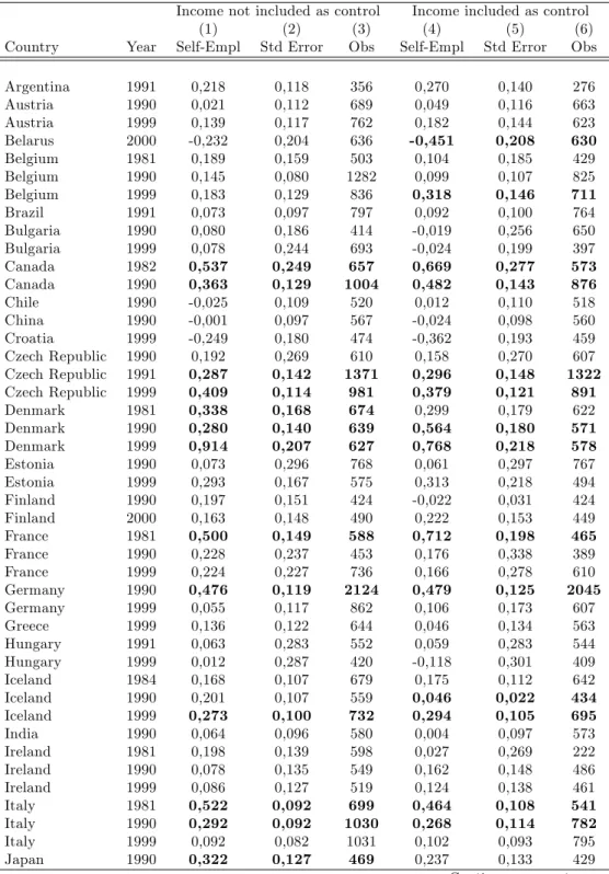
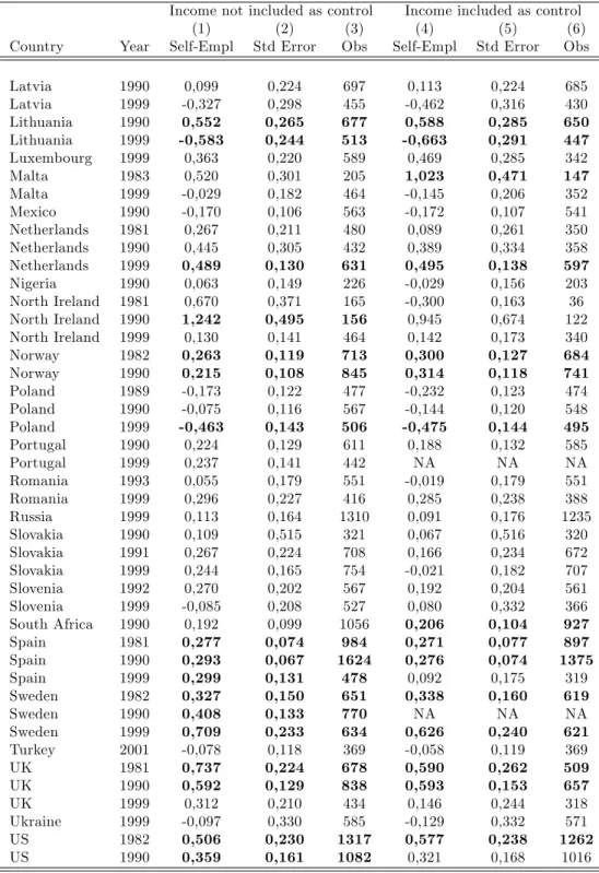
Table 2 reports the estimates of the coe¢ cient for each country and year. It is clear that the self-employed are not always more satis…ed than the employees, but this tends to be the case only in more developed countries. Moreover, the results remain basically unchanged if income is included in the set of controls Xi (columns 4-6). In fact, the set of countries and years in
which the self-employed enjoy higher utility becomes slightly larger, which already suggests that income di¤erentials are not the explanation behind di¤erences in job satisfaction.
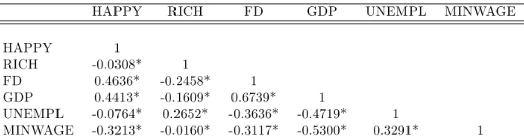
In order to better highlight these relationships, we construct the follow-ing variables. The variable HAP P Y is equal to the estimated coe¢ cient in equation (13), weighted by the inverse of its standard error. We also run a similar regression with income as dependent variable in equation (13). Given this regression, we construct the dummy RICH which is again equal to the estimated coe¢ cient weighted by the inverse of its standard error.16 As shown in Table 3, the variable HAP P Y is positively correlated with …nancial development, GDP per capita and it is negatively correlated with RICH; the level of unemployment (UNEMPL) and whether there is a mandatory minimum wage (MINWAGE): In accordance with our model, the self-employed enjoy higher utility than the employees in countries with high …nancial development and low labor market imperfections. Moreover, in these countries, the self-employed tend to have a lower income than the employees.
5.2 Job Satisfaction and Financial Development
The previous results suggest that utility di¤erences are not due to …nancial market imperfections. We now explore this argument more systematically. We …rst estimate the equation
Ui;c;t = + Xi;c;t+ Ic;t+ F Dc;t SEi;c;t+ "i;c;t; (14)
where Ui;c;t denotes the reported job satisfaction for an individual i in
coun-try c and year t; Xi;c;t is a set of individual variables including gender,
age, age-squared, education, marital status and employment status; Ic;tis a
country-year dummy, F Dc;tis the level …nancial development and SEi;c;t is
a dummy equal to one if i is self-employed; …nally, "i;c;t is the error term.17
Equation (14) follows the spirit of Rajan and Zingales (1998), and it allows to estimate the e¤ect of …nancial development on a particular set of individuals, the self-employed, after having controlled for the e¤ect on the
1 6
Our results are unchanged if instead we de…ne HAP P Y and RICH by considering only statistically signi…cant coe¢ cients.
1 7
Since these errors may re‡ect common components within countries and employment status groups, we cluster standard errors at the country/employment status level.
whole population and for country-year …xed e¤ects. Our main interest is in the coe¢ cient ; which describes how …nancial development a¤ects the job satisfaction of the self-employed relative to (full-time) employees.18 When is positive, we say that …nancial development is positively correlated with entrepreneurial utility.
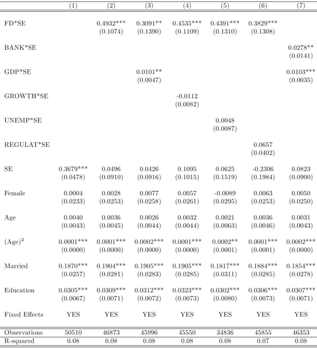
Table 4 reports our estimates on the full sample. The …rst column in-cludes only the controls Xi;c;t. Self-employed, old, married and well-educated
individuals tend to be more satis…ed with their jobs. The second column describes our most basic speci…cation, as reported in equation (14). The coe¢ cient is positive and statistically signi…cant. Financial development bene…ts the self-employed more than the employees.
In order to check the robustness of this result, we …rst try to identify whether …nancial development is capturing any e¤ect of better macroeco-nomic conditions, like better institutions or ecomacroeco-nomic perspectives, which may have a di¤erential impact on the self-employed. When we include GDP per capita, interacted with the employment status dummy, the e¤ect of …nancial development becomes slightly weaker, but still highly signi…cant (column 3). Adding other macroeconomic variables like GDP growth (col-umn 4), unemployment (col(col-umn 5), and an index of regulatory pressure (column 6), always interacted with the self-employment dummy, does not change the estimate of . Hence, our preferred speci…cation, which serves as the baseline for the next analysis, is the one in column (3).
We then check whether this pattern is con…rmed when using a variable based on the percentage of bank deposits held in privately owned banks (BANK), which is a measure of the development of the banking sector. This variable can be employed either as an instrument for …nancial develop-ment, as in Aghion et al. (2007) (see Table 5); or as an alternative measure of …nancial development (reduced form). The results in column 7 show that this measure of …nancial development is also positively correlated with entrepreneurial utility.
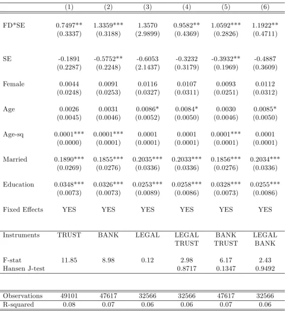
In addition, despite endogeneity may be less of a concern in our spec-i…cations, in that we estimate how a macro variable a¤ects an individual variable and we include country-year …xed e¤ects, we investigate whether our estimates may be biased, e.g. due to omitted variables, by using in-strumental variables. In line with the previous literature, we instrument …nancial development with legal origin (as in several papers, surveyed in Levine, 2005), with the level of trust (as in Guiso, Sapienza and Zingales, 2004) and, as already mentioned, with the variable BANK. While these
re-1 8
To facilitate the interpretation of our coe¢ cients, part-time employees and farmers are excluded from the analysis. These exclusions do not change our results. For the same reason, in what follows, we report the estimates from OLS regressions. The results using ordered probit are qualitatively the same (see Ferrer-i Carbonell and Frijters, 2004 for a methodological discussion). Finally, these results are robust to the use of di¤erent sampling weights.
sults should be interpreted with caution, due to well-known issues of …nding valid instruments for …nancial development, we nonetheless notice that they are consistent with the previous estimates (see Table 5).19
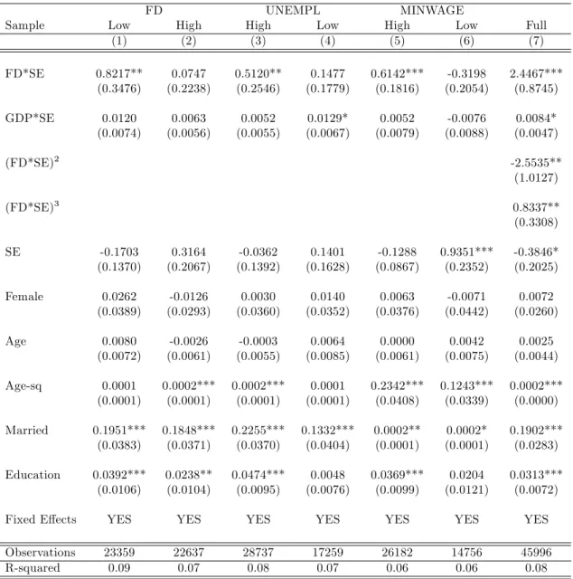
Our next set of regressions estimates whether the e¤ect of …nancial de-velopment depends on the country’s stage of dede-velopment. We divide the sample into country-years with high and with low …nancial development, where this threshold is determined by the median value in our sample.20 The results are in columns (1)-(2) of Table 6: the e¤ects of …nancial de-velopment on entrepreneurial utility are positive and signi…cant only in less developed countries.
Our model suggests a possible explanation for this result. In less de-veloped countries, individuals become self-employed either because of their motivation or for lack of salaried jobs. As these countries develop their …-nancial system, more jobs are created so only those who value it the most remain self-employed. This composition e¤ect is weaker in more developed countries, where labor demand is higher and so most individuals become self-employed by choice. Indeed, we get similar …ndings if we split the sam-ple according to unemployment (UNEMPL; columns 3-4) or to whether the country has a mandatory minimum wage (MINWAGE; columns 5-6). The e¤ect of …nancial development on entrepreneurial utility is stronger in coun-tries where unemployment is high and there is a minimum wage.21 Finally, to highlight the nonlinearity in the e¤ects of …nancial development, column (7) includes the level of …nancial development squared and cube. The …rst appears to be negative, the second positive, and both are signi…cant.
From these results, it is evident that the self-employed enjoy higher util-ity than the employees only in countries with high …nancial development; in less developed countries, entrepreneurial utility increases with …nancial development. In highly developed countries, approximately those above the sample median, the e¤ect of …nancial development is U-shaped, and it ap-pears not statistically signi…cant if one applies a linear model.
5.3 Mechanisms
We now explore the mechanisms underlying the relation between …nancial development and entrepreneurial utility. As stressed in our model, these mechanisms should not be evaluated only in monetary terms.
We start by enriching the set of regressors in equation (14). First, we control for income, both in the full sample and separating country-years
1 9The only di¤erence is that the e¤ect of …nancial development does not appear
statis-tically signi…cant when instrumented by the variable LEGAL alone. This is probably due to the poor …t of this variable in the …rst stage, as shown by the F-statistic.
2 0Splitting the sample according to the mean gives the same qualitative results. 2 1
Similarly, we …nd that the e¤ects are stronger when GDP per capita is low and labor market regulation (as described by the variable LABOR) is high.
according to their level of …nancial development. As shown in columns (1)-(3) of Table 7, if anything, the results are even stronger. Income appears to be a major determinant of job satisfaction; but, as Benz and Frey (2004) have also observed, higher income does not explain entrepreneurial utility. In addition to the existing literature, we document that the e¤ects of …nancial development on entrepreneurial utility are not only monetary.22
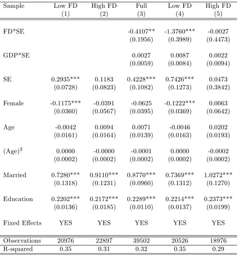
To get further evidence along these lines, we estimate equation (14) with income as dependent variable. Results appear in Table 8. We observe that the self-employed are richer than the employees in less developed countries, while this is not the case in more developed countries (columns 1-2). More-over, …nancial development decreases the income of the self-employed, rela-tive to the income of the employees (column 3), and this e¤ect tends to be stronger in less developed countries (columns 4-5). The fact that …nancial development reduces pro…ts is consistent with our model in that …nancial development increases competition, either in the product or in the labor market.
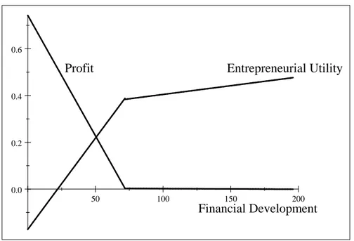
The results in columns (4)-(5) of Table 8 and those in columns (1)-(2) of Table 6 are used to draw Figure 1, which summarizes our main results so far. It clearly emerges that the e¤ects of …nancial development on entrepreneurial utility may di¤er from those on pro…t; actually, in our case, these e¤ects go exactly in the opposite direction. Entrepreneurial utility increases with …nancial development, while pro…t decreases. Moreover, both e¤ects tend to be stronger in less developed countries.
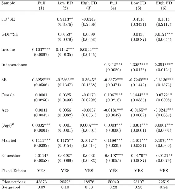
The above results suggest that …nancial development works through non-monetary aspects of job satisfaction. To better identify these mechanisms, we include in our regressions variables such as the degree of pride in one’s work, the satisfaction with job security and the degree of independence enjoyed in the job. We also control for work-related beliefs such as how important work is in one’s life, the main reason why one works, and so on. None of these variables signi…cantly a¤ects our results, with the exception of independence, which is an indicator derived from the question: "How free are you to make decisions in your job?" The importance of this variable in explaining entrepreneurial utility has already been pointed out in Benz and Frey (2004), and indeed, also in our sample, being self-employed becomes negatively related to job satisfaction when we add this control (Table 7, column 4).
We observe that, once independence has been controlled for, the e¤ect of …nancial development almost halves in magnitude and is not statistically signi…cant (column 5). Hence, our results add to the existing evidence by documenting that most of the e¤ects of …nancial development seem to work
2 2Note that while income under-reporting may be more of an issue for the self-employed,
this could only explain our results if under-reporting was higher in more …nancially devel-oped countries.
50 100 150 200 0.0
0.2 0.4 0.6
Profit
Entrepreneurial Utility
Financial Development
Figure 1: Entrepreneurial Pro…t, Utility and Financial Development.
Estimates from Table 6, Columns (1)-(2) and Table 8, Columns (4)-(5).
through this channel. According to the model, this is the case because …nancial development o¤ers to the most motivated individuals the opportu-nity to become entrepreneurs. Indeed, these results suggest that what we have so far called motivation may be (broadly) de…ned in terms of taste for independence at work. Moreover, the coe¢ cient on independence in less developed countries is lower than in more developed countries (columns 5 and 6).23 This suggests that, as in our model, in more developed countries independence is given to those who value it the most.
6
Conclusion and Policy Implications
We started our analysis by examining the argument that entrepreneurs en-joy higher utility than employees due to a lack of …nancial development. This argument has not found support in our data; on the contrary, we have shown that …nancial development increases utility di¤erences between the self-employed and employees. Moreover, this e¤ect is not explained by in-creased pro…ts; rather, it seems to work through non-monetary dimensions of job satisfaction, and in particular independence. We have interpreted these …ndings by building a simple occupational choice model in which …-nancial development favors both job creation and a better matching between
2 3
individual motivation and occupation.
According to our results, the existence of utility di¤erences is not due to some market imperfection, and as such it does not in itself call for policy intervention. By highlighting how …nancial development a¤ects also non-monetary dimensions of entrepreneurial utility, instead, the results point toward other policy implications. First, they bring an additional reason to promote an e¢ cient …nancial system. Second, from the viewpoint of promoting entrepreneurship, they suggest that recognizing the importance of entrepreneurs’intrinsic motivation does not imply that external conditions do not matter. It then appears that a broader investigation on how di¤erent markets and institutions a¤ect non-monetary returns from a job would be of great interest both for researchers and policy makers.
References
Addison, J. T. and Teixeira, P. (2003), ‘The economics of employment pro-tection’, Journal of Labor Research 24(1), 85–129.
Aghion, P., Fally, T. and Scarpetta, S. (2007), ‘Credit constraints as a barrier to the entry and post-entry growth of …rms’, Economic Pol-icy 22(52), 731–779.
Andersson, P. and Wadensjö, E. (2007), ‘Do the unemployed become suc-cessful entrepreneurs? a comparison between the unemployed, inactive and wage-earners’, International Journal of Manpower 28, 604–626. Banerjee, A. V. and Du‡o, E. (2005), Growth theory through the lens of
development economics, in P. Aghion and S. Durlauf, eds, ‘Handbook of Economic Growth’, Vol. 1 of Handbook of Economic Growth, Elsevier, chapter 7, pp. 473–552.
Banerjee, A. V. and Du‡o, E. (2008), ‘What is middle class about the middle classes around the world?’, Journal of Economic Perspectives 22(2), 3– 28.
Banerjee, A. V. and Newman, A. F. (1993), ‘Occupational choice and the process of development’, Journal of Political Economy 101(2), 274–98. Benz, M. and Frey, B. S. (2004), ‘Being independent raises happiness at
work’, Swedish Economic Policy Review 11, 95–134.
Berner, E., Gomez, G. and Knorringa, P. (2008), ‘Helping a Large Number of People Become a Little Less Poor: The Logic of Survival Entrepre-neurs’, Mimeo. ISS, The Hague.
Bianchi, M. and Henrekson, M. (2005), ‘Is neoclassical economics still en-trepreneurless?’, Kyklos 58(3), 353–377.
Blanch‡ower, D. G. and Oswald, A. J. (1998), ‘What makes an entrepre-neur?’, Journal of Labor Economics 16(1), 26–60.
Blanch‡ower, D. G., Oswald, A. and Stutzer, A. (2001), ‘Latent entrepre-neurship across nations’, European Economic Review 45(4-6), 680–691. Borjas, G. J. (1986), ‘The self-employment experience of immigrants’,
Jour-nal of Human Resources 21(4), 485–506.
Botero, J., Djankov, S., La Porta, R. and Lopez-De-Silanes, F. C. (2004), ‘The regulation of labor’, Quarterly Journal of Economics 119(4), 1339–1382.
Congregado, E., Golpe, A. A. and Parker, S. C. (2009), ‘The dynamics of entrepreneurship: Hysteresis, business cycles and government policy’, IZA Discussion Paper No. 4093.
Constant, A. and Zimmermann, K. F. (2004), ‘Self-employment dynamics across the business cycle: Migrants versus natives’, IZA Discussion Paper No. 1386.
Evans, D. S. and Leighton, L. S. (1989), ‘Some empirical aspects of entre-preneurship’, American Economic Review 79(3), 519–35.
Ferrer-i Carbonell, A. and Frijters, P. (2004), ‘How important is method-ology for the estimates of the determinants of happiness?’, Economic Journal 114(497), 641–659.
Fuchs-Schündeln, N. (2009), ‘On preferences for being self-employed’, Jour-nal of Economic Behavior and Organization 71(2), 162–171.
Glocker, D. and Steiner, V. (2007), ‘Self-employment: A way to end unem-ployment? empirical evidence from german pseudo-panel data’, IZA Discussion Paper No. 2561.
Guiso, L., Sapienza, P. and Zingales, L. (2004), ‘Does Local Financial De-velopment Matter?’, Quarterly Journal of Economics 119(3), 929–969. Hamilton, B. H. (2000), ‘Does entrepreneurship pay? an empirical analy-sis of the returns to self-employment’, Journal of Political Economy 108(3), 604–631.
Harris, J. R. and Todaro, M. P. (1970), ‘Migration, unemployment & development: A two-sector analysis’, American Economic Review 60(1), 126–42.
Holmes, T. J. and Schmitz, James A, J. (1990), ‘A theory of entrepreneur-ship and its application to the study of business transfers’, Journal of Political Economy 98(2), 265–94.
Holmstrom, B. and Tirole, J. (1997), ‘Financial intermediation, loan-able funds, and the real sector’, Quarterly Journal of Economics 112(3), 663–91.
Hundley, G. (2001), ‘Why and when are the self-employed more satis…ed with their work?’, Industrial Relations 40(2), 293–316.
Kerr, W. R. and Nanda, R. (2009), ‘Financing constraints and entrepreneur-ship’, NBER Working Paper No. 15498.
Kihlstrom, R. E. and La¤ont, J.-J. (1979), ‘A general equilibrium entre-preneurial theory of …rm formation based on risk aversion’, Journal of Political Economy 87(4), 719–48.
Knight, F. (1921), Risk, Uncertainty and Pro…t, New York: Houghton Mif-‡in.
La Porta, R., Lopez-de Silanes, F., Shleifer, A. and Vishny, R. (1998), ‘Law and Finance’, Journal of Political Economy 106(6), 1113–1155. Levine, R. (2005), Finance and growth: Theory and evidence, in P. Aghion
and S. Durlauf, eds, ‘Handbook of Economic Growth’, Vol. 1 of Hand-book of Economic Growth, Elsevier, chapter 12, pp. 865–934.
Loayza, N. V. (1994), ‘Labor regulations and the informal economy’, The World Bank Policy Research Working Paper No. 1335.
Lucas, R. E. J. (1978), ‘On the size distribution of business …rms’, Bell Journal of Economics 9(2), 508–523.
Mandelman, F. S. and Rojas, G. V. M. (2007), ‘Microentrepreneurship and the business cycle: is self-employment a desired outcome?’, Federal Reserve Bank of Atlanta Working Paper No. 2007-15.
Moskowitz, T. J. and Vissing-Jorgensen, A. (2002), ‘The returns to entre-preneurial investment: A private equity premium puzzle?’, American Economic Review 92(4), 745–778.
Parker, S. (2004), The Economics of Self-Employment and Entrepreneur-ship, Cambridge University Press.
Rajan, R. G. and Zingales, L. (1998), ‘Financial dependence and growth’, American Economic Review 88(3), 559–86.
Reynolds, P., Bygrave, W., Autio, E., Cox, L. and Hay, M. (2002), Global Entrepreneurship Monitor: 2002 executive report, Babson College. Schneider, F. and Enste, D. H. (2000), ‘Shadow economies: Size, causes,
and consequences’, Journal of Economic Literature 38(1), 77–114. Schumpeter, J. A. (1934), The Theory of Economic Development,
Cam-bridge, MA: Harvard University Press.
Shapiro, C. and Stiglitz, J. E. (1984), ‘Equilibrium unemployment as a worker discipline device’, American Economic Review 74(3), 433–44. Stel, A., Carree, M. and Thurik, R. (2005), ‘The E¤ect of Entrepreneurial
Activity on National Economic Growth’, Small Business Economics 24(3), 311–321.
Taylor, M. P. (1996), ‘Earnings, independence or unemployment: Why become self-employed?’, Oxford Bulletin of Economics and Statistics 58(2), 253–66.
van Praag, C. M. and Versloot, P. H. (2007), ‘What is the value of entre-preneurship? a review of recent research’, IZA Discussion Paper No. 3014.
Weiss, A. W. (1980), ‘Job queues and layo¤s in labor markets with ‡exible wages’, Journal of Political Economy 88(3), 526–38.
Wennekers, S. and Thurik, R. (1999), ‘Linking Entrepreneurship and Eco-nomic Growth’, Small Business EcoEco-nomics 13(1), 27–56.
7
Appendix
7.1 Omitted Proofs
Lemma 1 The minimal entrepreneurial motivation b is increasing with the share of entrepreneurs x1.
Proof. With simple algebra, di¤erentiating equation (7), one can write @b @x1 = wl (1 x1)2 @p @x1 q:
This expression is positive since the …rst term is positive (note that x1 may
increase only if lx1+ x1 < 1; i.e. there is excess labor supply and w = w,
which implies that w does not depend directly on x1) and the second term
is negative (Q increases in x1 and so p decreases in x1):
Lemma 2 There exists a level of …nancial development c such that the share of entrepreneurs x1 increases in c for c < c and it is x1= 1=(1+l)
for all c c :
Proof. Suppose …rst that lx1+ x1< 1; i.e. there is excess labor supply
and w = w: Implicitly di¤erentiating equation (8), we have @x1 @c = f (a )[1 G(b )] 1 + [1 F (a )]g(b )@x@b 1 :
The numerator measures the increment in individuals who can a¤ord to be-come entrepreneurs. The denominator indicates how the mass of individuals who are su¢ ciently motivated and so willing to be entrepreneurs changes as entry increases. Given Lemma 1, @b =@x1 is positive and hence @x1=@c is
also positive. Hence, x1 is strictly increasing in c for lx1+ x1 < 1: Let c be
the minimal c such that x1 = 1=(1 + l): Beyond c ; x1 cannot increase any
further since everyone is employed either as a worker or as an entrepreneur.
Lemma 3 For c < c ; the price p decreases with c and the wage w is constant at w; for c c ; the price p is constant and the wage w increases with c.
Proof. Given Lemma 2, x1 is strictly increasing in c for c < c : The
total output produced Q = x1q depends positively on x1 hence for equation
(4) the price p decreases with x1: The wage w instead does not depend on
x1; since x1 can increase only if there is excess labor supply and so w = w:
supply of labor, i.e. L = 1 x1 lx1 0: Implicitly di¤erentiating L, we have @w @c = @L @c= @L @w = f (a )[1 G(b )] [1 F (a )]g(b )(1 + l) > 0: Proposition 2
a. Entrepreneurs enjoy higher utility than employees only in more …nan-cially developed countries.
b. Entrepreneurial pro…ts decrease with …nancial development.
c. Entrepreneurial non-monetary bene…ts b increase with …nancial develop-ment, and this e¤ ect may be stronger when …nancial development is low.
Proof. Recall from equation (12) that
U1
lx1
1 x1
U2:
If c is low, then x1 is low and so there are many entrepreneurs for which
U1 < U2: These are the individuals with motivation b 2 [b ; b ]; where b
is such that + b = w: If c c ; then lx1 = 1 x1 and U1 U2 for
all entrepreneurs. Part b. of the Proposition follows from Lemma 3: as c increases, either p decreases or w increases, hence the pro…t = pq wl k decreases with c. Finally, from equation (9), we have
@b @c = g(b ) 1 G(b )(b b ) @b @c:
From equation (7), we see that b increases in x1 and p and it decreases in w
so, given Lemmas 1, 2 and 3, @b =@c > 0. This implies that b increases in c: Notice also that this e¤ect may be stronger for c < c ; when b increases in c both as the result of reduced pro…t and of an higher probability of being hired (an higher lx1=(1 x1)). For c c ; instead, only the …rst e¤ect is at
7.2 Description of variables
Individual variables:
Job Satisfaction: 1-10 index based on the answer to "Overall, how sat-is…ed or dissatsat-is…ed are you with your job?" 10 indicates "satsat-is…ed", 1 indi-cates "dissatis…ed". Source: WVS, variable c033.
SE: Dummy equal 1 if the individual is self-employed. Source: WVS, variable x028.
Female: Dummy equal 1 if the individual is a female. Source: WVS, variable x001.
Age: Age of the individual. Source: WVS, variable x003.
Married: Dummy equal 1 if the individual is married or living together as married. Source: WVS, variable x007.
Education: 1-10 index for the age at which the individual completed education. 1 indicates the individual was less than 13 years old, 10 indicates the individual was more than 20 years old. Source: WVS, variable x023r.
Income: 1-11 index of the individual income scale. Source: WVS, vari-able x047.
Independence in job: 1-10 index based on the answer to "How free are you to make decisions in your job?" 10 indicates "a great deal", 1 indicates "none at all". Source: WVS, variable c034.
Macro variables:
FD: Financial Development, measured by the level of domestic credit to the private sector (% of GDP). Source: World Development Indicators. (available at www.worldbank.org/data)
GDP: GDP per capita (at constant 2000 US$). Source: World Develop-ment Indicators. (available at www.worldbank.org/data)
UNEMPL: Total unemployment (% of total labor force). Source: World Development Indicators. (available at www.worldbank.org/data)
MINWAGE: Dummy equal 1 if the country has a mandatory minimum wage de…ned by statute or there is a minimum wage established by manda-tory collective agreement which is legally binding for most sectors of the
economy. The variable is a cross county taken in 1997. Source: Botero, Djankov, La Porta and Lopez-De-Silanes (2004).
LABOR: 0-10 variable rating the regulation of labor markets. 0 corre-sponds to stronger state intervention. Source: Economic Freedom of the World: 2007 Annual Report. (available at www.freetheworld.com)
REGULAT: 0-10 variable rating the regulation of credit markets, la-bor markets and businesses. 0 corresponds to stronger state intervention. Source: Economic Freedom of the World: 2007 Annual Report. (available at www.freetheworld.com)
GROWTH: GDP per capita growth (annual %). Source: World Devel-opment Indicators. (available at www.worldbank.org/data)
BANK: 0-10 variable based on the percentage of bank deposits held in privately owned banks. Countries with larger shares of privately held deposits received higher ratings. Source: Economic Freedom of the World: 2007 Annual Report. (available at www.freetheworld.com)
TRUST: Average response to the question "Generally speaking, would you say that most people can be trusted? " 1 indicates that "most people can be trusted", 0 indicates "Can’t be too careful in dealing with people". Source: WVS, variable a165.
LEGAL: Dummy equal 1 if the country’s legal origin is civil law. Source: La Porta, Lopez-de Silanes, Shleifer and Vishny (1998).
7.3 Tables
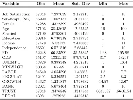
Table 1: Summary statistics
Variable Obs Mean Std. Dev Min Max
Job Satisfaction 67348 7.297039 2.182215 1 10 Self-Empl. (SE) 65999 .1062137 .3081133 0 1 Female 67288 .4372399 .4960492 0 1 Age 67193 38.48615 12.25545 16 100 Married 67100 .6798361 .4665429 0 1 Education 60816 6.730318 2.719934 1 10 Income 57479 5.53122 2.410663 1 11 Independence 66691 6.571516 2.68442 1 10 FD 62248 66.83599 38.53845 1.68 195.98 GDP 65197 13311.15 9797.721 317 43267 UNEMPL 43829 8.398348 4.252513 .6 16.4 MINWAGE 60068 .65589 .4750811 0 1 LABOR 54640 4.654596 1.43885 1.8 7.7 REGULAT 62491 5.326551 1.204252 2.5 8.3 GROWTH 64627 1.231817 4.798632 -14.57 12.67 BANK 62021 5.678464 3.725851 0 10 TRUST 67348 .3476848 .1347544 .0645527 .6646154 LEGAL 43981 .727928 .4450318 0 1
Note: The table reports summary statistics for all variables used in the regressions. A de…nition of these variables can be found in Section 7.2.
Table 2: Job Satisfaction across countries
Income not included as control Income included as control (1) (2) (3) (4) (5) (6) Country Year Self-Empl Std Error Obs Self-Empl Std Error Obs
Argentina 1991 0,218 0,118 356 0,270 0,140 276 Austria 1990 0,021 0,112 689 0,049 0,116 663 Austria 1999 0,139 0,117 762 0,182 0,144 623 Belarus 2000 -0,232 0,204 636 -0,451 0,208 630 Belgium 1981 0,189 0,159 503 0,104 0,185 429 Belgium 1990 0,145 0,080 1282 0,099 0,107 825 Belgium 1999 0,183 0,129 836 0,318 0,146 711 Brazil 1991 0,073 0,097 797 0,092 0,100 764 Bulgaria 1990 0,080 0,186 414 -0,019 0,256 650 Bulgaria 1999 0,078 0,244 693 -0,024 0,199 397 Canada 1982 0,537 0,249 657 0,669 0,277 573 Canada 1990 0,363 0,129 1004 0,482 0,143 876 Chile 1990 -0,025 0,109 520 0,012 0,110 518 China 1990 -0,001 0,097 567 -0,024 0,098 560 Croatia 1999 -0,249 0,180 474 -0,362 0,193 459 Czech Republic 1990 0,192 0,269 610 0,158 0,270 607 Czech Republic 1991 0,287 0,142 1371 0,296 0,148 1322 Czech Republic 1999 0,409 0,114 981 0,379 0,121 891 Denmark 1981 0,338 0,168 674 0,299 0,179 622 Denmark 1990 0,280 0,140 639 0,564 0,180 571 Denmark 1999 0,914 0,207 627 0,768 0,218 578 Estonia 1990 0,073 0,296 768 0,061 0,297 767 Estonia 1999 0,293 0,167 575 0,313 0,218 494 Finland 1990 0,197 0,151 424 -0,022 0,031 424 Finland 2000 0,163 0,148 490 0,222 0,153 449 France 1981 0,500 0,149 588 0,712 0,198 465 France 1990 0,228 0,237 453 0,176 0,338 389 France 1999 0,224 0,227 736 0,166 0,278 610 Germany 1990 0,476 0,119 2124 0,479 0,125 2045 Germany 1999 0,055 0,117 862 0,106 0,173 607 Greece 1999 0,136 0,122 644 0,046 0,134 563 Hungary 1991 0,063 0,283 552 0,059 0,283 544 Hungary 1999 0,012 0,287 420 -0,118 0,301 409 Iceland 1984 0,168 0,107 679 0,175 0,112 642 Iceland 1990 0,201 0,107 559 0,046 0,022 434 Iceland 1999 0,273 0,100 732 0,294 0,105 695 India 1990 0,064 0,096 580 0,004 0,097 573 Ireland 1981 0,198 0,139 598 0,027 0,269 222 Ireland 1990 0,078 0,135 549 0,162 0,148 486 Ireland 1999 0,086 0,127 519 0,124 0,138 461 Italy 1981 0,522 0,092 699 0,464 0,108 541 Italy 1990 0,292 0,092 1030 0,268 0,114 782 Italy 1999 0,092 0,082 1031 0,102 0,093 795 Japan 1990 0,322 0,127 469 0,237 0,133 429 Continues on next page
Table 2 continued
Income not included as control Income included as control (1) (2) (3) (4) (5) (6) Country Year Self-Empl Std Error Obs Self-Empl Std Error Obs
Latvia 1990 0,099 0,224 697 0,113 0,224 685 Latvia 1999 -0,327 0,298 455 -0,462 0,316 430 Lithuania 1990 0,552 0,265 677 0,588 0,285 650 Lithuania 1999 -0,583 0,244 513 -0,663 0,291 447 Luxembourg 1999 0,363 0,220 589 0,469 0,285 342 Malta 1983 0,520 0,301 205 1,023 0,471 147 Malta 1999 -0,029 0,182 464 -0,145 0,206 352 Mexico 1990 -0,170 0,106 563 -0,172 0,107 541 Netherlands 1981 0,267 0,211 480 0,089 0,261 350 Netherlands 1990 0,445 0,305 432 0,389 0,334 358 Netherlands 1999 0,489 0,130 631 0,495 0,138 597 Nigeria 1990 0,063 0,149 226 -0,029 0,156 203 North Ireland 1981 0,670 0,371 165 -0,300 0,163 36 North Ireland 1990 1,242 0,495 156 0,945 0,674 122 North Ireland 1999 0,130 0,141 464 0,142 0,173 340 Norway 1982 0,263 0,119 713 0,300 0,127 684 Norway 1990 0,215 0,108 845 0,314 0,118 741 Poland 1989 -0,173 0,122 477 -0,232 0,123 474 Poland 1990 -0,075 0,116 567 -0,144 0,120 548 Poland 1999 -0,463 0,143 506 -0,475 0,144 495 Portugal 1990 0,224 0,129 611 0,188 0,132 585 Portugal 1999 0,237 0,141 442 NA NA NA Romania 1993 0,055 0,179 551 -0,019 0,179 551 Romania 1999 0,296 0,227 416 0,285 0,238 388 Russia 1999 0,113 0,164 1310 0,091 0,176 1235 Slovakia 1990 0,109 0,515 321 0,067 0,516 320 Slovakia 1991 0,267 0,224 708 0,166 0,234 672 Slovakia 1999 0,244 0,165 754 -0,021 0,182 707 Slovenia 1992 0,270 0,202 567 0,192 0,204 561 Slovenia 1999 -0,085 0,208 527 0,080 0,332 366 South Africa 1990 0,192 0,099 1056 0,206 0,104 927 Spain 1981 0,277 0,074 984 0,271 0,077 897 Spain 1990 0,293 0,067 1624 0,276 0,074 1375 Spain 1999 0,299 0,131 478 0,092 0,175 319 Sweden 1982 0,327 0,150 651 0,338 0,160 619 Sweden 1990 0,408 0,133 770 NA NA NA Sweden 1999 0,709 0,233 634 0,626 0,240 621 Turkey 2001 -0,078 0,118 369 -0,058 0,119 369 UK 1981 0,737 0,224 678 0,590 0,262 509 UK 1990 0,592 0,129 838 0,593 0,153 657 UK 1999 0,312 0,210 434 0,146 0,244 318 Ukraine 1999 -0,097 0,330 585 -0,129 0,332 571 US 1982 0,506 0,230 1317 0,577 0,238 1262 US 1990 0,359 0,161 1082 0,321 0,168 1016
Note: This table reports the results of ordered probit regressions of job satisfaction on a dummy equal 1 if the individual is self-employed. Columns (1) and (4) report the estimated coe¢ cients. In columns (1)-(3), the controls are gender, age, age squared, education, marital status. In columns (4)-(6), income is also included in the controls.
Table 3: Partial correlations
HAPPY RICH FD GDP UNEMPL MINWAGE
HAPPY 1 RICH -0.0308* 1 FD 0.4636* -0.2458* 1 GDP 0.4413* -0.1609* 0.6739* 1 UNEMPL -0.0764* 0.2652* -0.3636* -0.4719* 1 MINWAGE -0.3213* -0.0160* -0.3117* -0.5300* 0.3291* 1 Note: The table reports partial correlation coe¢ cients. The star indicates sig-ni…cance at the 1% level. HAPPY is equal to the estimated coe¢ cient on self-employment, weighted by the inverse of its standard error, in an ordered probit regression with job satisfaction as dependent variable. RICH is equal to the esti-mated coe¢ cient on self-employment, weighted by the inverse of its standard error, in an ordered probit regression with income as dependent variable. All regressions include gender, age, age squared, education, marital status as controls.
Table 4: Financial Development and Job Satisfaction: Basic results (1) (2) (3) (4) (5) (6) (7) FD*SE 0.4932*** 0.3091** 0.4535*** 0.4391*** 0.3829*** (0.1074) (0.1390) (0.1109) (0.1310) (0.1308) BANK*SE 0.0278** (0.0141) GDP*SE 0.0101** 0.0103*** (0.0047) (0.0035) GROWTH*SE -0.0112 (0.0082) UNEMP*SE 0.0048 (0.0087) REGULAT*SE 0.0657 (0.0402) SE 0.3679*** 0.0496 0.0426 0.1095 0.0625 -0.2306 0.0823 (0.0478) (0.0910) (0.0916) (0.1015) (0.1519) (0.1984) (0.0900) Female 0.0004 0.0028 0.0077 0.0057 -0.0089 0.0063 0.0050 (0.0233) (0.0253) (0.0258) (0.0261) (0.0295) (0.0253) (0.0250) Age 0.0040 0.0036 0.0026 0.0032 0.0021 0.0036 0.0031 (0.0043) (0.0045) (0.0044) (0.0044) (0.0063) (0.0046) (0.0043) (Age)2 0.0001*** 0.0001*** 0.0002*** 0.0001*** 0.0002** 0.0001*** 0.0002*** (0.0000) (0.0000) (0.0000) (0.0000) (0.0001) (0.0001) (0.0000) Married 0.1870*** 0.1904*** 0.1905*** 0.1905*** 0.1817*** 0.1884*** 0.1854*** (0.0257) (0.0281) (0.0283) (0.0285) (0.0311) (0.0285) (0.0278) Education 0.0305*** 0.0309*** 0.0312*** 0.0323*** 0.0302*** 0.0306*** 0.0307*** (0.0067) (0.0071) (0.0072) (0.0073) (0.0080) (0.0073) (0.0071)
Fixed E¤ects YES YES YES YES YES YES YES
Observations 50510 46873 45996 45550 34836 45855 46353 R-squared 0.08 0.08 0.08 0.08 0.08 0.07 0.08
Note: This table reports the results of OLS regressions with job satisfaction as dependent variable. All regressions include country-year dummies. The coe¢ cient estimates and the standard errors for FD*SE are multiplied by 100. The coe¢ cient estimates and the standard errors for GDP*SE are multiplied by 1000. Robust standard errors, clustered at the country-employment status level, are in brackets. , and denote rejection of the null hypothesis of the coe¢ cient being equal to 0 at 10%, 5% and 1% signi…cance level, respectively.
Table 5: Financial Development and Job Satisfaction: Instrumental variables (1) (2) (3) (4) (5) (6) FD*SE 0.7497** 1.3359*** 1.3570 0.9582** 1.0592*** 1.1922** (0.3337) (0.3188) (2.9899) (0.4369) (0.2826) (0.4711) SE -0.1891 -0.5752** -0.6053 -0.3232 -0.3932** -0.4887 (0.2287) (0.2248) (2.1437) (0.3179) (0.1969) (0.3609) Female 0.0044 0.0091 0.0116 0.0107 0.0093 0.0112 (0.0248) (0.0253) (0.0327) (0.0311) (0.0251) (0.0312) Age 0.0026 0.0031 0.0086* 0.0084* 0.0030 0.0085* (0.0045) (0.0046) (0.0052) (0.0050) (0.0046) (0.0050) Age-sq 0.0001*** 0.0001*** 0.0001 0.0001 0.0001*** 0.0001 (0.0000) (0.0001) (0.0001) (0.0001) (0.0001) (0.0001) Married 0.1890*** 0.1855*** 0.2035*** 0.2033*** 0.1856*** 0.2034*** (0.0269) (0.0276) (0.0336) (0.0336) (0.0276) (0.0336) Education 0.0348*** 0.0326*** 0.0253*** 0.0258*** 0.0328*** 0.0255*** (0.0073) (0.0073) (0.0089) (0.0086) (0.0073) (0.0086)
Fixed E¤ects YES YES YES YES YES YES
Instruments TRUST BANK LEGAL LEGAL BANK LEGAL TRUST TRUST BANK
F-stat 11.85 8.98 0.12 2.98 6.17 2.43 Hansen J-test 0.8717 0.1347 0.9492
Observations 49101 47617 32566 32566 47617 32566 R-squared 0.08 0.07 0.06 0.06 0.07 0.06
Note: This table reports the results of IV regressions with job satisfaction as dependent variable. All regressions include country-year dummies. The coe¢ cient estimates and the standard errors for FD*SE are multiplied by 100. The F-statistic refers to the null hypothesis that the coe¢ cient of the excluded instrument is equal to zero in the …rst stage. Hansen J-test reports the p-values of Hansen overidenti…cation test, under the null hypothesis that the instruments are valid. Robust standard errors, clustered at the country-employment status level, are in brackets. , and denote rejection of the null hypothesis of the coe¢ cient being equal to 0 at 10%, 5% and 1% signi…cance level, respectively.
Table 6: Financial Development and Job Satisfaction: Non-linear e¤ects
FD UNEMPL MINWAGE
Sample Low High High Low High Low Full (1) (2) (3) (4) (5) (6) (7) FD*SE 0.8217** 0.0747 0.5120** 0.1477 0.6142*** -0.3198 2.4467*** (0.3476) (0.2238) (0.2546) (0.1779) (0.1816) (0.2054) (0.8745) GDP*SE 0.0120 0.0063 0.0052 0.0129* 0.0052 -0.0076 0.0084* (0.0074) (0.0056) (0.0055) (0.0067) (0.0079) (0.0088) (0.0047) (FD*SE)2 -2.5535** (1.0127) (FD*SE)3 0.8337** (0.3308) SE -0.1703 0.3164 -0.0362 0.1401 -0.1288 0.9351*** -0.3846* (0.1370) (0.2067) (0.1392) (0.1628) (0.0867) (0.2352) (0.2025) Female 0.0262 -0.0126 0.0030 0.0140 0.0063 -0.0071 0.0072 (0.0389) (0.0293) (0.0360) (0.0352) (0.0376) (0.0442) (0.0260) Age 0.0080 -0.0026 -0.0003 0.0064 0.0000 0.0042 0.0025 (0.0072) (0.0061) (0.0055) (0.0085) (0.0061) (0.0075) (0.0044) Age-sq 0.0001 0.0002*** 0.0002*** 0.0001 0.2342*** 0.1243*** 0.0002*** (0.0001) (0.0001) (0.0001) (0.0001) (0.0408) (0.0339) (0.0000) Married 0.1951*** 0.1848*** 0.2255*** 0.1332*** 0.0002** 0.0002* 0.1902*** (0.0383) (0.0371) (0.0370) (0.0404) (0.0001) (0.0001) (0.0283) Education 0.0392*** 0.0238** 0.0474*** 0.0048 0.0369*** 0.0204 0.0313*** (0.0106) (0.0104) (0.0095) (0.0076) (0.0099) (0.0121) (0.0072)
Fixed E¤ects YES YES YES YES YES YES YES
Observations 23359 22637 28737 17259 26182 14756 45996 R-squared 0.09 0.07 0.08 0.07 0.06 0.06 0.08
Note: This table reports the results of OLS regressions with job satisfaction as dependent variable. All regressions include country-year dummies. In columns (1)-(2), Low FD and High FD indicate that the sample is restricted to countries respectively below and above the median value of FD in our sample (equal to 71.78). Similarly, in columns (3)-(4), High UNEMPL and Low UNEMPL indicate that the sample is restricted to countries respectively above and below the median value of UNEMPL in our sample (equal to 8.2); and in columns (5)-(6), High MINWAGE and Low MINWAGE indicate that the sample is restricted to countries respectively with and without a mandatory minimum wage. The coe¢ cient estimates and the standard errors for FD*SE are multiplied by 100. The coe¢ cient estimates and the standard errors for GDP*SE are multiplied by 1000. Robust standard errors, clustered at the country-employment status level, are in brackets. , and denote rejection of the null hypothesis of the coe¢ cient being equal to 0 at 10%, 5% and 1% signi…cance level, respectively.
Table 7: Financial Development and Job Satisfaction: Mechanisms
Sample Full Low FD High FD Full Low FD High FD
(1) (2) (3) (4) (5) (6) FD*SE 0.9113** -0.0249 0.4510 0.1818 (0.3576) (0.2366) (0.3431) (0.2117) GDP*SE 0.0153* 0.0090 0.0136 0.0124*** (0.0079) (0.0058) (0.0087) (0.0045) Income 0.1037*** 0.1142*** 0.0944*** (0.0097) (0.0135) (0.0145) Independence 0.3418*** 0.3287*** 0.3513*** (0.0089) (0.0123) (0.0124) SE 0.3259*** -0.2866** 0.3645* -0.3372*** -0.7240*** -0.6136*** (0.0506) (0.1347) (0.1858) (0.0471) (0.1442) (0.1873) Female 0.0001 0.0325 -0.0170 0.1067*** 0.1444*** 0.0772** (0.0250) (0.0433) (0.0292) (0.0216) (0.0336) (0.0308) Age 0.0031 0.0056 -0.0037 -0.0181*** -0.0155** -0.0241*** (0.0045) (0.0082) (0.0061) (0.0042) (0.0062) (0.0067) (Age)2 0.0002*** 0.0001 0.0002*** 0.0003*** 0.0003*** 0.0004*** (0.0001) (0.0001) (0.0001) (0.0000) (0.0001) (0.0001) Married 0.1111*** 0.1175** 0.1012** 0.1186*** 0.1409*** 0.1070*** (0.0292) (0.0454) (0.0414) (0.0239) (0.0331) (0.0360) Education 0.0114* 0.0198* 0.0036 -0.0197*** -0.0179** -0.0181** (0.0058) (0.0099) (0.0083) (0.0055) (0.0087) (0.0079)
Fixed E¤ects YES YES YES YES YES YES
Observations 43873 20526 18976 50049 23107 22519 R-squared 0.09 0.10 0.08 0.23 0.23 0.24
Note: This table reports the results of OLS regressions with job satisfaction as dependent variable. All regressions include country-year dummies. Low FD and High FD indicate that the sample is restricted to countries respectively below and above the median value of FD in our sample (equal to 71.78). The coe¢ cient estimates and the standard errors for FD*SE are multiplied by 100. The coe¢ cient estimates and the standard errors for GDP*SE are multiplied by 1000. Robust standard errors, clustered at the country-employment status level, are in brackets. , and denote rejection of the null hypothesis of the coe¢ cient being equal to 0 at 10%, 5% and 1% signi…cance level, respectively.
Table 8: Financial Development and Income
Sample Low FD High FD Full Low FD High FD (1) (2) (3) (4) (5) FD*SE -0.4107** -1.3760*** -0.0027 (0.1956) (0.3989) (0.4473) GDP*SE 0.0027 0.0087 0.0022 (0.0059) (0.0084) (0.0094) SE 0.2935*** 0.1183 0.4228*** 0.7426*** 0.0473 (0.0728) (0.0823) (0.1082) (0.1273) (0.3842) Female -0.1175*** -0.0391 -0.0625 -0.1222*** 0.0063 (0.0360) (0.0567) (0.0395) (0.0369) (0.0642) Age -0.0042 0.0094 0.0071 -0.0046 0.0202 (0.0161) (0.0164) (0.0139) (0.0163) (0.0193) (Age)2 0.0000 -0.0000 -0.0001 0.0000 -0.0002 (0.0002) (0.0002) (0.0002) (0.0002) (0.0002) Married 0.7280*** 0.9110*** 0.8770*** 0.7369*** 1.0272*** (0.1318) (0.1231) (0.0960) (0.1312) (0.1270) Education 0.2202*** 0.2172*** 0.2289*** 0.2214*** 0.2373*** (0.0136) (0.0185) (0.0110) (0.0137) (0.0199)
Fixed E¤ects YES YES YES YES YES
Observations 20976 22897 39502 20526 18976 R-squared 0.35 0.31 0.32 0.35 0.29
Note: This table reports the results of OLS regressions with income as de-pendent variable. All regressions include country-year dummies. Low FD and High FD indicate that the sample is restricted to countries respectively below and above the median value of FD in our sample (equal to 71.78). The co-e¢ cient estimates and the standard errors for FD*SE are multiplied by 100. The coe¢ cient estimates and the standard errors for GDP*SE are multiplied by 1000. Robust standard errors, clustered at the country-employment status level, are in brackets. , and denote rejection of the null hypothesis of the coe¢ cient being equal to 0 at 10%, 5% and 1% signi…cance level, respectively.