Accelerometer calibration of shuttle-based experiment packages

Accelerometer Calibration of Shuttle-Based Experiment Packages

by

Sanjivan Sivapiragasam

SUBMITTED TO THE DEPARTMENT OF AERONAUTICS AND ASTRONAUTICS

IN PARTIAL FULFILLMENT OF THE REQUIREMENTS FOR THE

DEGREE OF

MASTER OF SCIENCE IN AERONAUTICS AND ASTRONAUTICS

at the

MASSACHUSETTS INSTITUTE OF TECHNOLOGY April 1991

© 1991 Sanjivan Sivapiragasam

The author hereby grants to MIT and Mayflower Communications Co., Inc., permission to reproduce and to distribute copies of this thesis document

in whole or in part.

Signature of Author:

Department of Aeronautics and Astronautics April 17,1991 Certified by:

Professor Wallace E. Vander Velde Department of Aeronautics and Astronautics

ST₁ esis Supervisor

Accepted by:

Professo) rold Y. Wachman Chairman, Department Graduate Committee

Accelerometer

Calibration of Shuttle-Based

Experiment

Packages

by

Sanjivan Sivapiragasam

Submitted to the Department of Aeronautics and Astronautics on April 17, 1991 in partial fulfillment of the

requirements for the Degree of

Master of Science in Aeronautics and Astronautics

ABSTRACT

An extended Kalman filter estimator has been implemented to study the calibration of an accelerometer, which is part of an

experiment package to be placed in the orbiter payload bay area on a shuttle mission. This design is a project in the Air Force Geophysics Lab's Gravity Mapping Program.

The software developed for this project processes data about shuttle maneuvers and estimates the errors associated with the experiment Inertial Measurement Unit (IMU) in question. Computer

simulations show that the estimates satisfy specifications set by the STAGE (STS-GPS Tracking for Anomalous Gravitation Estimation) program.

As a result, this fixed mount methodology provides a viable alternative to the more expensive Low-G Accelerometer Calibration System (LOGACS).

Thesis Advisor: Wallace E. Vander Velde

Acknowledgements

First of all, I wish to thank my thesis advisor, Professor Wallace E. Vander Velde for guiding me through my thesis and for giving me the opportunity to expand my knowlegdge in Aerospace Engineering. I would also like to thank the people at Mayflower Communications Company, Inc., of Reading, MA, who accepted and treated me as one of their own.

Last, but not least, I would like to thank my family, and God, for making it possible for me to get to this point in my life.

Contents

1.

Introduction

2. Deriving

the Measurement

Model

2.1.1 Experiment IMU specifications... ₁₅

2.1.2 Experiment IMU availability ... 18

2.2 _{Derivation of the Instrument Output... 20}

2.2.1 Equations of Motion... 20

2.2.3 Acceleration Vector ... _{... 22}

2.2.4 Accelerometer Output Vector ... 24

2.3 Definition of the Coordinate Frame... _{. 25}

2.4 _{Derivation of the Aerodynamic Force... 27}

2.4.1 The Aerodynamic Force Coefficients...28

3. Modelling the Error Dynamics

3.2 The Rotation Rate ... ₃₇

3.3 The Lever Arm ... ₃₉

3.4 _{The Dynamics of the State ... ... 40}

4. The KALMAN Filter

4.3 Discretization of the Dynamics... _{... 47} Processing ... 5 0 4.4 Measurement

4.4.1 The Measurement Residual, ... 54

4.5 The Observation Matrix, H ... 5 6 4.6 Covariance Analysis ... 59

4.6. 1 Introduction... ... ... ... ... 59

4.6.2 The Driving Noise Matrix, Q ... 59

4.6.3 The State Error Covariance, Pk ... 60

4.6.4 The Measurement Noise Matrix, R ... 62

4.6.4.1 The Aerodynamic Effects ... 62

4.6.4.2 The Angular Rate... 66

5.

Software

Presentation

5.5 Common Blocks and Data Blocks ... . 87

6. Simulation Results and Conclusions

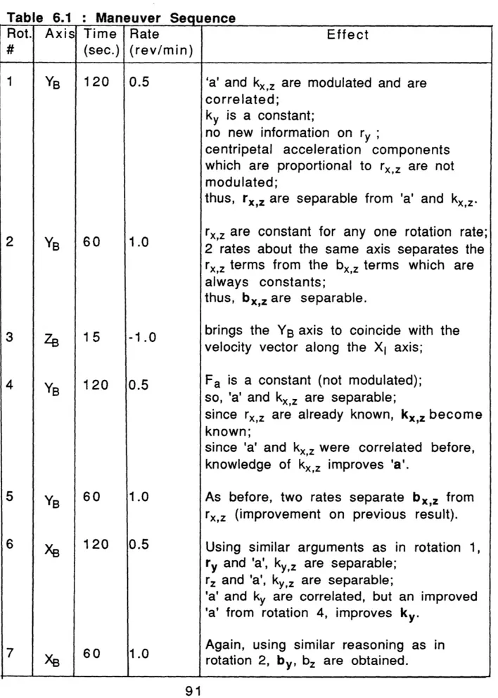
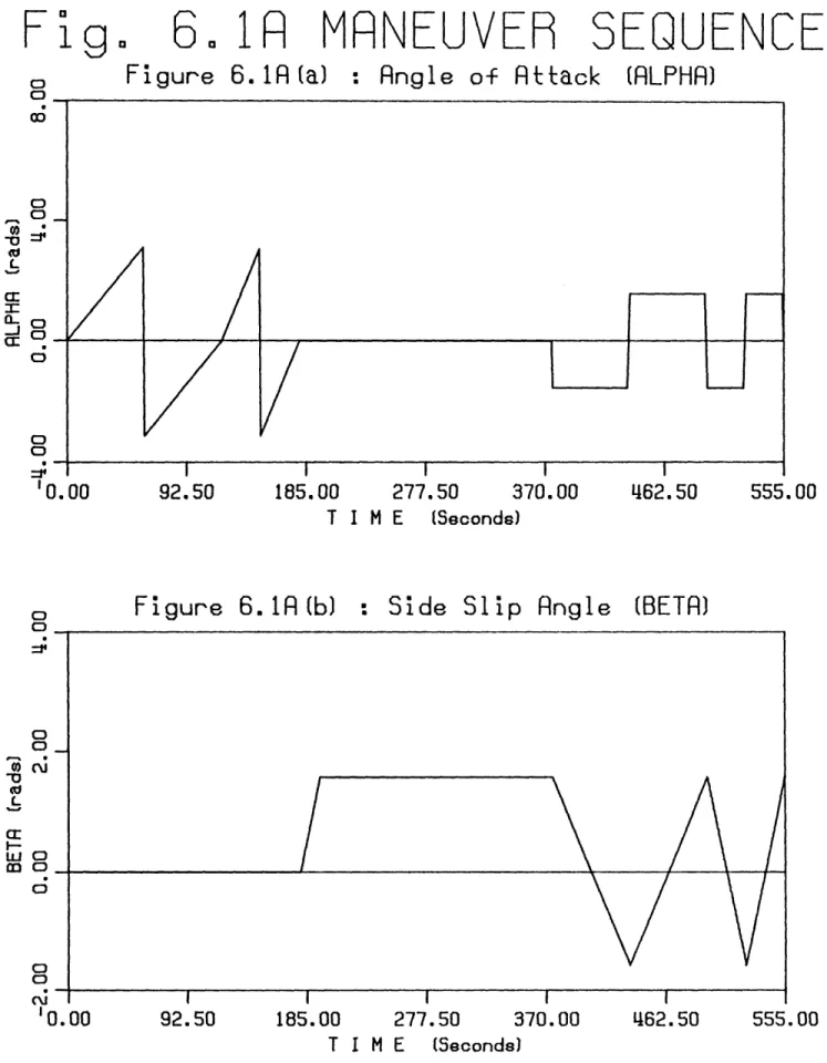
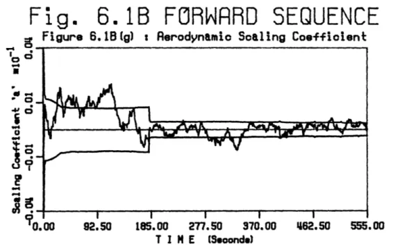
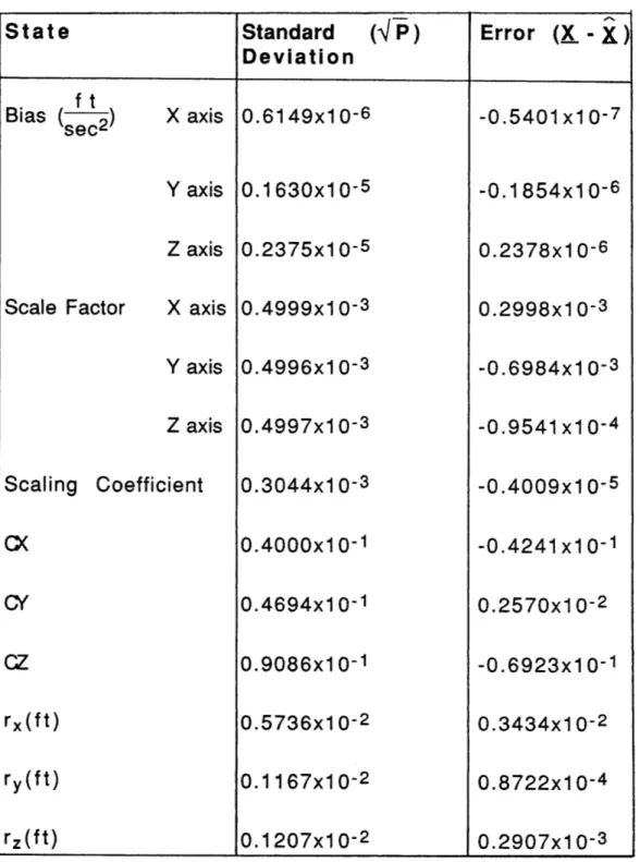
Sequence ... . 9 0 6.3 Robustness Tests... 93

6.3.1 Typical Sequence ... ... 93 6.3.2 Scale Factor Improvement ... 1 01 6.3.3 Typical Sequence in Reverse ... 109 6.3.4 Reduced R otations ... 111 6.3.5 Effects of Larger Lever Arms... 11 9 6.3.6 Effects of the Accelerometer Quantization ... 1 23 6.4 Conclusions ... 131

Bibliography

132

Appendix

Chapter 1

Introduction

1.1

Background

This thesis is part of a study conducted at Mayflower

Communications Co., Inc., for the Air Force Geophysics laboratory (AFGL) Gravity Mapping Program. The objective of the study is to determine the feasibility of estimating anomalies in the gravitational field of the earth at the Space Transportation System (STS) Orbiter

altitude to an accuracy of 1 mgal (1 micro-g) or better. On-board Global Positioning System (GPS) and Inertial Measurement Unit (IMU)

measurements will be used for this purpose. Calibration of the

accelerometers in an Experiment Inertial Measurement Unit (EIMU) is essential for its use in this project. This report documents the results of a study to estimate the errors in the outputs of these

The two phases of this experiment involve in flight, and post flight processing. In flight, the position and velocity data, the

acceleration and the orientation are derived from GPS and INS (Inertial Navigation System), and are recorded. After the flight, the INS

instruments are calibrated and aligned. Then, the above information is again derived from the two sources, with the INS data corrected for the estimated instrument errors. The information is compared, and the discrepancy is ascribed to the errors in modeling the gravity field as implemented in the INS. Thus, the difference in G is estimated.

In the accurate modeling of the Earth's gravity field, an

alternative to this space-based technique is surface measurements of the Earth's gravitational potential. This method requires

measurements as close to the generating mass as possible. However, a variety of reasons (geographic, political etc.) do not allow for accuracy and homogeneous resolution over certain land and ocean areas. Thus, the space-based technique was chosen for this study.

The low-earth orbiting vehicle chosen for this project is the space shuttle. The Gravity Anomaly Experiment instrument package will be mounted in the shuttle payload bay area.

1.2 Development

There were two methods to chose from for the shuttle-based experiment accelerometer calibration. The first technique, the Air Force Low-G Accelerometer Calibration System (LOGACS), involves the accelerometers being mounted on a precision motor turntable system. Known centripetal accelerations are generated to help estimate the bias and the scale factor errors in the accelerometer outputs. The table acts as a centrifuge with a predetermined center of rotation, and is rotated at different constant rates. Two different known rotation rates induce inputs of two different known magnitudes allowing for the separation of the accelerometer bias and scale factor errors. The table rotation modulates the component of acceleration due to the

aerodynamic effects (along the input axis), separating them from the bias errors, giving desirable results. However, this equipment is heavy (the motor table system is about 20 pounds), and thus expensive. The second calibration technique described below, gives promising results and accomplishes significant savings in size and weight.

The Fixed-Mount accelerometer bias calibration technique is a viable alternative to the Shuttle-Mounted centrifuge. Along with eliminating the need for the turntable, the Fixed-Mount technique

reduces the penalties in power, cost and reliability. It achieves these advantages with only a modest constraint on the shuttle operational procedure.

This permits a simple hard mounting of the instrument package to the shuttle payload bay area. Rotation of the shuttle at known different (moderate) rates is used to generate inputs and to modulate

aerodynamic forces. The mission specialists have to conduct rotation sequences according to the needs of the experiment. As in the first technique, the bias errors are distinguishable from the aerodynamic

effects. It will be shown that the scale factor errors depends on the knowledge of the lever arm from the CG of the shuttle to the location of the accelerometers in the experiment package. Thus, the scale factor can only be calibrated to the degree to which the shuttle center

of gravity (CG) is known.

The scale factor errors are heavily correlated with the

aerodynamic effects. The aerodynamic coefficients have a great deal of uncertainty due to the limited knowledge of the atmospheric density at orbital altitudes. Since the scale factor errors follow the

aerodynamic forces, while the lever arm errors do not (even though the uncertainty obviously causes problems in the estimation of errors), it was believed that the presence of a small aerodynamic acceleration might help to separate these errors from each other. In any case, it is shown below that the scale factor error is not crucial to the STS-GPS Tracking for Anomalous Gravitation Estimation (STAGE) mission.

As figure 1.1 (reproduced from [ref. UPV89]) shows, at the nominal shuttle altitude of 300km, the drag acceleration ranges

Drag

acceleration,

ng

101

/--

Atmospheric

Solar

max-

-

a=90

!HiRAP

i

IA

A:

aenstry variaon

(U.S. std

1966)

nin

shuttle

circular

orbit

)km)

7.1

K

AR

_E

0-1

1

=

10-5 10-4 10-3 10-2 10-1

Arealmass,

m

_/kg

100101l

1

4ACIP

105

between 0.01 to 1 gg. Accelerations due to crew activities (exceeding

1gg over short intervals) and accelerations due to vernier thruster

activity (up to about 200gg over shorter intervals) may be larger than the drag. Of these, the mission specialists can minimize their's and the vernier thruster activity. But, the aerodynamic drag persists even

while data is being taken, and must be accounted for to the desired accuracy. The 0.5% accuracy (based on ground calibration) of the MESA accelerometer selected for this mission will at maximum produce an error of 0.005gg in the presence of drag. This is an acceptable error

relative to the other elements in the error budget.

1.3 Approach

The recursive estimator chosen to accomplish the task of experiment accelerometer calibration is the KALMAN Filter. This is chosen because the filter allows data to be used from random

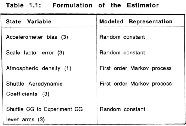
maneuvers and requires no conditions on the shuttle motion for the data to be processible. Its formulation allows for covariance analysis and the simulation to be done simultaneously. Table 1.1 below shows how the errors were modeled in the formulation of the estimator.

Table 1.1:

Formulation

of the Estimator

State Variable Modeled Representation

Accelerometer bias (3) Random constant

Scale factor error (3) Random constant

Atmospheric density (1) First order Markov process

Shuttle Aerodynamic First order Markov process Coefficients (3)

Shuttle CG to Experiment CG Random constant lever arms (3)

Chapter

2

Deriving the Measurement Model

2.1 Presentation of the equipment used

2.1.1 Experiment IMU Specifications

As discussed before, the experiment instrument package, unlike the turntable package (figure 2.1 [ref. Kar89]), is hard mounted in the

shuttle cargo bay area (figure 2.2 [ref. Kar89]). Based on the on orbit shuttle dynamics environment and the error budget of below 1lg for the acceleration measurement, the specifications set for the

experiment IMU are [ref. Upa89, page 3-9]:

Accelerometer Bias a = 10 g with 1 pg stability

(3.22x10 -_{4 ft/sec}2₎

Accelerometer Scale Factor a = 500ppm

IMU With Precision Accelerometer*

)le System

Figure 2.1 : Preliminary Packaging Concept for the

Experimental IMU (STS-GPS Tracking

Experiment)

GRAVITY ANOMALY ESTIMATION USING GPS MEASUREMENTS ONBOARD THE STS

ORBITER EXPERIMENT INSTALLATION EIMU ANTENNA -CABLE (fXISTING) UPR GPS ANTENNA (EXISTING) L-IO -VOL 7aZ< EX PE RIIIKE NT HARNESS

ANTENNA (E XIS TING)

(EXISTING)

Rockwell International

* Orbiter CG

X0 = 1093in, Y0 = Oin, ZO = 372in

* EIMU CG

X0 = 1213in, YO = Oin, ZO = 360in * Orbiter IMU CG

.i ··

Experiment IMU Availability

The industry data collected by R.G. Brown Associates, Inc. under a subcontract from Mayflower Communications Co., Inc. indicated that a strapped down IMU configuration should be used. Ring laser gyros and precision accelerometers make up the IMU instruments for this

configuration. The Honeywell advanced ring laser gyro RLG 1342 and the Bell Aerospace Miniature Electrostatic Accelerometer (MESA) were selected as the candidate instruments. The performance of this

accelerometer is given below [ref. Upa89, page 3-11]:

Manufacturer : Bell MESA 3-axis unit

Full Scale : 1 10 milli g

2 1 milli g 3 100 gg

* range (1,2 or 3) selected by the user

Resolution 108

Space Qual. yes

Size 5x9x4 (Inches)

Power 9 Watts

Weight : 5 Ibs.

Cost $500K

The advantages of using a Bell MESA accelerometer over others includes its proven technology and higher level of performance. The 2.1.2

In addition to these IMU instruments, a modified Motorola TOPEX GPSDR receiver and a Data Tape MARS 1428 Tape Recorder are also part of the experiment package.

2.2 Derivation of the instrument output

2.2.1 Equations of motion

The derivations in this chapter follow closely, unpublished notes by Professor Wallace E. Vander Velde. The acceleration sensed by the experiment instrument in the shuttle can be derived from the equations of motion. Errors in this vector can be inferred from observations of both translational and rotational positions and velocities of the

shuttle, applied to a proper model. The equations of motion for

translation and rotation are decoupled by writing them for translating the center of mass (CM) of the shuttle and rotating about that point.

a

Applied force (E) = ( Linear momentum of CM) (2.1)

E = -cm) (2.2)

E = m.4cm (23)

Here, the time derivatives are as observed from an inertial coordinate frame.

During the maneuver period the mission specialists will remain motionless and use a minimal amount of fuel to accomplish the

sequence. Thus, the mass of the shuttle can be modelled to be a constant over the interval of accelerometer calibration.

at, (l.WIlB)

Transfering to body coordinates,

M = ( I.WIB ) + WIB X (I.WIB) (2.5)

As seen from the body coordinates, I (above) can be considered a constant. Thus,

M = 1LB + WIB X (I.WlB) (2.6)

where A-lB is simply the rate of change of the shuttle's angular velocity, as seen in body coordinates.

To maintain generality, the reference body coordinate frame should be treated as not being aligned with the principal axes of the shuttle. Here, the I would be a full matrix, and a rigorous integration would be required to solve for WIB(t). Given M, integrating the

differential equation

at

gives WIB(t).

The alternative to modelling the external moment history and integrating the differential equation is specifying WIB(t) as a

sequence of rotations. This is an adequate description of the motion environment for the purpose of analyzing the accuracy of the

accelerometer calibration procedure. A sequence of angular rates can

be specified because data will not be processed during intervals of thruster activity.

2.2.2 Lever arm

As stated in Chapter 1, the experiment package will be located in the payload bay area of the shuttle. This location does not coincide with the center of mass of the shuttle. Thus, the accelerometers will indicate the accleration at a point other than the center of mass of the shuttle. To translate this information to the CM, call the position vector from the origin of the inertial frame to the location of the accelerometer La and the separation of La from Lcm (the vector from the origin of the inertial frame to the shuttle CM), L.

La = Lcm + L (2.8)

2.2.3 Acceleration vector

Here, the acceleration vector is derived. Differentiating equation

2.8,

(La)

t

a

a

"a (Lcm) + atB

()

Since the position of the accelerometers is constant in body

orbiter does not change significantly (also in body coordinates) during the period of calibration, equation 2.9 can be written as,

_t

([a) = t (Lcm) + W lB X . (2.10)

Now, differentiating again,

t2 ( a= t2

1 (Lm) + (B XL) + WIBX(WIB X ). (2.11) 1

= F + IWIBX r + WIBX L+ WIBX(WIBX r) m

As stated above assuming that L is negligible,

a2

1

(rLa) = F + IBX r + WIBX(WIB X r). (2.12)

ot 2_{1 _}

Equation 2.12 represents the acceleration vector as seen at the location of the experiment IMU. Each accelerometer indicates the non-gravitational component of this vector along its input axis. The

gravitational contribution to the specific force is balanced evenly over the acclerometer parts (as in a simple vertical spring mass system on a table) and does not create a force difference that can be indicated. Thus, comparisons with other methods that indicate the gravitational contribution allow an accurate deducement of this effect. The only non-gravitational contribution to the specific force which is of consequence here, is that due to aerodynamic effects. So, E can be written specifically as

Fa.

Non-gravitational 1F a + -IBX _{L + WIBX(WIB X r) (2.13)} acceleration

2.2.4 Accelerometer output vector

The actual indicated quantity of the accelerometers would include the afore mentioned non-gravitational acceleration and

additional error terms that need to be modelled. Only the bias and the scale factor errors need to be accounted for, because the other errors in the system are trivially small (for instance the disturbances due to outgassing, astronaut movement and vernier thrusts etc. can be

minimized at the time of the calibration). To model the set of

accelerometer outputs at any given time, define unit vectors along the input axes of the accelerometers coordinatized in body coordinates. These unit vectors (call these 1TIAi for i = 1,2,3) can be utilized to represent misalignments between the accelerometer axes and the

shuttle body axes. After adding the wideband noises (ni) to the system, the output vector is,

1+k1 0 0 0 1+k₂ 0

0

0

1+k

where ki (i=1,2,3) are the scale factor errors and bi are the biases. All the vectors in the above expression are in body coordinates.

mi

m2=

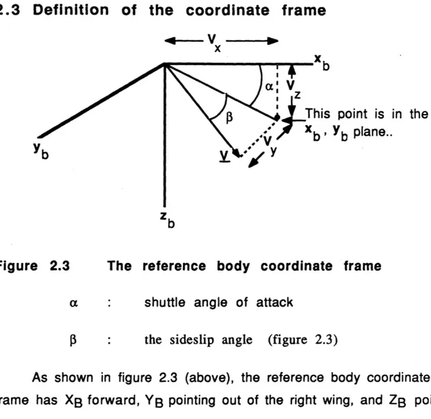
2.3 Definition of the coordinate frame

4

x

point is in the

Yb plane..

Figure 2.3

The reference body coordinate frame

a : shuttle angle of attack

S : the sideslip angle (figure 2.3)

As shown in figure 2.3 (above), the reference body coordinate frame has XB forward, YB pointing out of the right wing, and ZB pointing downward. It is assumed that the orientation of the body frame

relative to the inertial coordinates, and the velocity vector in inertial coordinates are known inputs to the filter. Thus, using quaternion

manipulations [ref. Ve183], the velocity can be transformed from inertial to body coordinates.

v(B) ₌ CIB. _(l)

Here, the transformation matrix is [ref. Ve183],

(2.14)

B I

1-2[s(2)2 + s(3)2] 2[s(1).s(3) - s(O).s(2)]

2[s(1).s(2) - s(O).s(3)] 1-2[s(1)2 + s(3)2] 2[s(2).s(3) + s(O).s(1)]

2[s(1).s(3) + s(O).s(2)] 2[s(2).s(3) + s(O).s(1)] 1-2[s(1)2 + s(2)2]

where the 's' represents the cosine (s(O)) and the sine (s(1),s(2) and s(3)) terms in Qibsind, the indicated quaternion between the intertial and the body coordinates. Now, a and 3 can be defined using Vx, Vy and

Vz, the body axis componenets of the velocity vector, and IVI, its

magnitude (figure 2.3). Using the positive directions for a and f defined in the figure,

a = tan (Vý) (-,)* (2.15)

A four quadrant arctan routine is used

V

x

)

= Sin-1 ₍

₍₂

IV'

2.4 Derivation of the aerodynamic force

The modelling of the aerodynamic force Ea poses the largest question in the formulation of this problem. A nominal model of this force and a representation of the uncertainties in that model are required for error analysis purposes. The aerodynamic force is of the form,

1

Ea = _(p)V 2_{A. f(a,J) (2.17)}

where, a, : are as defined in section 2.3

p is the atmospheric density at the orbiter altitude

V is the shuttle translational velocity in inertial

coordinates

A is the planform area of the orbiter as seen

from the z-axis (figure 2.2)

f(a,P) : the aerodynamic force coefficients, (such as

the axial and normal force coefficients).

Modelling the axial, normal and side force coefficients rather than drag, lift and sideslip coefficients, gives the aerodynamic force (Ea) directly in body coordinates (simplifying the calculations).

Dividing equation 2.17 by the shuttle mass, the scalar components that multiply f((a,) can be collected together as a coefficient 'a,' in the form of an accleration.

1 1

ma 2m (p) V2_{A . f(a,)} (2.18)

= a . f(a,( ) (2.19)

The uncertainty in 'a' is primarily due to the uncertainty in the

atmospheric density, p (which is highly uncertain at orbiter altitudes).

2.4.1 The aerodynamic force coefficients

The elements of f(a,3) are defined by the hypersonic aerodynamic characteristics of the shuttle. The components of tf(c,p) along the X,Y

and Z body axes are called Cx(a,p), Cy(ca,f) and Cz((a,) respectively. These coefficients (along with 'a' discussed before) define the axial, side and normal aerodynamic specific force in body coordinates.

For the purposes of error analysis, it is important that the

uncertainties in these effects be represented fairly. The nominal form of these functions should produce the dominant character of the

aerodynamic effects. It is not crucial that this nominal form be

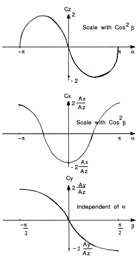
correct, since it is the error that is being estimated (a more accurate nominal form does not affect the estimate of the error). The general shape of these functions is as shown below in figure 2.4.

A = Planform area

Cz

Scale with Cos2

Cx Ax Az

2

Scale ith Cos p

It ta Ax - 2-Az Cy AZ

Figure 2.4 : Aerodynamic Force Coefficients

29 A -I2 2 i i ,,, • ' V

24

lxl'ý

The planform area of the vehicle is used as the reference area to define the force coefficients. As stated before, this is the projected area as viewed along the ZB axis (since it is the largest). Thus, when a

= +/-90deg and 3 = Odeg, the velocity vector points along the ZB axis and Oz reaches its maximum of 2. Cz is scaled with Cos2 _{P because the} component of velocity in the X,Z plane, which rotates with a, is

proportional to Cos

P,

The maximum values of ax and Cy must be scaled by the ratio of the maximum projected areas along these axes (Ax and Ay) to the

reference area (Az). Thus, the following functions define the

components of f((a,P), and represent the nominal aerodynamic specific force. Ax Cx = -2. z .Cos a Cos2 (2.20) A Cy = -2 Sinp (2.21) = Cos2 _(2.22)Az Cz = -2 Sin a Cos2 3 (2.22)

Chapter

3

Modelling the Error Dynamics

This chapter is derived from unpublished notes written by Prof. Wallace E. Vander Velde. The aerodynamic scaling coefficient and the aerodynamic coefficients are modeled as first order Markov processes, while the bias, scale factor and lever arm errors are

3.1 The Aerodynamic Force

The uncertainty in the knowledge of the aerodynamic specific force can be modeled in several ways. Yet, errors in the

representation of 'a', Cx, Cy and Cz cannot be avoided.

3.1.1 The scaling coefficient 'a'

The uncertainty in 'a' arises primarily due to the uncertainty in the knowledge of the atmospheric density, p. So, the scaling

coefficient can be expressed as,

a = an + Sa (3.1)

where, an: is the nominal value

and 8a : is the error in the knowledge of that value.

The Sa term is modeled as a Markov process, a correlated process in time. Since the atmospheric density at one point is

correlated to the value at another point by only the distance between them, 'a' has a correlation time given by,

Ia (3.2)

a V

where, I : is the correlation length of the density variations

and V: is the shuttle velocity.

1 + ts

(3.3)

1 + -rs

S a +r SSa = rn

S a + r•a= rn

Thus, the linearized dynamics of the error in the scaling coefficient

are expressed as (calling n = na, and r = ra),

1

8a = Sa + na. (3.4)

"a

Over a period of AT, AT

8a(AT) = D Sa(0 ) + f4(AT,-r).n(r).dt

The variance Va = Ga2 _{(AT) = 8a(AT)}2

= 65a(0). Sa(O)T DT + ... (other terms),

if the error is a matrix. But, since it is a scalar here,

AT AT

= D2.8a 2_{(0) + fdcn}

1 fdr2-4"(AT,r). 1 n(1r).n(r2) DT(AT,r 2).

0 0

Now, since na(t) is a white noise, the expected value is

na(t) = 0.

(3.5)

(3.6)

(3.7)

and n(r 1 ).n(r 2) = Na. 8('2 - ' 1). (3.9)

Here, Na is the intensity of the noise, chosen to give the desired standard deviation for 5a in the steady state. So, the variance becomes,

AT

= [.Sa(0)] 2 + fJ(AT,t). Na. DT(AT,r).dr. (3.10)

0 AT

where D= e', . If V, is the variance of 6a,

1 1

Va = _{(--).Va + Va. (-)+ Na. (3.11)}

ra

Ta

and since Va = 0 in the steady state,

2 Va = Na (3.12) Ta Va = T _.Na 2 Na = .Va 2 2 (3.13) Na ,a a

3.1.2 The aerodynamic coefficients

The aerodynamic force depends on a (the angle of attack) and P (the sideslip angle). Therefore, to represent the uncertainty in f(a,3), the general dependence of the aerodynamic forces on a and

f

the coefficients Cx, Cy and Cz, and adding the error terms to the nominal components, they can be expressed as,

Ax

Cx = -(2 5+ _{Cx). Cos a Cos}2 _{3 (3.14)}

Cy = -(2 y+ &Cy).Sin P (3.15)

Cz = -(2 + 8_{Cz). Sin a Cos}2 _{3 (3.16)}

Clearly, the error terms (8Ci, i=x,y,z) in equations 3.14, 3.15 and 3.16 are correlated processes. If their dependence on a and 3 were correct and only the magnitude scaling were wrong, these errors would be random constants. But, since the modeling of the dependence on a and P is in error to some extent as well, 8Ci should be modeled as being variable with a correlation time that depends on how rapidly a and P change. So, as in the case of the scaling

coefficient, the dynamics of 8Ci are (for i=x,y,z),

sci = .8Ci + nci. _(3.17)

with Tc = 3w'

1 3

or, rearranging, 1c = .w (3.18)

where, _{w = The shuttle angular rate =}

Iwibl-Following a similar procedure as before, the intensity of the white noise process nci(t) is,

Nci - . ci Plugging in for Trc,

Nci = . w. C (3.19)

This completes the modeling of the uncertainty in the representation

1

of

_m-

3.2 The rotation rate

The errors in the knowledge of Wib and Wb are two other errors in the representation of the specific force at the accelerometer location. Data on W-ib and Wib will be derived from the ring laser gyros of the experiment IMU which are of type Honeywell GG1342 [ref. Kar89]. Therefore, the principal short-term error source is the quantization error. Wib is evaluated as,

1b(tk)

= •e- i (3.20)

where the sum is over the Ae pulses accumulated during the current sample period. This gives,

Wib(tk) = AT (W1 b(tk) - Wib(tk-1) )' _(3.21)

or a higher ordered differencing rule can be used for a more accurate value. In any case, the quantization error effect is correlated in W.ib

and Wib, and these terms enter the specific force expression nonlinearly as well. So, an exact treatment of this small gyro quantization error is difficult.

As a solution to this problem, the variance of the wideband noises nl,n2,n3 are augmented with terms representing the

magnitude of the quantization error effects in Wib and Wib. The perturbed W components are discussed in section 4.3.

The mission situation envisioned has the shuttle doing a sequence of rotations about different axes. Since these are controlled maneuvers, the rotations are modeled as each having constant angular velocities. Thus, during the times that

measurements are processed, Wib = 0. In an actual implementation, the Wib x r term should be included because the angular velocity may not be exactly constant. But for the simulation of this mission, this term is omitted because the perturbations in the angular velocity are assumed negligible.

3.3 The lever arm

The error in the knowledge of the lever arms (r) is important as it is largely inseparable from the accelerometer scale factor errors. As shown in the output vector in Chapter 2, the r multiplies the scale factor contribution (ki) to the output. The atmospheric

1

force is actually helpful in this regard as IEa modulates the effect

of the ki on the measurements, while not influencing the effect of .r on them. So, in theory, these errors become less heavily correlated when the aerodynamic forces are modulated along the axes of the centripetal acceleration components, which are proportional to the lever arm components. This can be accomplished by rotating the shuttle about an axis that is perpendicular to the lever arm.

The knowledge of r is in error primarily because the

accelerometer location is referred to the shuttle center of mass. Thus, r is known only as well as the CM location of the shuttle is, and it is not known to the required accuracy. By supposing that the center of mass location is essentially fixed during the calibration period, Lr is modeled as a random constant.

3.4 The dynamics of the

state

The state vector to be estimated is,

a

(3.22)

IE

L

The four vectors b, k, R and [r, and the scalar 5a, give a total of 13

state variables.

The dynamics of this state are of the form,

X= AX +n. (3.23)

As discussed before, the scaling coefficient and the

aerodynamic elements are modeled as Markov processes and have diagonal elements in the A matrix. 'A' has values of zero

corresponding to all the other states since they are all modeled as random constants. The noise vector,

nT[= 0 0 0 0 0 nn a ncx ny ncz 0 0 0] (3.24)

is also made up of zeros for the rest of these states. In equation form, the dynamics are,

1

X7 _ra X7 + na (3.25)

(3.26)

(3.27)

(3.28)

Chapter

4

The

Kalman Filter

4.1 Introduction

The introduction to KALMAN filtering is a section from [ref. Kar89, pages 42-45]. It is reproduced here for the completeness of this document.

The dynamics of the accelerometer calibration process which describe the system, have been presented in earlier chapters. Using this information, a recursive KALMAN filter is designed. This design involves various tasks; discretization, measurement processing, covariance analysis and propagation - that are now studied. This complete model of the filter is later implemented on a digital computer.

Techniques used in the filter design are fairly general and can be transposed with minimal adaptations to other applications. The same structure was used in the Attitude Alignment Transfer

problem [ref. Kar89].

4.2

Introduction to KALMAN Filtering

This section is taken from [ref. Kar89]. It summarizes important results about KALMAN Filtering techniques. A more

detailed presentation can be found in the engineering literature, e.g [ref. Cor88, pages 102-155] and [ref. Bro83, pages 181-212].

Optimal filtering of a linear system refers to estimating the current state, based upon all past measurements. Starting with a dynamic system and a corresponding measurement relationship:

Xk+1 = ýkXk + Vk (4.1)

Zk = HkXk + wk (4.2)

where:

Xk = (n x 1) state vector at time tk.

k = (n x n) state transition matrix.

wk = measurement noise - white sequence with assumed known

covariance (uncorrelated with the vk sequence).

Zk = (m x 1) measurement vector at time tk.

Hk = (m x n) observation matrix.

vk = (n x 1) driving noise vector - white sequence with known

covariance.

if i = k (4.3) {Q Rk if k

E[wkwTi] =

if

_k

_(4.4)

E[wkvTi] = 0 for all k and i (4.5)

Denoting the estimate prior to the incorporation of the latest measurement with a 'minus' superscript, the estimation error is defined as:

ek- = Xk - Xk - (4.6)

and a third covariance matrix is introduced, the state error covariance matrix:

Pk- = E[ek-ek-_{T] (4.7)}

An update of the estimate is obtainable through blending of the prior estimate and the latest measurement. In general:

Xk = Xk- + Kk(Zk - HkXk-), (4.8)

(In _{this analysis, Xk = Xk- + Kk(Zk(X) - Zk(~)} ).

where Kk is a blending factor matrix determined in such a fashion that the optimality criterion is satisfied. Through algebraic manipulation, Kk is found to be:

Kk = Pk-.HkT(HkPk-HkT + Rk)- 1 _(4.9)

and this value is called Kalman gain. The state error covariance for the updated estimate is:

Pk = (I - KkHk)Pk- (4.10)

Between measurements, the filter propagates both the estimate and

the error covariance in accordance with the equations:

Xk+ 1 = _kXk (4.11)

(4.12)

Pk+1-1 = OkPk kT+ OQk

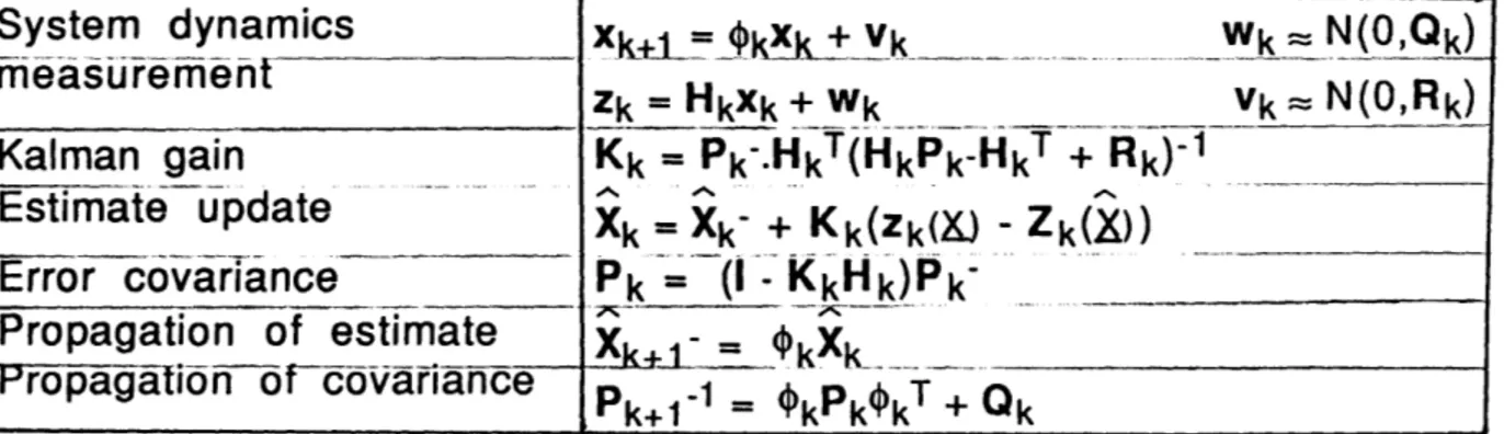
Table 4.1, given below, summarizes the equations evoked in this section. A detailed expression is now sought for each of the terms mentioned.

Table 4.1 : The KALMAN Filter loop

System dynamics xk+_l _ Vk Wk _N(0,Qk) zk = HkXk + Wk _{Vk= N(0,Rk)} Kalman gain _{Kk = Pk-.HkT(HkPk-HkT +} Rk)-1 Estimate update _{Xk = Xk- + Kk(Zk(.) - Zk(X))} Error covariance Pk' -( KkHk)Pk Propagation of estimate Xk.= kX Propagation o-fcovariance Pk+- = kPkk T Qk

4.3 Discretization of the dynamics

To implement the filter on a digital computer, in a case where measurements are processed only at discrete points in time, the dynamics need to be discretized. As shown in section 4.2, these dynamics in discrete time are,

X(tk+l) = 4D.X(tk) + V(tk). (4.13)

where, (D and V(tk) are as shown below.

0 0 0 0 0 0 0 0 0 0 0 0 0 0 0 0

0

0

0

0

0]

_(4.15)

2 (e-2AT

•v7 = (1 e-2 _a)

a2i =2i (1 e-2A T

=

C

r

)

In equation 4.17, the 22i 's , Oy and o2z respectively.

i=8,9,1 0

(4.16)

4.4 Measurement

processing

The measurement equation combines all the elements

discussed so far and simulates the measurement. The form of the ith measurement is,

T

Mi = (1+ki). 1Ai.S + bi + ni . (4.18)

T

As before, 1TAi (for i=1,2,3) defines transposes of unit vectors along the input axes of the accelerometers coordinatized in body

coordinates. The bias terms (bi) and the scale factor terms (ki) remain as shown before. The components of the noise term (ni)

include the wideband accelerometer noise (see 'R' matrix derivation) and an estimate of the effect of the quantization error in the Wi components. The S vector represents a model of the aerodynamic

1

specific force (•-F), the centripetal acceleration ( WVx(W.xr) ), and

the tangential acceleration due to the angular acceleration (Wxr), making the assumptions mentioned in Chapters 2 and 3.

-8Cx.Cosa.Cos 2_P

S = (a + Sa) P + -8Cy.SinI3 + WMX.r (4.19)

-L Cz.Sina.Cos 2p

Here, P is defined using nominal quantities for the aerodynamic specific force (as in equations 2.20, 2.21 and 2.22).

Ax -2. AzCosa.Cos2p Ay -2. -Sinp -2.Sin -2.Sina.Cos 2 -(4.20) p =

WMX refers to a matrix made up of three vectors Wx, Wy and Wz. WMX =

[A

Wx

-(wy2+Wz2)Y

W

]

w

wxwz

and Wx,Wy and Wz are nominal values of the rotation rates about the

respective body axes. Finally, the L vector consists of simply the components of the lever arms and their error terms,

rx + •rx

L = ry + 8ry (4.25)

rz +

Srz-The measurement perturbation from nominal is (from 4.2),

5M = H.•, + D (4.26)

where the H matrix (defined using equations 4.18-4.25) is given in the next section.

The BS vector is defined differently depending on whether it is used to derive the system's observation matrix, H (for the 'real'

phase), or the measurement vector, Z (for the simulation). In the

error estimation step, when deriving the H matrix (using X values), the noise due to the gyro quantization effects are added to the rotation rates.

Wi = Wi + Wi (4.27)

where BW i is a uniformly distributed random variable in the interval

AO AO

(-2AT 2AT). The gyro quantization value is, 1

AO =1 arcsec. = .10(rads) = 4.848x10 -6_{. (4.28)} 3600

Also, the transformation matrix for the velocities (section 2.3) is

calculated using the indicated values of the quaternions between the

inertial and the shuttle body coordinates (describing the rotation of the shuttle). These quaternions include normalized error terms defined as gaussians (AQ(i), i=1,2,3), having variances (OQG2) of the

laser gyro quantization effects.

1

oaG -= j1 .A = 1.400x10 -6. [ref. Upa89, page 5-22] (4.29)

Thus, the normalized error term is,

The quaternion between the body coordinate frame and the indicated value of the body coordinate frame (the error term) is calculated as, Qbsbsind(1) = time tag for the program (4.31)

Qbsbsind (2) = Cos 2rmali_{zed A (4.32)}

AQ(j) .Sinnormalized AQ

(4.33)

Qbsbsind (i) = normalized AQ 2

where i=3,4,5 and j=1,2,3 respectively. Now, the indicated value of the quaternion between the inertial and the body coordinates,

Qibsind, is given by multiplying its true value, Qibs (representing the rotation of the shuttle) and Qbsbsind.

When the measurement vector (Z) is processed (using X values) during the simulation phase, the afore mentioned quaternions (Qibs)

are updated with the change in the orbiter attitude, with no noise terms added. These quaternions are then used to define the

transformation matrix (section 2.3). Also, the S vector is calculated using nominal rotation rates.

The simulated measurement noise is derived from the covariance matrix for the wideband measurement noise, R (see section 4.5.3). Since R is symmetric and positive definite, a gaussian elimination can be performed on it to separate it into an LDLT (L=lower, D=diagonal) [ref. Str86] form. LDLT is further manipulated to give,

by taking the square root of D, and letting

F = LV/D.

The measurement noise, fn, is generated in the simulation as,

n = Fg,

where,

ql

. = q2 ,

_q3-and the qi are independent gaussian variables with zero mean _q3-and o=1.

Note that qqT is an identity

nnT = FgT FT = FFT as desired. 4.4.1 matrix. Thus, (4.38)

The Measurement Residual, R

The simulated measurement vector Z., and the estimated

measurement vector ZHAT are used to define the innovation vector R (Residual). R is used to update the state estimates.

(4.35)

(4.36)

As discussed above Z and ZHAT are derived according to the measurement equation (4.18), using the appropriate components. The

measurement, Z, is simulated using the true values of all the

variables, and noise is added. ZHAT is formulated using the estimated values of the variables, and no measurement noise is included. This gives the innovation vector to be,

4.5 The Observation

The observation matrix H, is derived from equations 4.18 to 4.25. The elements are presented below.

H11 H₁₂ H₁₃ = 1 = 0 = 0 H14 = 11A1T.S H15 H₁₆ H₁₇ = 0 = 0 = 1IA1T.P H18 = -a(1IA1)x.Cosa.Cos 2p H1 9 = -a(1A1)y.SinP H110 = -a(1,A1)z.Sina.Cos 2p H_{111 = 1IA1T.Wx} H112 = 1IA1T.Wy H11 3 = 11A1T.Wz H_{2 1} = 0 Matrix, (H)

H₂₂ H₂₃ H₂₄ = 1 = 0 = 0 H2 5 = 1IA 2T.s H_{2 6} = 0 H2 7 = lIA2T.P H₂₈ H₂₉ = -a(llA2)x.Cosa.Cos 2p = -a(llA2)y.SinA H2 10 = -a(11A2)z.Sina.Cos23 H2 1 1 = 11A2T.Wx H2 1 2 = 1IA2T.Wy H_{2 1 3} = 1IA₂T.Wz H_{3 1} H_{3 2} H₃₃ H₃₄ H_{3 5} = 0 = 0 = 1 = 0 = 0

H3 6 = 1IA3T.s H3 7 = 1IA3T.P H38 = -a(lIA3)x.Cosa.Cos2p H3 9 = -a(llA 3)y.Sinp H_{3 1}0 = -a(lIA3)z.Sina.Cos2p H_{3 1 1} = 11A₃T.Wx H_{3 12} = 1IA3T_.Wy H_{3 13} = 1lA3T.YWz m

4.6 Covariance Analysis

4.6.1 Introduction

This section deals with the covariance matrices used in the KALMAN Filter. As stated before, the covariance analysis is performed simultaneously with a systematic simulation. This enhances the results because studies have shown that doing a covariance analysis exclusively would not be as conclusive [ref. Cor88, pages 277-280].

4.6.2 The Driving noise, Q Matrix

This matrix is a part of the covariance matrix propagation relation. Since all the states are modeled as random constants except for the aerodynamic scaling coefficient 'a,' and the force coefficients CX, CY and CZ, the Q matrix is mostly filled with O's. The four states mentioned above are Markov processes, which take the simple form shown below.

o 0 0 0 0 0 0 0 0 0 0 0 0

o

0 0 0 0 0 0 0

0

0

0

0

0

0

o0

where a27 and v2i (i=8,9,10) 4.17.

4.6.3

are as defined in equations 4.16 and

As shown in the KALMAN Filter equations 4.10 and 4.12, the state error covariance, Pk, is updated and propagated as a function of

4kQk,Hk and Kk. Since these matrices are incremented during every time step, only the initial value of Pk, (Po) needs to be defined, the

values being obtained recursively.

0 0 0 0 0 0 0 0 0 0 0 0 2 Gb 0 0 0 0 0 0 0 0 0 0 0 ok2 0 0 0 0 0 0 0 0 0 0 0 0k2 0 0 0 0 0 0

S

S

0

0

0

0

0

0

0

0

0

0

0

0

0

0

0

0

0

0

The Measurement Noise, R Matrix

This section is derived substantially from unpublished notes written by Prof. Wallace E. Vander Velde of MIT. R is the covariance matrix for the wideband measurement noise. This noise consists of the direct wideband accelerometer error, and the effects of the wideband gyro noise propagating through the computation of the acceleration vector as seen at the location of the experiment IMU (from equation 2.12),

1

mFa + ZlBxr + WlBX(WlBxr). (4.40)

4.6.4.1 The Aerodynamic Effects

1

As discussed before, the

_m

1

a = 1 pV2.Az (4.41)

a2m

and, f(a,p) = (4.42)

Repeating equations 2.20, 2.21 and 2.22 the suggested representation of these aerodynamic coefficients is,

Ax Cx = -2 A-.COs Cos2p (4.43) A Cy = -2 A. Sin3 (4.44)

Y Vz

Cz = -2 Sino Cos2_p3

Recapping, the indicated quaternion (with noise terms) from the inertial to the body coordinates (qIB) is used to transform V(I) to V(B), and a and P are computed from the components of V(B). The indicated quaternion contains wideband noise due to the gyro quantization error. This error, independent for gyros x, y and z, propagates from LAei to qIB to CI to V(B)and then to a and P. This involves a complex, nonlinear train of calculations. But, a

reasonable approximation would be to assume a model for the computed values of a and P with independent errors of the same magnitude as the original gyro errors, instead of following the individual gyro errors through the calculations.

Under this assumption,

Ax Ax

SCx = +2 A~z.Sina.Cos 2p.a + 4 A•Cosa.Cosp.Sinp.8p

Ax

= 2 •-(Sina.Cos 2_{p3.8a + 2.Cosa.Cosp.Sin3.8p) (4.46)}

Ay

8Cy = -2 A Cosp.sp (4.47)

T--Z

8Cz = -2.Cosa.Cos2fp.5a + 4.Sina.Cosp.Sin3.8p

= 2(-Cosa.Cos2 _{3.8a + 2.Sina.Cosp.Sinp.8p), (4.48)}

where 8• and o3 are independent gaussians with ao = = 2

Si = OGQ. Thus, the individual terms of 5Ci (i=x,y,z) can be squared separately and

the cross correlation terms that multiply S• and 53 disappear, 2

somewhat simplifying the computation. The OGQ is derived from the

AO as shown earlier.

The covariance matrix for the errors in indicating the vector 1

IF

MI-a

= (2a )2(Sin2a.Cos4p + 4.Cos2_a.Cos2_p.Sin2 _{). GQ2}

= (2a xz Cosp)2(Sin2a.Cos 2_{3 + 4.Cos2a.Sin2P)o 2}

CF12 = a2_{. 5CX.8CY}

= -4a2 _{.Ax A 2.Cose.Cos2p.Sin3.o2}

= -8a2 _-8a2 A AyC _{-A Coso. .Cos}s Co 2p.i _1.Sinp3.oa.2

Az I z O (4.51)

CF13 = a2. 8CX.8CZ

= 4a2.z (-SinAa.Cosa.Cos4 + 4.Sina.Cosa.Cos2 Sin2_{p) 2} (4.49)

4Sin 2_p3)~ (4.52) (4.53) (4.54) (4.55) (4.56) (4.57) )s2p) 2 2P) o(4.58)

Since 8a and 831 are not related to the original gyro quantization 1

errors, the errors in indicating the -Fa term are treated as being independent of the errors in indicating the remaining two terms. The correlation among those error contributors is tracked carefully because those two terms depend more directly on the gyro

quantization errors.

4.6.4.2 The Angular Rate

The angular rate is indicated as,

WIB = . (4.59)

where the Ae1 represent the individual pulses from the laser gyros.

1 The Ae count may be in error due to quantization by as much as ±-Ae

where Ae is the gyro quantization (referred to before). Calling the error at cycle k, w (k),

1

.6w(k) = A h T (4.60)

where _6.k is the set of gyro quantization errors at cycle k.

4.6.4.3 The Angular Acceleration

The angular acceleration is indicated as a backward difference of angular rate values.

1

The error in this quantity is, 1 I (~TW_(k) - W.(k-1)) (4.62) AT 1 S AT2 2 - k-1) (4.63)

From equation 4.41, the two terms whose combined errors that are being evaluated are,

tt = WiBxr + WIBx(W.iBxr ) . (4.64)

In this analysis, the error in knowledge of L is not a wideband error; it is a state variable. Here, only the wideband error is evaluated. So, the only interest in this context is the wideband gyro error - the quantization error - which propagates through the indicated values of WMIB and aIB.

L.t = (fLxr) + [WMx(WiBxr) + WrBx(8Wxr)] (4.65)

Now, using equations 4.61 and 4.64, =(AT2 (.qk - .q-k-1)x-) +

[1

=

[

'iQkx(WIBxLr)

+ WMIBx(

-L-LUxr

)

(4.66)

Given below are standard cross product rules,

VlxV2 = -Y 2xV1 (4.67)

Using equation 4.68 and 4.69,

= (- L X (ak - -k-1 ) - (W.IBxt) x _(qk + _{AT (WIB.-).•qk}

1

I( WIB·hgk)' _(4.69)

where the first and second terms are derived from equation 4.67, whereas the third and fourth terms are derived from equation 4.68.

6tt

=

(-T2

L

x

Dak

+

L XI-)

(AIBxr) x

k

(AT - 7Tr).bk r.WTI

1 _A• ' W TIB _.a - ' ) _- 1_{-AT -L-WTIB--k} (4.70) Now, combining the .qk and _.k-1 terms,

S-

+

(W

x

Qk

+

(-r

x

1 ₁

_

' (Mv T IB '_L)'•- k

--T WTIB'-k _(4.71)

Defining the term within the square brackets as U,

1 ₁

.t

=

-[u

x]

g

+T2[L

_x

_{k-1 +}

_k-TIBVr)'l'k

0 _{-Uz Uy}

[Ux]

U

0

-U

(4.74

-Uy Ux 0

Separating the 5gk and _.k-1 terms and simplifying the htt equation,

itt = Mk-b-k + Mk-l.-.bk-1 (4.75

where,

1 1

Mk = -[U x] + (WTIB.L).I - ¥T r.WTIB (4.76

1

Mk-1 = T2 [1 X] (4.77

The quantization errors are zero mean, and -qk is treated as being independent of .k-1. Thus, the covariance matrix for the wideband errors in the two terms is,

8tt..ttT = Mk-. -k.-T .MkT + Mk-1.- qk-1 . k-1T .Mk-1T (4.

The quantization errors of the different gyros are independent of each other. S .,. 2

Wk--WkT

=

oGQI

where oGQ is the variance of the gyro quantization error, calculated

as shown before (equation 4.29),

2 1 OGQ = 1 2 (AO)2. (4.81

)

I)

)

1

The quantization error is uniformly distributed over -A• , where

Ae is the pulse value of the gyro output.

= [MkMkT _{+ Mk-1-Mk-1}T_{] .a}

Q (4.82)

Now, the covariance matrix for the wideband noise in the computed vector,

1

W = mFa + ABxr + WIBX(WIBXT). (4.83)

is,

-.6WT = CF + 4tt._T . (4.84)

The form of the measurement without the scale factor and bias errors, which are not wideband, is

M = AW + n (4.85)

where,

T

A

= 1

J

(4.86)

and n is the vector of wideband accelerometer errors - which is primarily the quantization error. n is independent of the error in indicating W. So, the covariance matrix for the wideband

measurement noise is,

= A. .WT .AT + l.nT

= A.

jW.WY.

with, 2 1 0

_{AQ =}

_yj(AV)

f

(4.88)

S

Chapter 5

Software

Presentation

5.1 Introduction

This chapter contains a description of the software designed to evaluate the accuracy of the calibration of an experiment

accelerometer package on board the shuttle. Significant portions of this chapter are taken from [ref. Kar89] since the structure of the

program is fundamentally the same. This package allows for various simulation schemes to be tested and can be used to validate the model. With minor adjustments, it can later be used to process actual flight data.

The program is written in Fortran [ref. RP83] and contains 36 subroutines and 8 functions piloted by a main program called EXEC.

In addition 2 data blocks and 6 common blocks gather all the numerical values and variables relevant to the system.

The software follows the pattern described in the modeling of the dynamics and the KALMAN Filter formulation of the calibration problem. It not only outputs covariance results, but also computes a sample history of state estimates. Another property mentioned

before is its ability to process measurements regardless of the trajectory of the shuttle. So rotations and maneuvers not related to the experiment may also produce useful data. The following

sections, substantially derived from [ref. Kar89] (as mentioned above), present a flow chart of the program and a brief description

of its relevant characteristics. The code itself (in Fortran), is given in Appendix A.

Note : With additions (of existing subroutines) to the program, a UDUT of the output matrices can be performed for clarity. Also, the program structure (with minimal modifications to existing

subroutines) allows for real data to be read in and processed.

5.2 Looping

The organization of the ALTRANSS [ref. Kar89] software is preserved. It is organized in three basic levels - nested in one another.

The first level is the level of the loop 9000 and

represents a 'run'. A run can be performed with a fixed or different randomization of the variables. Only the

Monte-Carlo processing module (which is not used for this application) is outside this loop.

The second level in depth is the level of the loop 900 and represents a 'measurement processing'. It is executed every time a measurement reaches the sensor during the maneuver phase. Modules controlling the maneuver

parameters and initialization of the filter are outside this loop.

The third and last level is the level of the loop 20 and represents a 'time step'. It is executed at a frequency

chosen by the user - normally the measurement rate

-and performs the real-time propagation of the state, the state estimate and the covariance. Modules controlling the output of results and measurements lie outside this loop.

Loop 20 is executed a finite number of times per loop 900 run, which in turn is performed a finite number of times per loop 9000

run. For simulation oriented results, the loop 9000 is only run once. The looping and nesting aspects are shown later in the flow chart.