Advances in the visualization and analysis of boundary layer flow in swimming fish

(1)

ADVANCES IN THE VISUALIZATION AND ANALYSIS OF BOUNDARY LAYER FLOW IN SWIMMING FISH

By Erik J. Anderson

M.S., Saint Francis Xavier University, 1998 B.S., Gordon College, 1989

Submitted in partial fulfillment of the requirements for the degree of Doctor of Philosophy

at the

MASSACHUSETTS INSTITUTE OF TECHNOLOGY and the

WOODS HOLE OCEANOGRAPHIC INSTITUTION

February 2005

The author hereby grants to MIT and WHOI permission to reproduce paper and electronic copies of this thesis iwhflle or ioart ,ld to distribute them publicly.

Signature

of

Author

_

_-Joint Program in Oceanograph /Applied OceSience and Engineering Massachusetts Institute of Technology and Woods Hole Oceanographic Institution

/ February 2005 Certified by Certified by Certified by 4 -, % 0/ -- -v / Mark A. Grosenbaugh Thesis Supervisor Wade R. McGillis Thesis Supervisor __ _ _ I= .1 Mark A. Grosenbaugh

Chairman, Joint Committee for Applied Ocean Science and Engineering

MASSACHUSETS INST E? Woods Hole Oceanographic Institution

(2)

(3)

Advances in the visualization and analysis of boundary layer flow in swimming fish By

Erik J. Anderson

Abstract

In biology, the importance of fluid drag, diffusion, and heat transfer both internally and externally, suggest the boundary layer as an important subject of investigation, however, the complexities of biological systems present significant and unique challenges to

analysis by experimental fluid dynamics. In this investigation, a system for automatically profiling the boundary layer over free-swimming, deforming bodies was developed and the boundary layer over rigid and live mackerel, bluefish, scup and eel was profiled. The profiling system combined robotics, particle imaging velocimetry, a custom particle tracking code, and an automatic boundary layer analysis code. Over 100,000 image pairs of flow in the boundary layer were acquired in swimming fish alone, making spatial and temporal ensemble averaging possible.

A flat plate boundary layer was profiled and compared to known laminar and turbulent boundary layer theory. In general, profiles resembled those of Blasius for sub-critical length Reynolds numbers, Rex. Transition to a turbulent boundary layer was observed near the expected critical Rex and subsequent profiles agreed well with the law of the wall. The flat plate analysis demonstrated that the particle tracking and boundary layer analysis algorithms were highly accurate.

In rigid fish, separation of flow was clearly evident and the boundary layer transitioned to turbulent at lower Rex than in swimming fish and the flat plate. Wall shear stress, ,,

forward of separation was slightly higher than flat plate values. Friction drag in rigid and swimming fish was determined by integrating ro over the surface of the fish. The

analysis was facilitated by the definition of the relative local coefficient of friction. In general, there was no significant difference in friction drag between the rigid-body and swimming cases. In swimming, separation was, on average, delayed. Therefore, pressure drag was estimated on the basis of thickness ratio and used to calculate an upper-bound total drag on a swimming fish. Total drag was used to determine the required muscle power output during swimming and compare that with existing muscle power data. zo and boundary layer thickness oscillated with undulatory phase. The magnitude of oscillation appears to be linked to body wave amplitude.

(4)

(5)

The author is grateful for the funding received from the Office of Naval Research, Grants N00014-99- 1-1082 and N00014-96-1141, the MRI program of the National Science Foundation, Grant OCE-9724383, the National Science Foundation Graduate Research Traineeship in Coastal Oceanography, the WHOI Ocean Ventures Fund, the WHOI Academic Programs Office, and the MIT Department of Ocean Engineering.

The author thanks his thesis supervisors Mark Grosenbaugh and Wade McGillis for their guidance and enthusiasm though the entire course of this extensive experimental work. The author also thanks Mike Triantafyllou, whose feedback concerning fish

hydrodynamics played an important role in guiding the inquiry. The author thanks Larry Rome (UPenn) for his contributions as an external committee member and his critique of the work from a biological perspective. The author also thanks John Farrington, Judy McDowell, Paola Rizzoli, Ronni Schwartz, Marsha Gomes, Julia Westwater, Marcey Simon, Stacey Brudno Drange, Stephen Malley, Dominique Jeudy, and the rest of the administrative staff of the MIT/WHOI Joint Program and the Ocean Engineering student administrative staff for their dedication to the success of all the students in the Joint Program. The author thanks the faculty and staff of the MIT Department of Ocean Engineering and the WHOI Department of Applied Ocean Physics and Engineering. The author thanks John Trowbridge for serving as defense chair.

Many others made invaluable contributions to this project. The author thanks Kyle McKenney (MIT, UROP) for three summers of help 'collecting specimens', meticulously cataloging thousands of images and data files, and monitoring data analysis. The author thanks Jay Sisson for engineering support and his management of the resources of the Rhinehart Coastal Research Center. The author also thanks Bruce Tripp and Bebe McCall for their administrative support at RCRC. The author thanks Rick Galat, Fred Keller, Bruce Lancaster, Joe Connolly, Mike Cifelli, and all the staff responsible for the functioning of the experimental facility. The author also thanks Ann Stone, Nancy Stedman, Keith Bradley, Houshuo Jiang, Sean McKenna, Steve Fries, Debbie Schafer, Fred Baker, Eileen Wicklund, Arden Edwards, Oscar Pizarro, Mark Rapo, Scott Gallager, Bruce Woodin, WHOI Housing and WHOI Security.

Finally, the author thanks his parents, sisters, family, friends, his wife, Rachel Anderson, and the Lord, Jesus Christ, for encouragement and strength.

(12)

ii. List of figures

1.1 Illustrative boundary layer profiles

2.1 Turbulent and laminar flat plate boundary layer scaled according to law of the wall 3.1 Set-up for flow visualization

3.2 Double exposure showing particle pairs

3.3 Fish boundary layer profiles compared to Blasius and the law of the wall 3.4 Fish boundary layer profiles compared to Falkner-Skan

3.5 Time-averaged local coefficient of friction on swimming fish 3.6 Boundary layer parameters vs. fish body position

3.7 Time-averaged local coefficient of friction for scup at x/L = 0.5

3.8 Local coefficient of friction and boundary layer thickness vs. body phase 3.9 Ue and Ve vs. body phase

3.10 Time series of normal velocity profiles on swimming fish 3.11 Boundary layer development over scup swimming in still water 3.12 Boundary layer profile time series showing incipient separation 3.13 Friction coefficients on swimming fish

4.1 Scaled sideview images of four fish species examined 4.2 Image of flume

4.3 Image of flume test section 4.4 Laser and sideview camera robot

4.5 Boundary layer and nearfield camera robot 5.1 Illustration of DPIV

5.2 Illustration of conventional DPTV

5.3 Illustration of the 'forced-monotonic' filter for near surface glare determination 5.4 Computer generated image pair used in description of particle tracking code 5.5 Plot of all potential particle tracks

5.6 Plot of track distance vs. track angle for all potential tracks 5.7 The track plot image, or matrix

5.8 Kernel multiplication for density score 5.9 Track selection process

5.10 Results of particle tracking example

5.11 Particle tracks and profiles for flow 10 cm upstream of the flat plate 5.12 Velocity field for flow 10 cm upstream of the flat plate

5.13 Particle tracks and profiles for flow at x = 21.3 cm on the flat plate 5.14 Velocity field for flow at x = 21.3 cm on the flat plate

5.15 Particle tracks and profiles for flow at x = 32.3 cm on a swimming bluefish 5.16 Velocity field for flow at x = 32.3 cm on a swimming bluefish

5.17 Comparison of conventional DPIV and PTCV

5.18 Transverse body surface motion from nearfield camera view

(13)

6.1 Flume test section profiles at 98 cm/s, blank inlet barrier 6.2 Flume test section profiles at 98 cm/s, large grid inlet barrier 6.3 Power spectra of fluctuations in mean flume profiles

6.4 u velocity field near inlet with the large grid barrier

6.5 Boundary layer profiles over flat plate, U = 33.0 cm/s, blank inlet barrier 6.6 Boundary layer profiles over flat plate, U = 68.7 cm/s, blank inlet barrier 6.7 Boundary layer profiles over flat plate, U = 117 cm/s, blank inlet barrier 6.8 Boundary layer u-profile at x = 29.4 on flat plate fit to the law of the wall 6.9 Boundary layer profiles over flat plate, U = 117 cm/s, small grid inlet barrier 6.10 Coefficient of friction vs. length Reynolds number for all flat plate experiments 6.11 Relative coefficient of friction vs. relative position for flat plate data

6.12 Relative coefficient of friction vs. relative position showing grid effect on transition 6.13 Boundary layer profiles for all rigid fish species showing separation

6.14 Boundary layer profiles for all rigid fish species showing transition to turbulence 6.15 Relative coefficient of friction vs. relative position for all rigid fish cases

7.1 Definition of body phase and phase bins for ensemble profiles in live fish 7.2 Body wave amplitude vs. body position and swimming speed

7.3 Comparison across species of body wave amplitude vs. body position 7.4 Transverse body velocity at trailing edge and body wave frequency 7.5 Live bluefish boundary layer profiles

7.6 Fluctuation in boundary layer thickness in bluefish 7.7 Fluctuation of local friction in bluefish

7.8 Live scup boundary layer profiles 7.9 Phase plots of s95 and Cfr in scup 7.10 Live eel boundary layer profiles 7.11 Phase plots of 45 and Cfx in eel

7.12 Live mackerel boundary layer profiles, 'high' speed 7.13 Phase plots of 6c5 and Cft in mackerel

7.14 Live mackerel boundary layer profiles, 'low' speed 7.15 Summary of live and rigid fish CfXR vs. body position 7.16 Summary plot of Cf vs. Re

(14)

iii. List of tables

3.1 A comparison of power requirements and availability in scup

4.1 Summary of conditions for all experiments and experimental controls 7.1 Friction data for swimming fish, laminar boundary layer

7.2 Friction data for swimming fish, turbulent boundary layer

7.3 Friction drag as a percentage of total drag based on thickness ratio 7.4 Comparison of transitional length Reynolds numbers

7.5 Power required per mass of red muscle, laminar boundary layer 7.6 Power required per mass of red muscle, turbulent boundary layer

(15)

vi. List of symbols

A total wetted surface area of the body or body wave amplitude c body wave speed or chord length

Cf coefficient of friction

Cft theoretical friction drag coefficient Cfr local coefficient of friction

CfrB local coefficient of friction from Blasius

CfxR relative local coefficient of friction

CfrT local coefficient of friction from 1/7th power turbulent profile

CI95 95% confidence interval of the mean

dA incremental area on the body surface

dynes maximum expected y-direction travel of a particle in pixels

Df total skin friction

)f theoretical rigid body friction drag

f frequency of the body wave; generic function name

h step size in numerical differential equation solver

i index = 0, 1, 2, ... ; matrix row index I turbulence intensity

!I x-direction turbulence intensity

j index = 0, 1, 2, ...; matrix column index

t streamwise dimension of the field of view of the particle imaging camera

i, length of a body surface sample

L designates a curve representing friction on a flat plate with a laminar boundary layer

L body length; fork length in fish L, normalized streamwise chord length

m shape constant in Falkner-Skan boundary layer solution

M total wet mass of fish

n number of samples; number of particles n unit normal vector of the body surface P position of particle centroid

r position

R, Ri distance from the center (i, j) entry of a kernel

R2 coefficient of determination for a given regression Re Reynolds number based on body length

Re, roughness Reynolds number, i.e. based on average roughness height, K Rex length Reynolds number, i.e. based on x

S the function describing the body surface St Strouhal number

(16)

t unit tangent vector of the body surface

ti sample time for calculating turbulence intensity 2'0 wall shear stress

T designates a curve representing friction on a flat plate with a turbulent boundary layer

T temperature

Ts effective period of data sampling for time averaged profiles

u fluid velocity tangential to the body surface; x-direction fluid velocity u' fluctuating part of the x-direction fluid velocity

u 'X the fluctuation in the U-profile with respect to the Y-direction

u', the fluctuation in U with respect to the X-direction

u 'x the fluctuation in the U-profile with respect to the Z-direction

u+ non-dimensionalized tangential velocity u* friction velocity

U swimming speed; freestream velocity; x-direction fluid velocity

UO characteristic mean flow speed

Ue tangential fluid velocity at the outer edge of the boundary layer v fluid velocity normal to the body surface

v ' fluctuating part of the x-direction fluid velocity VW transverse velocity of the body surface

V y-direction fluid velocity

V1e normal fluid velocity at the outer edge of the boundary layer

PV7 velocity of a particle in camera pixel coordinates SV, velocity of body surface in camera pixel coordinates w cross-stream fluid velocity with respect to body surface w' fluctuating part of the x-direction fluid velocity

W z-direction fluid velocity

x streamwise position on body measured from the leading edge

X streamwise position in flume test section; horizontal image pixel position y distance normal from the body surface

y+ non-dimensionalized normal distance

i' horizontal, cross-stream position in flume test section; vertical image pixel position

z cross-stream flow direction with respect to the body surface Z height above bottom in flume test section

f general constant coefficient

,; 99 boundary layer thickness defined as position at which u = 0.99Ue

&5 boundary layer thickness defined as position at which u = 0.95Ue

At time between laser pulses/exposures of the flow

/AxB distance traveled by the body wave

AXF distance traveled by the friction distribution Axp length of procession of the friction distribution

r7 scaled independent variable used in numerical solutions of the boundary layer

(17)

0 angle between the body surface tangent and swimming direction

K average roughness height

A wavelength of the friction distribution

AB wavelength of the body wave It dynamic viscosity v kinematic viscosity p fluid density (T standard deviation T2 variance body phase

00 procession of distribution wave through the body wave per body length

(18)

v = v(y) Ue u = u(y) y u(6) = O.99Ue -7 6

objectx

sev

object surface

Fig. 1.1 Tangential and normal velocity profiles in the boundary layer over the surface of an object. Horizontal vectors represent tangential velocities and vertical vectors, normal velocities. Tangential velocity, u, above any given position, x, along the surface varies from 0 to Ue with normal distance, y, from the surface. Boundary layer thickness, , is defined as the normal distance between the surface of the object and the point at which u = 0.99Ue. The curve connecting the tips of the tangential velocity vectors is known as the u-profile. The plot of v as a function of y, displayed to the right of the diagram demonstrates the conventional presentation of the normal velocity profile, or v-profile. There would be a set of velocity profiles for every position, x, along the surface of the object in this two dimensional

example. It is important to note that all velocities are measured with respect to a coordinate system fixed to the body surface. Therefore, the same basic profile shapes are obtained whether the object is held stationary in a flow or if the object moves through still water.

Page 18

y'. '

IL

I~~~~~~lk%

1k

'k

rk%

k'I'I

k .

7

(19)

---Chapter 1

Introduction

1.1 Definition of a boundary layer

When a body moves relative to a surrounding fluid, a boundary layer exists very close to the body surface due to the 'no-slip condition' and viscosity (Prandtl, 1904). Consider an object held stationary in a uniform oncoming flow with velocity U. The fluid in direct contact with the body surface adheres to the surface and has zero velocity. The fluid just above the surface is slowed by frictional forces associated with the

viscosity of the fluid. The closer the fluid is to the surface, the more it is slowed. The result is a thin layer where the tangential velocity, u, of the fluid increases from zero at the body surface to a velocity close to U. This velocity at the outer edge of the boundary layer, Ue, depends on the shape of the body (Schetz, 1993). By definition, the boundary layer extends from the object surface, y = 0, to a position y = 6, where the tangential velocity relative to the object surface is 0.9 9Ue. The curve representing the continuous variation in tangential velocity from y = 0 to y = dis commonly referred to as the boundary layer profile, or more specifically the u-profile (Fig. 1.1). Normal velocity relative to the surface also varies from zero at the body surface to some external value,

Ve, generating what is known as the v-profile (Fig. 1.1). A third profile, the w-profile, usually exists in the flow over three-dimensional surfaces, where w is tangential to the wall and perpendicular to u. Note, that if u, v, or w, is not specified, the term 'boundary layer profile' generally refers to the u-profile.

The shapes of the boundary layer profiles above a particular position on a surface depend on the shape of the body, surface roughness, upstream history of the boundary layer, the surrounding flow field and Reynolds number. Flow condition in the boundary

(20)

layer can be laminar or turbulent resulting in radically different classes of profile shapes. Prandtl (1952), Schlichting (1979), and Batchelor (1967) provide thorough descriptions of the boundary layer concept. The behavior of a body moving relative to a real fluid cannot be accurately described without an understanding of the boundary layer. Since Prandtl (1904), great strides have been made been made in understanding fluid forces acting on bodies. Nevertheless, the hydrodynamics of undulatory swimming remain elusive. Drag, thrust and power in undulatory swimming have not been definitively determined. This is, in part, due to the fact that no definitive measurements of boundary layer flow over a swimming fish or cetacean have been performed.

1.2 History of boundary layer studies in fish swimming

Few attempts have been made to characterize the boundary layers of undulatory swimmers, and none have produced boundary layer velocity profiles. Most recently, Rohr et al. (1998a) have suggested that the relative intensity of bioluminescence around a swimming dolphin may be linked to the thickness of the boundary layer. In a set of earlier investigations, Kent et al. (1961) and Allen (1961) achieved a qualitative description of flow in the nearfield and possibly the boundary layers of fish using the Schlieren technique. The nearfield is the region of flow around the fish affected by the presence of the fish and its swimming motions. In contrast, the so-called far-field is the region in which the impact of the fish has decayed essentially to zero. While the

boundary layer can certainly be considered part of the nearfield flow, to aid in the discussion, the term nearfield will be used here to refer to the region dominated by the presence of the fish, but outside of the boundary layer.

1.3 The problem and history of drag measurement in undulatory swimming

The understanding of drag mechanisms in undulatory swimming has been impeded significantly by this lack of boundary layer data. Both form drag and friction

(21)

drag on a body depend on the nature of the boundary layer. Unlike the drag on a rigid body, such as an airplane wing, the drag on a swimming fish cannot be measured by simply placing a fish-shaped model in a wind or water tunnel. The boundary layer of a swimming fish is complicated by the motion of the body, and is certainly different than that over a rigid model. Furthermore, since the drag and thrust producing mechanisms of a swimming fish are coupled, even the use of an actively swimming model requires indirect means to determine drag (Barrett et al., 1999). Gray (1936) was clearly skeptical of the extension of the so-called 'rigid-body analogy' to the determination of drag on a swimming dolphin, but, left with no alternative, he used rigid-body drag as a tentative approximation. Webb (1975) catalogues the rigid-body drag calculations and

measurements on fish that ensued, but reiterates the warning concerning the weakness of the analogy. The reservations of Gray were affirmed when Lighthill (1960, 1970, 1971) published his reactive model of fish propulsion, which predicted thrust in steady

swimming to be as much as 3 - 5 times greater than the theoretical rigid-body drag. This suggests that the drag on a steadily swimming fish is 3 -5 times greater than rigid-body drag. While Lighthill's reactive thrust model is considered to overestimate thrust, it is widely believed that the drag on a swimming fish is, indeed, greater than rigid-body drag. With this in mind, Weihs (1974) determined that some fish might reduce energy costs by burst and coast swimming.

Lighthill (1971), citing discussions with Q. Bone, claims that the 'enhanced drag' in fish swimming may be the result of boundary layer effects resulting from the lateral movements of the body segments of swimming fish. The production of vorticity that occurs as the body surface is thrust into the surrounding fluid is likely to be higher than the outward diffusion of vorticity that occurs during the retreat of the body surface. The result of this mechanism would be a boundary layer that is thinner and of higher shear than would be expected over the rigid body. This suggests that higher friction drag is the source of the alleged enhanced drag.

(22)

Lighthill's prediction of enhanced friction drag further confused the already troubled field of energetics in undulatory locomotion. Gray (1936) and Gero (1952), among others (see Webb, 1975), made measurements that suggested that the power required to overcome rigid-body drag for porpoises and certain fish was greater than their muscle mass was capable of producing. This spawned a search for mechanisms that could reduce the drag on an undulatory swimmer to levels below the rigid-body drag. If, as Lighthill suggested, the drag on a swimming fish is actually much greater than rigid-body drag, the energetics problem becomes more difficult to explain. It was clear that either (1) Lighthill's model over-predicted thrust, (2) swimming performances had been exaggerated, or (3) the estimates of available muscle power were too low.

Investigators of undulatory swimming hydrodynamics and muscle physiology have studied each of these alternatives in an attempt to resolve the discrepancies. Thrust and power were estimated from velocity measurements of the wake of a swimming mullet (MUller et al., 1997). The investigators used techniques that were developed to calculate thrust and minimum muscle power output in bird and insect flight, where they were met with varied success (Rayner, 1979a,b; Ellington, 1984; Spedding et al., 1984; Spedding, 1986, 1987). In their preliminary work, Muller et al. (1997) report thrust estimates even higher than the theoretical values of Lighthill (1971). At the same time, claims of extraordinary performances of undulatory swimmers have been toned down or qualified (Lang, 1974; Lighthill, 1969; Rohr et al., 1998b) and estimates of available muscle power have been refined (Bainbridge, 1961; Webb, 1975; Weis-Fogh and Alexander, 1977; Fish, 1993; Rome et al., 1993; Coughlin et al., 1996). In general, recent findings suggest that it is less incumbent upon fish and cetaceans to possess extraordinary drag reducing secrets (Lang, 1974; Fish and Hui, 1991). Still, the problem has not been unequivocally resolved. Experiments on excised fish muscle driven at rates equal to those measured in vivo have resulted in relatively low power outputs (Rome and Swank, 1992; Coughlin et al., 1996; Swank and Rome, 2000; Rome et al., 2000). These studies suggest that maximum power output measurements recorded during

(23)

physiological stimulation and strain are not applicable in vivo. Furthermore, friction drag on swimming fish has continued to go unmeasured.

Despite the dearth of available boundary layer data and Lighthill's prediction of drag enhancement based on theoretical thrust, theories of drag reduction by boundary

layer manipulation abound. The most notable mechanisms proposed fall under the categories of laminar boundary layer maintenance, turbulent drag reduction, utilization of shed vorticity and the delay of separation. Theories of drag reduction in undulatory swimming are reviewed and critiqued in Webb (1975), Webb and Weihs (1983), and Fish and Hui (1991). One recent experimental work using a robotic fish claims to have

substantiated drag reduction in undulatory swimming (Barrett et al., 1999). Earlier works, on the flow over waving plates, have also demonstrated mechanisms that may act to reduce drag, especially form drag. Taneda and Tomonari (1974) observed that the flow over a waving plate with wave speed, c, less than the oncoming flume speed, U, resulted in separation of flow and turbulent recirculation regions in the wave troughs. When wave speed was increased so that clU > 1 flow remained attached over the entire plate. In some cases, boundary layer flow was completely laminarized. In others, it oscillated between turbulent and laminar.

1.4 Contribution of the present investigation

This thesis documents the first description of boundary layer flow in live

swimming fish based on high-resolution velocity profiles acquired by flow visualization. Preliminary experiments were preformed using a highly manual data acquisition and analysis system (Anderson, McGillis, and Grosenbaugh, 2001). The methods and findings of these experiments are included here. However, the primary focus of this thesis is the data collected by an automated boundary layer profiling system developed by the author. The manual techniques of the preliminary work proved to be too time

(24)

the fish boundary layer. The automated boundary layer profiling system increased the number of boundary layer realizations from 270 in two fish species to almost 200,000 in four species, including swimming and rigid-body cases. Thousands of systematic realizations were also determined for flow over a flat plate. The major contributions of this work include the design of the automated boundary layer profiling system and the findings regarding fish boundary layers coming from this large data set. The automated system, which includes highly efficient data acquisition, a novel particle tracking algorithm for flow visualization, and a boundary layer profile analyzer, is applicable to boundary layer profiling in general. In addition, the robotic data acquisition system is a valuable tool for general flow visualization around freely swimming organisms. The entire system is described in detail.

From fish boundary layer profiles, the unsteady spatial distribution of boundary layer related variables over the surface of swimming fish are determined. The

distribution of wall shear stress, is used to estimate the total friction drag and the power necessary to overcome it. Theories of boundary layer manipulation, drag reduction, and friction drag enhancement are re-examined.

1.5 Chapter preview

Chapter 2 presents a general theoretical discussion for the reader not well versed in boundary layer theory. Those familiar with this branch of fluid dynamics may, therefore, skip Chapter 2. Chapter 3 is an abridged and updated version of the Methods and Materials, Results and Discussion of the preliminary experiments by Anderson, McGillis, and Grosenbaugh (2001). The most significant changes are (1) the revision and minor correction of the discussion concerning the wave-like distributions of boundary layer parameters over the length of the fish (section 3.3.2), and (2) the addition of comments regarding power requirements at high speeds in scup. Chapter 4 focuses on data acquisition, from the experimental subjects and conditions to a details description of

(25)

the design and function of the robot-assisted image acquisition system. Chapter 5 presents the details of the automatic code developed by the author to extract boundary layer profiles from the acquired flow images and then analyze those profiles. The chapter features the particle tracking algorithm and the definition of a relative, local coefficient of friction that facilitates comparisons of wall shear stress distributions along swimming fish. Chapter 6 presents an important test of the boundary layer profiling code-characterization of the flow over a flat plate--and the experimental controls: (1)

characterization of the flow in the flume, and (2) the measurement of the boundary layer over rigid fish stretched straight in the flow. In Chapter 7, the results of boundary layer visualization in swimming fish are presented and comparisons are made between the results from the various species of fish observed. Finally, Chapter 8 deals with plans for future research and the next generation of the boundary layer profiling system.

(26)

(27)

Chapter 2 Boundary layer theory

2.1 Laminar boundary layer solutions

Boundary layer profiles of the flow over various objects have been determined over the years both theoretically using the Navier-Stokes equations and experimentally using techniques such as hot-wire anemometry. Prandtl's student Blasius (1908) determined the first boundary layer solution from the Navier-Stokes equations. Blasius used numerical methods to determine the velocity profiles for the simplest flow

geometry-steady laminar flow over a flat plate with no streamwise pressure gradient. These conditions and experimental results allowed him to reduce the Navier-Stokes equation to a differential equation of the form,

f'"'(0) + f(rO)f"(07) = 0 (2.1) where

f(1)U

(2.2)

f(rl)=

U =VU2

y is the height above the flat plate, x is the distance from the leading edge, v is the

(28)

profile shape is self-similar, i.e. the shape of y/Svs. u/Ue is the same for all Blasius boundary layer profiles. Blasius used inner and outer series expansions to solve this equation, but it can also be solved easily using a shooting method whereby guesses are made forf '(0) until boundary conditions are satisfied (Schetz, 1993). In this

investigation, a 3rdorder Taylor Series shooting method (step size, h = 0.01) was employed (Cheney and Kincaid, 1994). Blasius' solution shows excellent agreement with experimental data of boundary layer flow over flat plates and results in a set of simple equations that describe the important parameters. These equations are,

S, = 4.9xRe"'/2

(2.3)

ro =0.332pU 2Rex1/2

where 99 is boundary layer thickness, x is streamwise distance from the leading edge,

Rex is the length Reynolds number, r, is wall shear stress, p is the density of the fluid and

U is the freestream flow speed.

2.2 Length Reynolds number, Re,

In the discussion of boundary layer data it is convenient to use a quantity know as the 'length Reynolds number', or Rex. Rex is the Reynolds number based on position, x, that is

Rex = U (2.4)

v

Boundary layer thickness, wall shear stress and the transition of boundary layer flow from laminar to turbulent are generally dependent on Rex (Fox and McDonald, 1992). For example, the position at which laminar flow transitions to turbulent flow over a flat

(29)

plate does not depend on the total length, L, of the plate. Instead, transition tends to occur at Rex = 3.5 x 105- 5 x 105, for any flat plate or relatively similar surface

(Schlichting, 1979), regardless of L or the standard Reynolds number, Re, based on total length, L. Note that Rex at x = L is the same as Re.

Re, is not universally applicable in analyzing fish swimming, however, since it fails to account for differing body shapes and body wave amplitude as a function of distance from the leading edge of the fish. Therefore, in several instances boundary layer parameters will be compared using position relative to fork length, i.e. xlL.

2.3 Falkner-Skan laminar boundary layer solution

Since Blasius, several other so-called exact solutions of the Navier-Stokes equations have been determined for laminar boundary layers, including accelerating and decelerating flows (Falkner and Skan, 1930), and three-dimensional flows (Sowerby,

1959). The former, or Falkner-Skan solution, arises from simplifications that allow for the reduction of the Navier-Stokes equation to

f' (i0) +

f

Q()f"() - 2m (f2 (7)-)

-=

(2.5)

m+1 where

m+1

Ue

7;I•m

2 v=

(2.6) M+1

f(r

)=

-

M/~

2 ,VUeX

and 2m7r(m+1) is the angle of a wedge over which the determined boundary layer profile would be expected to occur (Schetz, 1993). This equation can also be solved using a shooting method. The value of m ranges from 1 for a stagnation flow, that is at right

(30)

angles to a flat plate, 0 for a Blasius boundary layer, and -0.0904 for an inflected profile with ,0 = 0. The u-profile shape for m > 1 is steeper than Blasius and for m < 1 the profile is more gradual when plotted as yld9.vs. ulUe. The Falkner-Skan solution is

self-similar, but only for the same m. Therefore it is not possible to write a set of simple equations governing 99 and z0 such as Eq. 2.3 for all m. However, modem computing power can solve Eq. 2.5 in a small fraction of a second. Therefore, Falkner-Skan profiles can be easily calculated for curve fitting and other analyses. Furthermore, once the equation is solved for a given m, the valuef '(0) can be saved in a look-up table to speed future calculations. In this investigation a 4th order Runga-Kutta method (Cheney and Kincaid, 1994) was employed to solve Eq. 2.5 (step size, h = 0.01).

2.4 Turbulent boundary layer equations

Knowledge of turbulent boundary layer profiles comes mainly from experimental data. Time averaged measurements of turbulent flow over flat plates with no pressure gradient have conveniently revealed a universality known as the 'law of the wall' (Schlichting, 1979). When appropriately non-dimensionalized, the tangential velocity data follow a universal profile. The effects of streamwise pressure gradients and various geometries on this universal profile are well documented (Schetz, 1993). Tangential velocity, u, and distance from the wall, y, are non-dimensionalized for the law of the wall using, U : U * P (2.7) yU* y+ _ yu. V

where v is the kinematic viscosity of the fluid, '0 is the wall shear stress and p is the fluid density. The defined intermediate, u., is known as the friction velocity. Traditionally,

(31)

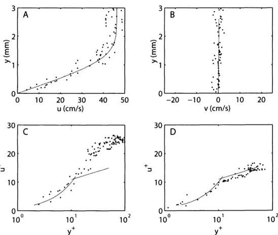
the non-dimensionalized tangential velocity, u+, is plotted as a function of logio(y+). Fig. 2.1A shows the law of the wall plotted in this manner. Two distinct curves are evident. Closest to the wall, which can be thought of as running parallel to the u+axis, the profile is linear, with u+= y+. Note that on a semi-logarithmic plot the relationship does not look linear. This curve represents the linear sublayer, which is commonly referred to as the viscous sublayer in the analysis of turbulent boundary layers. Farther from the wall, the profile follows a logarithmic curve. Flow is turbulent in the logarithmic region and laminar in the linear sublayer; a region called the transition zone separates the two. Unlike the linear sublayer, the shape and position of the logarithmic region of the time averaged profile may very significantly as a result of surface roughness and streamwise pressure gradients (Schetz, 1993). For this reason, data in the logarithmic region cannot be used to determine wall shear stress on an undulating fish. The linear sublayer must be used. Nevertheless, the general shape of the logarithmic region is still useful to

distinguish between turbulent and laminar profiles. Boundary layer profiles were fit to the law of the wall using the linear sublayer when possible. The profile was then classified as turbulent or laminar based on the profile shape outside the linear sublayer. For example, if the Blasius boundary layer is plotted using the non-dimensionalization of Eq. 2.7, the majority of the boundary layer profile follows the linear curve and is poorly fit by the logarithmic curve (Fig. 2.1B).

It should be noted here that for turbulent boundary layers, it is the time-averaged profile at a given streamwise position that is described by the law of the wall. This dependence of the analysis of turbulence on sampling time is due to the fluctuating nature of turbulent flow. If the sampling time is too short, the instantaneous boundary layer profile could appear to be laminar-and not necessarily Blasius-like--even if the flow were turbulent. It is only when several instantaneous boundary layer profiles over a particular point in a turbulent boundary layer are drawn overlapped, that the average curve drawn through the combined profiles follows the law of the wall. Profiles acquired

(32)

30 20 + 10 A 100 101 102 Y 6U

20

+ 10 Aq 100 101 102 Y

Fig. 2.1 Tangential boundary layer profiles presented as is conventional for the law of the wall. u+ and y+ are non-dimensionalized tangential velocity and normal distance from the body surface. (A) The time-averaged profile of the law of the wall for turbulent boundary layer flow over a flat plate with no streamwise pressure gradient plotted in non-dimensional wall units on a semi-logarithmic graph. (B) The tangential velocity profile of the laminar, zero streamwise pressure gradient, flat plate Blasius boundary layer, 'o', scaled as for the law of the wall. The values used for velocity, U, streamwise position, x, and temperature, T, are within the

experimental ranges of the present work.

(33)

by PIV from individual image pairs, at most, can be considered time averages over an effective sampling period of Ts = T/U, where t is the streamwise dimension of the field of view and U is the swimming speed. T in the experiments reported here ranged from 0.01 -- 0.1 s, much shorter than traditional sampling periods. This leads to uncertainty in the designation of certain profiles as turbulent unless several boundary layers at the same swimming speed, body position and body phase are acquired. Nevertheless, several fish boundary layer profiles at high Reynolds numbers showed excellent agreement with the law of the wall. More importantly, in the neighborhood of a particular surface position, the shapes of u-profiles in the linear sublayer of a turbulent boundary layer are less variable than those in the logarithmic region. Therefore, measurements of wall shear stress based on the linear sublayer, are accurate regardless of proper characterization of the boundary layer as matching a known profile shape.

2.5 The 1/7th power turbulent boundary layer profile approximation

It can be shown that an equation of the form

u(y) = o0yl /₇ _(2.9)

is a reasonably good approximation for the tangential profile of a turbulent boundary layer over a flat plate with no streamwise pressure gradient. The law of the wall is better overall, but the 1/7th power profile allows for a set of simple equations regarding &99 and

ro to be written, as for Blasius,

99 = 0.373xRe'/ 5

(2.10)

r

o= 0.0290pU 2Rel'"5

(34)

These equations are used frequently in this investigation for simple comparisons related to turbulent boundary layers.

2.6 Turbulence intensity

The intensity of turbulence in the freestream flow affects the boundary layer over an object. The definition of turbulence intensity in a flow starts with separating the flow into the sum of a mean flow an each position r in the flow, i.e. U = U(r), and a fluctuating component, u' = u'(r,t). Each component of the velocity, U, V and W, can be similarly treated. Turbulence intensity for the x-direction is defined as

I._ (9 1 1

x

Ux-.

where each ti represents a time of sampling of the fluctuating velocity component u', n is the total number of samples, and Uo is usually the overall mean freestream flow speed (Patton, 1984). This is simply the root-mean-square (RMS) of u' divided by the mean freestream flow. Overall turbulence intensity includes all three velocity components and is defined

1 , ([' (r ti)

+

[v(r,

ti)]

+

[w(r, ti)]

2

₎

I -n (2.12)

Uo

Turbulence intensity has a major impact on the value of the critical Reynolds number in boundary layer flow, i.e. the Reynolds number at which the boundary layer transitions to

(35)

turbulence. Theory predicts a critical Rex of -2.5 x 106 for turbulence intensity close to 0. As a rule of thumb however, a critical Rex of 3.5 x 105to 5 x 105 is commonly reported for boundary layer transition. This range is that predicted for a freestream turbulence intensity of 1 - 2% by the theory of Van Driest and Blumer (1963). This is the turbulence intensity commonly found in good quality flumes.

2.7 Boundary layer thickness

As mentioned in the Introduction (section 1.1), since u(y) in the boundary layer approaches the external flow velocity, Ue, asymptotically, boundary layer thickness is commonly defined as the height above the surface at which u = 0.99Ue. This quantity is given the symbol, &99. In this thesis, another boundary layer thickness, &95, defined at u = 0.95Ue is used. Standard deviation in flow velocities within the boundary layer was generally close to 1%, thus automatic determination of the position 0.95Ue was more robust. The Blasius boundary layer equation for 695 is

695 = 3.9xRe"1/2. (2.13)

Eqs. 2.3 and 2.13 show, that regardless of how it is defined, &95 or d, boundary layer thickness grows as x1/2. Eq. 2.10 shows that a turbulent boundary layer tends to grow faster, i.e. as x 4/5.

2.8 Wall shear stress and friction drag

Wall shear stress, and therefore skin friction, can be determined from tangential boundary layer velocity profiles. In the u-direction, the component of wall shear stress,

(36)

y=u

T = U,

au

(2.14)

where ,u is the dynamic viscosity of the fluid, u = u(y) is the tangential component of fluid velocity over the object in the x-direction, and y is in the direction of the local outward normal of the surface. In the linear sublayer of both laminar and turbulent boundary layers, the instantaneous value of the partial derivative-the normal gradient of u-at the body surface can be determined by a simple linear fit depending on the

resolution of the flow. This use of experimental data to determine wall shear stress has been termed the 'near-wall method' by Osterlund and Johansson (1999). Their wall shear stresses calculated from Eq. 2.14 using hot-wire velocity measurements show excellent agreement with theory and concurrent measurements of shear stress by the oil film technique (Siller, et al., 1993). They also determined and verified fluctuating shear stress measurements, due to the unsteadiness of turbulent flow, with MEMS-type hot films.

The wall shear stress distribution, o,, over an object can be used to calculate the total friction drag, Df, using,

D, = fro dA cosO (2.15)

S

where S is the three-dimensional function defining the body surface of the fish, dA is the incremental area over which a particular shear stress applies, and O is the angle between the body surface tangent in the laser plane and the streamwise direction. The coefficient of friction for any object is defined as,

D=

C -pAU 2 (2.16)

2

(37)

where p is the fluid density, A is the total wetted surface area of the body, and U is the relative velocity of the object through the fluid. In order to obtain accurate values of friction drag and the coefficient of friction for a swimming fish, a large number of measurements of wall shear stress at different positions and at different phases of the undulatory motion must be taken.

For comparison purposes, a local coefficient of friction, Cfx, was defined as,

T.,o(X)

Cfx

U

2

_(2.17)

pU

By this definition, Cf is the area average of Cfx over the fish surface. Therefore, Cf for a given fish falls between the maximum and minimum values of Cfx determined over the fish body. Both time averaged and instantaneous values of Cfx were examined.

(38)

(39)

Chapter 3 Preliminary investigation

This chapter is an abridged version of the Methods and Materials, Results and Discussion from the paper titled 'The boundary layer of swimming fish' published in the Journal of Experimental Biology by the author, W. R. McGillis, and M. A. Grosenbaugh (Anderson et al., 2001a). The paper describes the successful visualization of the fish boundary layer by a highly manual data acquisition and analysis system.

3.1 Methods and materials

3.1.1 Fish

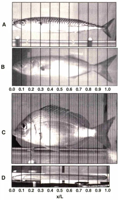
Scup, Stenotomus chrysops, (n = 9) and smooth dogfish, Mustelus canis, (n = 1), were caught in traps or by hook and line in Nantucket Sound, off Woods Hole, MA, USA. The animals were kept in 750-liter tanks with a constant flow of fresh seawater from Nantucket Sound. All fish kept longer than 2 days were fed a steady diet of frozen squid. Fish were transferred to and from their tanks in 30-liter buckets or 60-liter coolers. Following experiments, fish were euthanized by cervical transection according to the WHOI Institutional Animal Care and Use Committee (IACUC) protocol at the time of the experiments. The body length, L, of scup averaged 19.5 ± 1.8 cm (mean ± S.D.). The dogfish measured 44.4 cm.

3.1.2 Swimming conditions

Scup were observed swimming in both still water and in a flume. In still water, scup were observed swimming 3 - 40 cm s-' at water temperatures of 11 C or 22 - 25 C,

(40)

depending on the season during which the experiments were run. In the flume, scup were observed swimming 10 - 65 cm s-1 at 22 - 23 C. The dogfish was observed swimming 20 - 65 cm s in the flume at 22 - 23 C.

In flume trials, observations from three positions along the midline of each fish were performed at one or more speeds. In scup, the measurements were made at x = 0.50L, 0.77L, and 0.91L. In dogfish, the measurements were made at x = 0.44L, 0.53L, and 0.69L. The majority of flume data for scup was acquired at swimming speed 30 cm

S-' (18 swimming sequences). At this speed, scup were observed to use primarily caudal

fin propulsion with infrequent strokes by their pectoral fins. Records of transverse velocity showed continuous undulatory swimming during all acquired sequences. In still water, scup tended to swim more slowly, frequently using their pectoral fins and gliding. Therefore, in our analysis of the fish boundary layer, we have concentrated on the flume experiments and the fastest of the still water swimming sequences. The majority of the flume data for the dogfish was acquired at the swimming speed 20 cm s-1 (22 swimming sequences). Rigid-body measurements in dogfish were made at two positions, x = 0.44L and 0.69L at 20 cm s-. The more forward positions on the dogfish were chosen because it was difficult to acquire sufficient data in the posterior region where the body wave amplitude increases dramatically with position. At positions posterior to x = 0.75L, the fish surface was captured infrequently in the small field of view of the flow-imaging camera. The swimming speeds of 30 cm s-1in scup and 20 cm s-1 in dogfish were chosen because at these speeds the fish swam steadily for long periods of time without tiring.

Still water trials were performed in a large rectangular tank (2.5 m x 1.2 m x 0.5 m). Water depth was 20 cm. A channel, 20 cm wide, was constructed along one of the long glass walls of the tank. The midpoint of the channel was used as the test section. The flow-imaging camera was partially submerged in a glass enclosure to prevent free surface optical distortion. Fish swam deeply and slowly enough so that free surface wave effects were negligible. Flowing water trials were performed in a large, recirculating,

(41)

open-channel flume capable of speeds up to 70 cm s'l. The racing oval shaped flume, with straight-aways 7.6 m long, is paddle driven by a conveyor belt mechanism. The flume channel is 78 cm wide and 30 cm deep. Water depth during fish swimming trials was 16 cm. The test section used was constructed against one of the glass walls of the flume, 20 cm wide and 80 cm long. The free surface was eliminated using a sheet of acrylic. Honeycomb flow-through barriers bound the test section, confining the fish to the test section, and damping out large-scale flow disturbances. The barriers were 12.7 cm in streamwise length with tube diameter of 1.3 cm. Turbulence intensity in the test section measured by laser Doppler anemometry, LDA, was 4 - 6% over the range of experimental flow speeds. Without the honeycomb barriers, turbulence intensity measured 7 -- 8%. Velocity measurements outside of the fish boundary layer

demonstrated scatter in agreement with the measured test section turbulence intensity. Still water trials showed little to no scatter in velocity outside the boundary layer. In both still and flowing water trials, fish swam far enough from the wall on the side of the fish measured-generally 8 - 12 cm--that wall effects are expected to be minimal.

3.1.3 Image acquisition

Fluid flow around the fish was illuminated by a horizontal laser sheet, 0.5 mm thick, and imaged from above with a high-resolution digital video camera (Kodak ES 1.0,

1008 pixels x 1018 pixels)-the 'boundary layer camera' shown in Fig. 3.1. The second camera shown above the test section in Fig. 3.1, the 'nearfield camera' was added in the advanced study (see Chapter 4). The flow was seeded with neutrally buoyant fluorescent particles, 20 - 40 gm in diameter. Macro photographic lenses (Nikon, Micro-Nikkor, 60mm) were used to obtain high quality, high magnification images of particles in the flow over the fish surface (Fig. 3.2). Fields of view used with the particle imaging camera were 1 - 2 cm on a side. The resulting images had a scale of 50 - 100 pixels mml'. Our fish boundary layers measured 0.5 - 12 mm in thickness. The laser (New Wave Research, Nd:YAG, dual pulsed) was operated at low power to prevent irritation to

(42)

Boundary layer Camera Nearfield Camera

Fig.3.1 Sketch of the setup for boundary layer visualization. The bright line on the fish centerline shows where the laser impinges on the fish surface. The nearfield camera was added after the preliminary investigation. The boundary layer and nearfield cameras were also moved underneath the test section. See text for information about the variety of barriers used to constrain the fish to the test section.

(43)

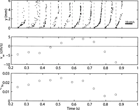
Fig. 3.2 A double exposure showing examples of particle pairs used to determine fluid velocities in the boundary layer around a swimming scup. A particle pair is labeled with white arrows. The particles in the image were moving roughly left to right. Scale bar is 1 nun. The camera angle was as shown in Fig. 3.1 (the boundary layer camera). The body surface of the scup appears as a sharp, bright edge in the lower half of the image. The position on the scup shown isx

=

O.55L on the midline of the fish. The scup was swimming 8.3 cm S-1through still water, roughly to the right in the field of view (black

arrow). The body surface was moving laterally 1.7 cm s-J in the direction away from the region of fluid shown here in the upper portion of the image. Note that the particles closer to the fish move a greater distance than particles further away from the fish. This is because the fluid closest to the fish is influenced most by the motion of the fish through the fluid. However, in the frame of reference of the fish, the particles closest to the fish are moving more slowly than the particles further from the fish, resulting in boundary layer profiles similar to those shown in Fig. 1.1. The double exposure was constructed simply by adding successive video images. The image was swept of approximately half of its original particles and threshold filtered for clarity of presentation.

(44)

the animal and to minimize glare. The time delay, At, between laser pulses, i.e. between exposures of the flow, was set at 2 - 10 ms depending on swimming speed. The

measured displacement of particles between exposures is divided by this time to obtain particle velocities. The laser and the particle imaging camera were synchronized using a digital delay triggered by every other vertical drive signal of the camera. The vertical drive signal is a TTL pulse that signals the moment between two exposures. When triggered, the digital delay triggered laser 1 of the dual laser to fire At/2 before, and laser 2 to fire At/2 after, the next vertical drive signal of the camera, which was 'ignored' by the digital delay. The camera was operated at approximately 30Hz and 100 sequential images were acquired per swimming sequence. Therefore, pairs of exposures, or image pairs, were acquired at 15 Hz, and continuous sequences of 50 pairs were acquired. Two

standard video cameras were used to obtain simultaneous records of whole body motion in lateral and dorsal views. This allowed fish boundary layer flow to be compared with relevant instantaneous whole body kinematic parameters.

Measurements were confined to positions on the fish where the body surface was essentially perpendicular to the laser sheet. As the angle between the laser sheet and the fish surface deviates from 900, boundary layer velocity profiles are distorted, tending to give an incorrectly low wall shear stress. Images in which the fish surface is

perpendicular to the laser sheet are easily distinguished from images in which the surface is at an angle to the sheet. In the former, the fish surface appears as a sharp edge. In the

latter, depending on the direction of tilt, either the intersection of the beam and the fish surface is not visible, or the features of the fish surface beneath the sheet are visible, dimly illuminated by reflected laser light. Only images of the former type were used in the analysis.

In both still water and flume trials, all three video cameras were fixed with respect to the frame of the test section during image acquisition. In still water, the fish swam through the test section. Therefore they swam through each camera's field of view at

(45)

their swimming speed, U, and flow velocity outside the fish boundary layer was nearly zero. In the flume, fish held station in the test section without significant streamwise motion with respect to the fields of view. The flow outside the boundary layer of the fish therefore moved through the fields of view at the approximate flume speed, U. Apart from the ambient turbulence of the flume flow, the two situations are equivalent from the standpoint of fluid dynamics. Both techniques proved useful to the analysis of the fish boundary layer. Still water trials revealed actual boundary layer development over particular fish in undisturbed flow, whereas flume trials revealed the phase dependent aspects of the boundary layer at selected positions on the fish. The flume was also used to look at boundary layer development by recording several sequences from various streamwise positions.

3.1.4 Rigid-body drag

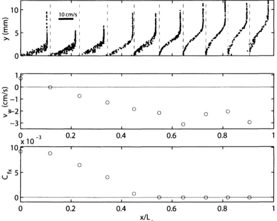
In general, the dogfish swam very close to the bottom of the flume, and it was possible to measure the boundary layer of the dogfish at the same streamwise position and flume speed for both swimming and resting. Three image sequences of the dogfish boundary layer were acquired while the dogfish conveniently rested motionless on the bottom of the flume. The flume speed and water temperature were 20 cm s and 23 c. The resting data were used to determine rigid-body friction drag for the dogfish.

It was important to confirm that the bottom boundary layer of the test section did not affect the rigid-body measurements significantly. LDA showed that the boundary layer of the test section bottom was thinner than 1.5 cm. Dogfish boundary layer data was taken between 1.2 - 1.8 cm. Flow visualizations were therefore made outside, or at the outer edge of the flume bottom boundary layer, where small changes in the height would not be expected to have a significant effect on the flow velocities at the outer edge of the boundary layer, Ue. Velocities measured by particle tracking confirmed this. Ue in

(46)

both the swimming and rigid-body cases was found to be essentially the same at x = 0.44L.

3.1.5 Digital particle tracking velocimetry

The acquisition and analysis of image pairs for digital particle imaging

velocimetry, DPIV, and digital particle tracking velocimetry, DPTV, is now common practice among engineers, chemists and a growing number of biologists. For this reason the details of these techniques will be left to the numerous existing works on the subject; the reader is referred to Adrian (1991), Willert and Gharib (1991) and Stamhuis and Videler (1995). Here, we report the variations on the themes of DPIV and DPTV

necessary to capture and resolve the fish boundary layer. Flow velocities around the fish were quantified primarily by semi-automatic DPTV (Stamhuis and Videler, 1995). Particle pairs are located manually with a cursor on the computer screen. The term 'particle pair' refers to the two images of the same particle that occur in an image pair. A particular image pair typically has tens to hundreds of particle pairs depending on seeding density. Once the particle pairs have been located, a computer program then determines the centroids of the particles and calculates displacement and velocity. Conventional DPIV and automatic particle tracking code were sometimes used to resolve the outermost regions of boundary layer flow, but they often failed to resolve the flow very close to the moving surface of the fish.

The fish surface was located using an edge detection algorithm developed in the study of squid locomotion (Anderson and DeMont, 2000; Anderson et al., 2001b). The algorithm was further developed in the course of the present work to match surface features in sequential images and thereby calculate the precise motions of the animal surface. This motion was conveniently described by a tangential and normal

displacement. Deformation and rotation of the fish surface was found to be negligible for any image pair due to the short time separating the images and the small field of view.

(47)

Trials during which the fish rested motionless on the bottom of the tank revealed the accuracy of this wall-tracking algorithm to be better than 0.5 pixels. At our

magnifications, this represents 10 - 20tm error in displacement and, after smoothing, negligible error in surface slope. For a typical swimming trial, say U = 20 cm s-1 and At = 5 ms, this translates to less than 2% error in the measurement of tangential flow velocity relative to the fish surface. Average maximum error in normal velocity is 2 -10%, depending on the magnitude of the transverse body velocity. Since wall shear stresses were determined from the slope of the boundary layer profile near the body surface, such errors in velocity relative to the fish surface do not affect our calculated skin friction.. Instead, these errors impact less critical measurements, such as outer edge velocity, boundary layer thickness, and their fluctuations. In general, these parameters were large enough that errors were insignificant to negligible.

3.1.6 Tangential and normal velocity calculations

To construct tangential and normal velocity profiles from the image pairs of flow over the fish surface, the motion of particles in the image pairs must be viewed from the reference frame of the fish. Unless the surface can be described by a straight line, this requires the construction of axes normal and tangential to the fish surface for each particle. Assuming the velocity profiles do not change significantly over the relatively small field of view, this method results in the desired boundary layer profiles. The separate profiles are built up from the normal and tangential components of velocity determined for each particle, with respect to the fish, plotted against normal distance of the particle from the fish surface.

Normals from particles to the fish surface were determined though a standard minimization of the distances from the particles to the fish surface. The radius of curvature of the fish surface was always larger in scale than the field of view. This ensured convergence of the minimization process. The fish body surface was found to be