LEVERAGING SOFTWARE CLONES FOR SOFTWARE COMPREHENSION: TECHNIQUES AND PRACTICE
THIERRY M. LAVOIE
D´EPARTEMENT DE G´ENIE INFORMATIQUE ET G´ENIE LOGICIEL ´
ECOLE POLYTECHNIQUE DE MONTR´EAL
TH`ESE PR´ESENT´EE EN VUE DE L’OBTENTION DU DIPL ˆOME DE PHILOSOPHIÆ DOCTOR
(G´ENIE INFORMATIQUE) AVRIL 2015
c
LEVERAGING SOFTWARE CLONES FOR SOFTWARE COMPREHENSION: TECHNIQUES AND PRACTICE
pr´esent´ee par: LAVOIE Thierry M.
en vue de l’obtention du diplˆome de: Philosophiæ Doctor a ´et´e dˆument accept´ee par le jury d’examen constitu´e de:
M. FERNANDEZ Jos´e M., Ph. D., pr´esident
M. MERLO Ettore, Ph. D., membre et directeur de recherche M. ADAMS Bram, Doctorat, membre
Tout d’abord, pour sept ann´ees r´eparties sur trois cycles et un nombre incalculable de projets et d’opportunit´es, je remercie le Professeur Ettore Merlo, directeur et mentor, de m’avoir accord´e autant de libert´e, de confiance et de d´efis et de m’avoir autant ´epaul´e et encourag´e. Ce fˆut, et je l’esp`ere sera, un immense plaisir de vous avoir connu et d’avoir travailler pour et avec vous.
Je remercie mes parents, Murielle et Daniel, de m’avoir soutenu `a travers le parcours le plus difficile qui soit. Je vous le promets, cette fois-ci je quitte d´efinitivement l’universit´e.
`
A ma soeur et `a mon beau-fr`ere, Maryse et Jean-Philippe, merci de m’avoir offert une vie comprise de 1000km de course et de poros. Votre accompagnement a ´et´e appr´eci´e. Merci aussi `a ces amiti´es que vous avez partag´ees: Dave, Mr. Phil et Antoine.
Merci `a mes coll`egues de laboratoire, Mathieu et Marc-Andr´e. Je vous souhaite `a votre tour d’atteindre cette ´etape.
Un merci sp´ecial `a Pascal Potvin et son ´equipe, Mario, Marco, Gordon et Renaud de chez Ericsson pour m’avoir offert une chance unique d’avoir une exp´erience industrielle lors de mon passage `a l’universit´e. Votre influence m’a donn´e le goˆut de cette aventure.
Et finalement, `a cinq grandes amiti´es.
Fran¸cois, tu as ´et´e ce coll`egue qui fait de l’universit´e ce qu’elle doit ˆetre: un lieu de haut ´echange intellectuel. J’ai ´et´e honnor´e de travailler avec toi et de partager autant de jeux de soci´et´e.
Elyse, merci d’avoir ´et´e l`a, merci d’avoir march´e avec moi, merci pour les gˆateaux, merci pour les projets un peu fou, de 20kg de pommes `a la neige de l’Estrie jusqu’aux hanches, merci pour tout, tout simplement.
Sag, merci de m’avoir rappel´e qu’il faut d´ecrocher et garder les pieds sur terre.
Th´eotime, merci d’avoir ´et´e aussi joyeux et de m’avoir ouvert l’esprit un peu plus sur le monde.
Am´elie, merci d’ˆetre cette constante dans ma vie qui me rappelle que les choses reviennent toujours `a l’´equilibre.
`
Additional Acknowledgements
This research was funded by NSERC, FQRNT, and Ericsson Canada. Chapters 1, 2, 3, 5, 11, 12, and 13 were proofread by Ivanna Richardson.
Chapter 11 contains results on which the following people have contributed: Ettore Merlo, Pascal Potvin, Pierre Busnel, Gordon Bailey, Fran¸cois Gauthier, and Jean-Fran¸cois Li. They all gave their explicit consent to the use of some figures and text presented in that chapter. Ettore Merlo, Pascal Potvin, and Fran¸cois Gauthier also gave many comments that helped shape the discourse of that chapter.
librairie impl´emente un arbre de m´etrique g´en´eral, une structure de donn´ee sp´ecialis´ee dans la division des espaces de m´etriques dans le but d’acc´el´erer certaines requˆetes communes, comme les requˆetes par intervalles ou les requˆetes de plus proche voisin. Cette structure est utilis´ee pour construire un d´etecteur de clones qui approxime la distance de Levenshtein avec une forte pr´ecision. Une br`eve ´evaluation est pr´esent´ee pour soutenir cette pr´ecision. D’autres r´esultats pertinents sur les m´etriques et la d´etection incr´ementale de clones sont ´egalement pr´esent´es.
Plusieurs applications du nouveau d´etecteur de clones sont pr´esent´es. Tout d’abord, un algorithme original pour la reconstruction d’informations perdus dans les syst`emes de version-nement est propos´e et test´e sur plusieurs grands syst`emes. Puis, une ´evaluation qualitative et quantitative de Firefox est faite sur la base d’une analyse du plus proche voisin; les courbes obtenues sont utilis´ees pour mettre en lumi`ere les difficult´es d’effectuer une transition entre un cycle de d´eveloppement lent et rapide. Ensuite, deux exp´eriences industrielles d’utilisation et de d´eploiement d’une technologie de d´etection de clonage sont pr´esent´es. Ces deux exp´eri-ences concernent les langages C/C++, Java et TTCN-3. La grande diff´erence de population de clones entre C/C++ et Java et TTCN-3 est pr´esent´ee. Finalement, un r´esultat obtenu grˆace au croisement d’une analyse de clones et d’une analyse de flux de s´ecurit´e met en lumi`ere l’utilit´e des clones dans l’identification des failles de s´ecurit´e.
ABSTRACT
This thesis explores two topics in clone analysis: detection and application.
The main contribution in clone detection is a new clone detector based on a library called mtreelib. This library is a package developed for clone detection that implements the metric data structure. This structure is used to build a clone detector that approximates the Levenshtein distance with high accuracy. A small benchmark is produced to assess the accuracy. Other results from these regarding metrics and incremental clone detection are also presented.
Many applications of the clone detector are introduced. An original algorithm to recon-struct missing information in the recon-structure of software repositories is described and tested with data sourced from large existing software. An insight into Firefox is exposed showing the quantity of change between versions and the link between different release cycle types and the number of bugs. Also, an analysis crossing the results from pattern traversal, flow analysis and clone detection is presented. Two industrial experiments using a different clone detector, CLAN, are also presented with some developers’ perspectives. One of the experi-ments is done on a language never explored in clone detection, TTCN-3, and the results show that the clone population in that language differs greatly from other well-known languages, like C/C++ and Java.
The thesis concludes with a summary of the findings and some perspectives for future research.
R´ESUM´E . . . vi
ABSTRACT . . . vii
CONTENTS . . . viii
LIST OF TABLES . . . xii
LIST OF FIGURES . . . xiv
LIST OF SYMBOLS ET ABREVIATIONS . . . xvi
CHAPTER 1 INTRODUCTION . . . 1
1.1 Basic Concept Definitions . . . 1
1.1.1 Definition of Clone Types . . . 1
1.1.2 Definition of Similarity and Distance . . . 2
1.2 Problem Definitions and Research Objectives . . . 3
1.2.1 Accurate Clone Detection using Metric Tree, n-grams, and Non-Euclidean Metrics . . . 3
1.2.2 Exploring New Applications of Clone Detection Technology . . . 4
1.2.3 Contributions . . . 4
CHAPTER 2 LITERATURE REVIEW . . . 5
2.1 Clone Detection . . . 5
2.2 Approximate String Matching . . . 6
2.3 Clone Management and Applications . . . 7
2.4 Clone Evaluation . . . 8
CHAPTER 3 TECHNICAL IMPLEMENTATION, PRELIMINARY CONSIDERATIONS, AND RESEARCH OVERVIEW . . . 9
3.1 Implementation Of mtreelib . . . 9
CHAPTER 4 PAPER 1: AN ACCURATE ESTIMATION OF THE LEVENSHTEIN
DISTANCE USING METRIC TREES AND MANHATTAN DISTANCE . . . 12
4.1 Abstract . . . 12
4.2 Introduction . . . 12
4.3 Literature Review . . . 13
4.4 Algorithm . . . 14
4.5 Experiments and Results . . . 19
4.6 Discussion . . . 25
4.7 Conclusion . . . 28
CHAPTER 5 ERRATA AND COMMENTS ON PAPER 1 . . . 29
CHAPTER 6 PAPER 2: ABOUT METRICS FOR CLONE DETECTION . . . 31
6.1 Introduction . . . 31
6.2 An Equivalence of the Jaccard Metric and the Manhattan Distance . . . 31
6.3 Properties of Some Angular Distances . . . 33
6.4 Further Questions and Research: Implicit Distances, Why Should we Recover them ? . . . 35
CHAPTER 7 PAPER 3: PERFORMANCE IMPACT OF LAZY DELETION IN MET-RIC TREES FOR INCREMENTAL CLONE ANALYSIS . . . 37
7.1 Abstract . . . 37 7.2 Introduction . . . 37 7.3 Methodology . . . 38 7.4 Results . . . 39 7.5 Discussion . . . 41 7.6 Related Works . . . 43 7.7 Conclusion . . . 44
CHAPTER 8 COMMENTS ON PAPER 3 . . . 45
CHAPTER 9 PAPER 4: HOW MUCH REALLY CHANGES? A CASE STUDY OF FIREFOX VERSION EVOLUTION USING A CLONE DETECTOR . . . 46
9.1 Abstract . . . 46
9.2 Introduction . . . 46
9.3 Methodology . . . 47
9.4 Results . . . 49
CHAPTER 11 PAPER 5: TTCN-3 TEST SUITES CLONE ANALYSIS IN AN
INDUS-TRIAL TELECOMMUNICATION SETTING . . . 63
11.1 Abstract . . . 63
11.2 Introduction . . . 63
11.3 Adapting Clone Technology For TTCN-3 . . . 65
11.4 Experiments . . . 66
11.4.1 Experimental Setup . . . 66
11.4.2 TTCN-3 Results . . . 68
11.4.3 Statistical analysis . . . 71
11.5 Discussion and Lessons Learned . . . 74
11.6 Related Work . . . 76
11.6.1 Applications in large-scale and industrial context . . . 76
11.6.2 Summary of Different Clone Detection Techniques . . . 77
11.6.3 Parsing Techniques . . . 78
11.6.4 Applications . . . 79
11.7 Further research . . . 79
11.8 Conclusion . . . 80
CHAPTER 12 PAPER 6: INFERRING REPOSITORY FILE STRUCTURE MODIFI-CATIONS USING NEAREST-NEIGHBOR CLONE DETECTION . . . 81
12.1 Abstract . . . 81
12.2 Introduction . . . 81
12.3 Literature . . . 82
12.3.1 Clone Detection Techniques . . . 82
12.3.2 Provenance and Clone Evolution Analysis . . . 83
12.4 Problem, Algorithm, and Method . . . 83
12.4.1 Definition of the problem . . . 83
12.4.2 Metric tree definition and construction . . . 84
12.4.4 Using a Nearest-Neighbor approach . . . 90
12.5 Experimental setup . . . 91
12.5.1 Analyzed systems and computational equipment . . . 91
12.5.2 Computing the nearest-neighbor . . . 95
12.5.3 Building the repository oracle using VCSMiner . . . 95
12.5.4 Categorizing the oracle moves . . . 96
12.5.5 Methodology to compute precision and recall . . . 96
12.6 Results . . . 96
12.7 Discussion . . . 99
12.7.1 Threats to validity . . . 103
12.8 Conclusion . . . 104
12.9 Acknowledgments . . . 105
CHAPTER 13 ADDITIONAL RESULTS AND APPLICATIONS . . . 106
13.1 Clones In A Large Telecommunication Industrial Setting . . . 106
13.1.1 Experiments . . . 106
13.1.2 C/C++ Results . . . 109
13.1.3 JAVA Results . . . 113
13.1.4 Discussion and Lessons Learned . . . 113
13.1.5 Industrial perspectives . . . 114
13.1.6 Academic perspectives . . . 121
13.2 Security Discordant Clones . . . 122
13.2.1 Identified Security flaws . . . 124
CHAPTER 14 GENERAL DISCUSSION . . . 129
14.1 Discussion on The Techniques for Clone Detection . . . 129
14.2 Discussion on Applications of Clone Detection . . . 130
14.3 General Observations and Closing Comments . . . 131
CHAPTER 15 CONCLUSION . . . 132
Table 4.3 Tomcat optimal F-value for fixed Levenshtein distance and window length. Values in table are formatted as (radius,F-value,clones
num-ber). Radii are relative values. . . 27
Table 4.4 Tomcat precision and recall values for best achievable F-value . . . 27
Table 4.5 Execution time of the Levenshtein oracle compared to the configuration for best results with Manhattan . . . 27
Table 7.1 Details of Firefox 17 versions. Methods of interest are only those of size greater than 100 tokens. . . 40
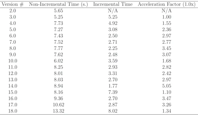
Table 7.2 Execution time of metric tree clone detection at distance 0.0 for non-incremental and non-incremental clone detection in Firefox versions . . . . 42
Table 7.3 Execution time of metric tree clone detection at distance 0.1 for non-incremental and non-incremental clone detection in Firefox versions . . . . 42
Table 9.1 Details of Firefox 18 versions. Methods of interest are only those of size greater than 100 tokens. . . 50
Table 9.2 Summary of changes between versions. Relative values are relative to the total number of methods in the preceding version. . . 52
Table 11.1 Sizes of Test Script Sets . . . 67
Table 11.2 All systems clone clustering and DP computation time . . . 67
Table 11.3 TTCN Detailed Clone Clustering . . . 69
Table 11.4 Example of a contingency table . . . 72
Table 11.5 Contingency table for TTCN and C/C++ . . . 73
Table 11.6 Contingency table for TTCN and Java . . . 73
Table 12.1 Criteria for region selection in the findnn primitive. . . 91
Table 12.2 Systems versions statistics . . . 94
Table 12.3 JHotDraw recall of inferred moves, with implicit found moves. . . 97
Table 12.4 Tomcat recall of inferred moves, with implicit found moves. . . 98
Table 12.5 Adempiere recall of inferred moves, with implicit found moves. . . 98
Table 12.6 Average similarity of True Move and Implicit Move for all systems . . . 99
Table 13.2 Features . . . 107 Table 13.3 Computation times for each step of the analysis together with numbers
of privileges and PHP lines of code. . . 123 Table 13.4 Numbers of novel and known access control flaws that were revealed
green curve, 0.2, and red curve 0.1 . . . 20
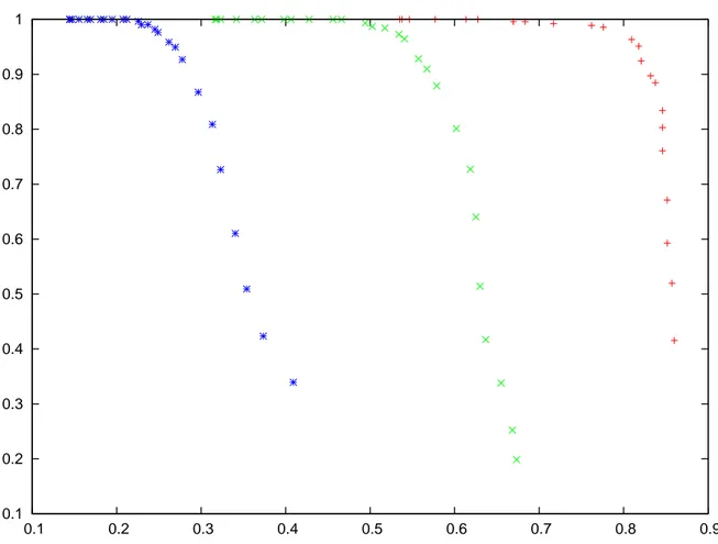
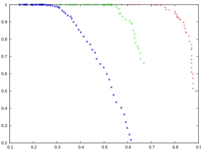
Figure 4.4 Precision with respect to recall for Tomcat and a window length of 2. Radii value on y-axis is relative. Blue curve is for Levenshtein 0.3, green curve, 0.2, and red curve 0.1 . . . 21
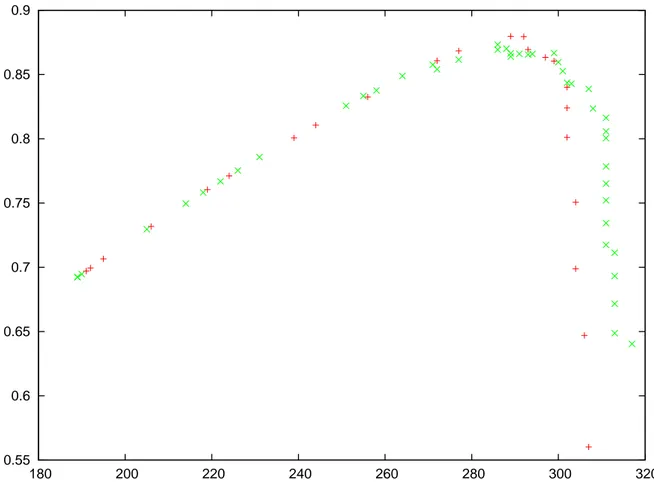
Figure 4.5 F-Value with respect to the total number of accepted clones for Tomcat with a Levenshtein threshold of 0.1. Red curve is for window length 1, green curve is for window length 2 . . . 22
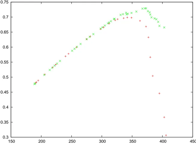
Figure 4.6 F-Value with respect to the total number of accepted clones for Tomcat with a Levenshtein threshold of 0.2. Red curve is for window length 1, green curve is for window length 2 . . . 23
Figure 4.7 F-Value with respect to the total number of accepted clones for Tomcat with a Levenshtein threshold of 0.3. Red curve is for window length 1, green curve is for window length 2 . . . 24
Figure 4.8 Total execution time with respect to query radius in Tomcat. Red curve is for window length 1, green curve is for window length 2 . . . . 26
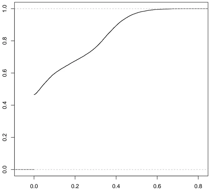
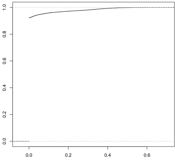
Figure 9.1 Cumulative distribution of the differences between methods of Firefox 3.0 and their respective closest match in Firefox 2.0. . . 53
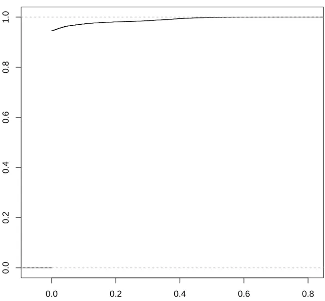
Figure 9.2 Cumulative distribution of the differences between methods of Firefox 7.0 and their respective closest match in Firefox 6.0. . . 54
Figure 9.3 Cumulative distribution of the differences between methods of Firefox 8.0 and their respective closest match in Firefox 7.0. . . 55
Figure 9.4 Cumulative distribution of the differences between methods of Firefox 18.0 and their respective closest match in Firefox 17.0. . . 56
Figure 11.1 Clone detection process with CLAN . . . 68
Figure 11.2 Cluster size distribution . . . 70
Figure 11.3 Fragment size distribution . . . 70
Figure 11.4 Connected histogram of parametric similarity distribution . . . 70
Figure 11.5 Decreasing cumulative curve of parametric similarity distribution . . . 70
Figure 11.7 Decreasing cumulative curve of similarity distribution . . . 71
Figure 12.1 Insertion algorithm in metric trees . . . 86
Figure 12.2 Nearest-neighbor algorithm in metric trees . . . 92
Figure 12.3 Move inference algorithm (MIA) . . . 93
Figure 12.4 Box-plot of distance distribution of inferred moves excluding identical matches for all systems . . . 100
Figure 12.5 Execution time (s.) of the Nearest-Neighbor clone detection for Tomcat with respect to the number of lines of codes in each version . . . 101
Figure 12.6 Execution time (s.) of the Nearest-Neighbor clone detection for JHot-Draw with respect to the number of lines of codes in each version . . . 101
Figure 12.7 Execution time (s.) of the Nearest-Neighbor clone detection for Adem-piere with respect to the number of lines of codes in each version . . . . 102
Figure 13.1 Cluster size distribution . . . 109
Figure 13.2 Fragment size distribution . . . 110
Figure 13.3 Similarity distribution . . . 111
Figure 13.4 Parametric similarity distribution . . . 112
Figure 13.5 Cluster size distribution . . . 114
Figure 13.6 Fragment size distribution . . . 115
Figure 13.7 Similarity distribution . . . 116
Figure 13.8 Parametric similarity distribution . . . 117
Figure 13.9 Ratios of files and PHP lines of code that were reviewed during the investigation of security-discordant clone clusters. . . 126
Figure 13.10 Distribution of security weaknesses in Joomla! and Moodle. Category names were abbreviated for space considerations: Least privilege viola-tion (L.P.V.), Weak encapsulaviola-tion (W.E.), Shaky logic (S.L.), Semantic inconsistency (S.I.) and Missing privilege (M.P.) . . . 127
Figure 13.11 Distribution of the categories of security-discordant clone clusters in Joomla! and Moodle. Category names were abbreviated for space considerations: Least privilege violation (L.P.V.), Weak encapsulation (W.E.), Shaky logic (S.L.), Semantic inconsistency (S.I.), Missing priv-ilege (M.P.), Utility function (U.F.) and Legitimate (L.) . . . 128
LDA Latent Dirichlet Allocation δ Distance function
CHAPTER 1
INTRODUCTION
Clone detection, as fascinating as controversial, is one of the most active fields in software engineering. Originating now more than 20 years ago, it focuses on the detection of similar code in software applications. Whether for plagiarism detection, bug detection, software evolution, software comprehension, or even simple curiosity, this discipline has produced many interesting ideas on how to improve software quality and maintainability.
However interesting the topic is, many problems are still considered unresolved. In the Dagstuhl seminar of 2012 [71], many unsolved issues were identified, but two major problems emerged as being of crucial interest: improving type-3 clone detection and finding useful industrial applications. A further problem has plagued the community for the past decade: the lack of an extensive methodology to evaluate clone detectors.
This thesis aims to provide solutions to the first two problems mentioned above. The main goal of this research is the design of an accurate type-3 clone detector by the means of estimating the Levenshtein distance. To assess the usefulness of the new method, some applications requiring extensive type-3 clone detection are proposed.
This thesis is divided into topics: the rest of the introduction will cover basic definitions and concepts followed by an overview of the research ideas; the second chapter presents a literature review of clone detection and string matching; the third chapter presents an overview of the technique; and the following chapters present published papers on the topics mentioned before. Further research opportunities are presented in the conclusion.
1.1 Basic Concept Definitions
Prior to any further discussion, we define some important concepts relevant to this thesis. 1.1.1 Definition of Clone Types
Providing a clear definition of all the clone types has proven to be a near-impossible task. Simply by analyzing the references provided in this thesis, many discrepancies are easily identified in the many definitions formulated by different authors. Disagreeing does not however argue against common ground shared among many clone definitions: typical clone
we say it is a type-2 inconsistent.
• Type-3: Gapped clones. Those clones part of whose structure is not syntactically identical. This may result from statement modifications, insertions, and deletions. Type-3 clones do not need to be semantically consistent, meaning they may exhibit different functionalities.
• Type-4: Semantic clones. Those clones who share part of their semantic, but may not share any common structural feature.
This thesis focuses on type-3 clone detection. 1.1.2 Definition of Similarity and Distance
First considering code fragments, clones always have at least an indirect reference to the notions of similarity and the dual concept of distance. Most of the clone detectors available today establish cloning relations based on the notion of similarity. Despite the possibility of computing clones with a similarity measure being a very attractive notion, laying strong mathematical foundations to similarity computation using a distance, instead of a direct similarity measure, is often the more elegant and better choice. To understand how these concepts will be used within this work, we will first define them:
• Similarity: A measure aimed at quantifying how many two objects share common structural features. It can be normalized in the interval [0.0, 1.0], 1.0 meaning identical, 0.0 meaning sharing no features at all. In this work, a similarity function is noted φ • Distance: A measure aimed at quantifying how much two objects differ in their
struc-tural features. A distance of 0.0 between two objects means identical objects. Distances are in general not normalized. In this work, a distance function is noted δ.
1Part of the literature now talks about type-4 and higher orders, instead of only type-4. The boundary
surrounding the actual space of type-4 clones being elusive, it is hazardous to define clone types of higher order. Since this thesis focuses on type-3 clones, we do not feel it is appropriate to go further into the debates regarding type-4 clones and will thus only give a general definition of this type
In the case of normalized similarity, it might be tempting to define a distance based on the simple transformation δ = 1− φ. Even though the dual meaning remains, in many cases this transformation results in a distance that does not have strong properties, like satisfying the axioms of a metric: hence the need to define the function as a distance first.
A remarkable group of distance functions called metrics are well-behaved functions defin-ing a topology over a space and give rise to structures prone to optimization. Most of them by nature are not normalized and defining their exact similarity function counterpart is some-times not trivial. Nevertheless, it is not necessary to define a dual function to interpret the results of a distance function in the context of similarity measures. It is sufficient to define the similarity criteria in terms of distances. For example, a large amount of similarity be-tween objects translates to those objects being separated by a small distance. Thus, even if the literature usually defines clones in term of similarity, we will use the concept of distance instead to define clones. However, as we clearly showed the two concepts to be intertwined, we will say that code fragments are similar whenever we intend to say that they are separated by a (arbitrary) small distance if the context is not ambiguous.
1.2 Problem Definitions and Research Objectives
1.2.1 Accurate Clone Detection using Metric Tree, n-grams, and Non-Euclidean Metrics
Predating the other objective, the design of the new clone detector will be oriented towards an accurate approximation of the Levenshtein distance. There are two reasons to approxi-mate the Levenshtein distance. First, the distance gives clone results of good quality. Second, while the results are good, the computation time is prohibitive. Thus, designing an approxi-mation that preserves as much quality of the original distance as possible while reducing the computational cost is an interesting goal.
The key features of the tool are: the use of n-grams to interpret code fragments as frequency vectors, the use of different metrics to induce a topology on the vector space instead of an arbitrary similarity measure, and space partition and pruning by means of the metric tree to speed up the actual search for clones. Comparison of an extensive collection of clones against the oracle by the Levenshtein distance will be used to quantify and validate the accuracy. Curves showing the behavior of the error with respect to the distance are also provided. This is the first work to actually show the error curves. While the error cannot be lower than O(logn) in general, it tends to be smaller for the approximation of smaller distances, and grows as the approximated distance grows. The curves thus provide further empirical results to enhance the theoritical fundation behind the approximation of
compared to clones in general software. Additional results from clones in large industrial software and results obtained from cross-analysis of clones and security patterns are also presented.
This topic will be presented in detail in chapter 9, chapter 11, chapter 12, and chapter 13.
1.2.3 Contributions
This thesis is centered on work that has generated many other contributions, not limited to published papers. Here is the exhaustive list of those contributions:
• A total of 12 papers, cited 52 times according to Google Scholar.
• A robust implementation of the metric tree data structure, written in C++ and dis-tributed under the BSD-4 clauses license.
• A robust parser for the PHP language.
• An accurate approximation of the Levenshtein distance, along with curves showing the behaviour of the error with respect to the distance.
• Seminal work on two languages never considered for clones: PHP and TTCN.
• The technique presented in chapter 4 was used as a mean of identifying intellectual property violations in a trial. This work was done at the request of Smart&Biggar, and under the supervision of Professor Ettore Merlo, who acted as the expert witness.
CHAPTER 2
LITERATURE REVIEW
The software engineering literature about clone detection, management, application, and evaluation is both well established and extensive. For close to 25 years researchers have contributed to this field and yet many problems are still open. This section presents a broad coverage of the literature. It is divided according to four main topics: clone detection, clone management, clone application, and clone evaluation. Some open problems are also highlighted. Additional references are provided in each paper for the relevant related work.
2.1 Clone Detection
Clone detectors are classified according to their paradigm. We summarize each of these paradigms with key related publications.
Token based clone detectors are among the most primitive clone detectors. Authors such as Kamiya [60], Jarzabek [20], Juergens [58], and Murakami [91] have proposed different variations of this paradigm. Most of the token based approaches use different flavors of hashing to identify clones. They also are agnostic of the syntactic structures because they only use a lexer and no parsing to identify structural boundaries. These clone detectors are relatively easy to implement, but they offer poor results when dealing with type-3 clones.
An exotic variant of token based clone detection based on suffix trees instead of hash functions was developed by G¨ode and Koschke [45]. Using many heuristics, they incorporate some syntactic features without the use of a parser.
Metrics based clone detection like the one presented in [85] compute metrics on syntactic units. The units are then represented by a vector and clustered to identify the clones. A final filtering step with the Levenshtein distance is usually done to improve the precision of the results. Contrary to token based detectors, metric based require a parser which increases the technical difficulty to implement the method. This method is usually slowed down by the quadratic component in the final filtering.
Matching Program Dependency Graphs (PDG) has also been successfully applied to clone detection by Li [83] and Krinke [74]. Clone detection based on program slices, which are computed from PDGs, was introduced by Komondoor [67]. Those techniques are known to be prohibitively slow and cannot scale to systems above a few hundred kLOC.
step with the length of the LCS. Scalable, fast, and offering good performance on type-3 clones are key features of NiCAD.
For an exhaustive coverage of clone detection technology, the reader should refer to [98]. Although varied, these approaches are always either limited by their execution time or in the quality of their results. Also, even though clone detectors are by nature search tools, none of the existing approaches uses data structures to optimize the search space or even to explicitly define the clone detection as a search query. Our proposed tool has improved performance as compared to existing tools by making use of a sophisticated data structure and defining two search primitives. It also perform better by being the first to work on n-grams, gaped n-grams, and exploring metrics outside of set similarity measurements.
2.2 Approximate String Matching
The Levenshtein distance [82] has been extensively used in post-filtering of the results and evaluation purpose. This distance computes the optimal number of editing operations (in-sertion, deletion, changing) to morph one string into another. The classic implementation using dynamic programming (DP) by Wagner and Fisher [114] is still the tool of choice; a good textbook reference on that algorithm is [31]. The same algorithm was first discovered in the context of DNA sequence matching by Needleman and Wunsch [93] a few years before Wagner and Fisher. A common variation with emphasis on local alignment is the Smith-Waterman algorithm [107]. All these algorithms have worst-case running time in O(nm), where n and m are the length of the two aligned strings. This is in practice reported to be in O(n2) by making the assumption of equally lengthened strings. The DP algorithm may
be enhanced using an unusual optimization dubbed the ”four Russians trick” [12], leading to a O( n2
log2 n). For any practical purposes, this speedup is not likely to provide any measurable
gain especially considering the hidden constants of the ”four Russians trick”.
A more convenient algorithm is the one proposed by Ukkonen [113] and later improved by Berghel and Roach [24]. Although still a DP algorithm, both approaches propose a transformation of the DP matrix to exploit the monotonicity of the Levenshtein distance to
exclude cells from the computation. The complexity of the algorithm is O(n + m + s2), where
s is the edit distance between the two strings, and n and m the length of the strings. In particular, this leads to a O(n + m) running time for the two strings with an edit distance s = 0. In practice, for strings with a relatively small edit distance, there is a remarkable gain in time notably for very large strings. For clone detection, this algorithm provides a very interesting opportunity since by the nature of clones, we expect them to be somehow similar. Another alternative for speeding up the computation of the Levenshtein distance is the use of a GPU. The seminal work with GPU in clone detection is [77].
Approximate string-matching1 has also been studied in the search for fast, albeit
sub-optimal, matching. An interesting work using thr Number Theoretic Transform (a general-ization of the Fourier transform over a ring) and prefix indexes has been published by Percival [96]. This work is optimized towards binary patch compression and is thus not completely relevant to this work.
Other works by Andoni [10, 11] have highlighted some theoretical bounds on the ap-proximation of edit-distances, stating the impossibility of achieving an apap-proximation with constant distortion by using any embedding in Rn with any of the standard metrics l
i (l1,
Manhattan distance, and l2, Euclidean distance, are the most common) with a sub quadratic
running time. However, these theoretical results do not disprove the possibility of having a good practical approximation using embedding in Rn: they simply state the impossibility of
having a well-structured distortion in general. They also do not state anything about the possible existence of a well-behaved distortion localized on small edit distances: this work exhibits an experiment showing evidence that approximating an edit distance for a small value can be easier than approximating larger ones.
2.3 Clone Management and Applications
Numerous applications have been published. We will limit the discourse here to a few selec-tions regarding software evolution and bug fixing.
A good example of a recent study of applications of similarity between common code base is in [51]. That work identified many replica of common parts from a mobile operating system. In the case of large scale development, these duplications, which never merged together, generate more maintenance and co-maintenance tasks. Another good example of an origin study is [47].
1This standard terminology is somehow confusing. Colloquially, only the term string-matching is used,
thus leading one to believe approximate string-matching to be an approximate solution. On the contrary, it does not refer to approximate results on the string-matching problem, but to the problem of matching strings that are approximately the same. For example, the Levenshtein distance computes the exact edit distance between two strings and thus matches strings that are approximate to one another.
The seminal and most commonly cited work in clone evaluation is the study by Bellon [23]. This study was designed by manually inspecting a sample of clones in some systems and then extrapolating the results on the whole corpus by statistical means. Precision and recall were the main measures of the study. Conclusions of the study stated that clone detectors usually have higher precision than recall, with a small number having higher recall than precision, but none achieved a good balance between precision and recall, hence the need for improvement in the quality of the results. The benchmark from Bellon has been repeated notably by Higo [91] with his tool FRISC and NiCAD, but the overall distribution of the results were not significantly dissimilar from the results obtained by Bellon.
A more recent idea for clone detector comparison is the use of injection frameworks by Cordy and Roy [102]. Although injection is not new and was predated by Bellon, automating it by means of transformational grammar operations as proposed by Cordy and Roy would allow a larger scale deployment of such a benchmark. A major drawback with that approach is its intrinsic bias towards precision measurement and not recall (one has to know the universal definition of a clone to perfectly measure recall, and nobody agrees on a universal definition). Automated oracles based on mathematical criteria are also present in the literature. Ora-cling type-3 clones with the Levenshtein distance has been applied by [109], and then extended to a larger scale by [78]. Those techniques are of great interest, measuring the distortion of the technique presented in this proposal, although they may be criticized in the context of general precision and recall evaluation.
CHAPTER 3
TECHNICAL IMPLEMENTATION, PRELIMINARY CONSIDERATIONS, AND RESEARCH OVERVIEW
This chapter aims to briefly introduce all the papers that make up the body of this thesis. It also introduces most of the software used as the common basis for the experiments in all the papers as well as an overview of the matching technique. The matching technique is only summarized in this chapter as the key components relevant to each experiment are detailed in the individual papers.
3.1 Implementation Of mtreelib
While implementation details of the core libraries developed as part of the new clone detection tools are not themselves experimental and scientific results, the experience and the knowledge acquired while writing this code is highly relevant in a software engineering context. For this reason, this section is dedicated to an exhaustive description of the main library used for clone detection in this thesis, the mtreelib.
The mtreelib library was jointly developed by my advisor, Ettore Merlo, and myself over the course of this thesis, from 2011 to 2014. The library and the source code is distributed upon request under the BSD-4 clauses license. The package includes the source code, a pre-configured makefile, a test suite to validate the library after compilation, and a bundle of example binaries helpful to understand how to use the library. This package is itself an important contribution of this work, as mtreelib was created to help other researchers do work and experiments with a metric tree in a more convenient fashion.
The design of mtreelib is centered around extensivity, flexibility and resilience, because the mtree data structure can naturally come in many flavors. The core concept of the mtree, a space partitioning structure1, is to lessen the very strict hypotheses of many spaces, like the
Rn family, in order to have a data structure that applies to more general spaces. One could argue that since the Rn family is of interest, structures like k-d trees, box trees, quad-trees,
and all their generalizations should be enough, but they limit the objects of interest to tuples of reals indexed according to the li metric family. Using a metric tree allows for two things:
1While space partitioning is the correct term, it is misleading to many people as it is often associated with
the Rn
family of space or other spaces relevant to geometry or physical space. In this context, space should be interpreted in the more general topological sense of space, and even more precisely as any general metric space.
or tuples of metrics2, are a key part of this research, the natural flexibility provided by the
metric tree is very convenient. This allows us to build software around a standardized space partitioning data structure for fast indexing.
Like the STL, the current implementation is a completely templatized framework. Instead of using inheritance for different implementation of the metric tree, we chose to rely on static templates and static instantiations to prevent against involuntary type-casting between incompatible metric trees. The metric tree instantiation is done on two template parameters: the metric and the element type. While metrics are often compatible with only one element type, element types usually have a lot of legal metrics. To prevent against mismatch between the metrics and the element types, explicit template specializations are done in the header files. Also, the implementation of the metric trees is not done within the header files like most templates, but is instead done in a standard source file with every specialization provided in concrete implementation. That way, the compiler instantiates every legal implementatio when the library is compiled and not when the client program is compiled. While the error messages provided by the compiler when compiling the client code may be cryptic, it will at least always refuse to compile an improper instantiation, one with incompatible parameters, of the metric tree. While tedious, these precautions lead to a resilient as well as flexible design, allowing us to add new objects and new metrics in the library without too much effort by using template code instantiation, and preventing developers from making type incompatibility mistakes at compile time instead of runtime.
3.2 Explanations on the order of the presented papers
The first three papers presented in chapters 4, 6, and 7 are the core presentation of the idea behind the new clone detection technique developed in this thesis. While section 3.1 intro-duces the technical details of the software implementing the technique, these three chapters present experimental results as well as a general quality assessment of the technique. The first paper describes the quality of the proposed approximation, the second paper discusses
2
This use of the word metric might be a little confusing. It refers to metrics gathered from the code, and not a distance satisfying the metric axioms.
different metric configurations as well as some metric equivalencies, and the last one describes a modification of the technique to support incremental clone detection.
The second of the three papers presented in chapters 9, 11, and 12 are the main applica-tions and experiments conducted using the aforementioned clone detection technique. The three applications that are explored are distinct. The first application measures the average change in all functions in a system and links it to two different development cycles to assess the real amount of work between different system versions. The second application explores clones in test suites. The final application reconstructs file repository structures. Additional and complementary results are presented in chapter 13, for a total of five different applica-tions investigated in this thesis. A general discussion providing a global perspective on the work is then presented before the conclusion.
This paper presents an original clone detection technique which is an accurate approximation of the Levenshtein distance. It uses groups of tokens extracted from source code called windowed-tokens. From these, frequency vectors are then constructed and compared with the Manhattan distance in a metric tree. The goal of this new technique is to provide a very high precision clone detection technique while keeping a high recall. Precision and recall measurement is done with respect to the Levenshtein distance. The testbench is a large scale open source software. The collected results proved the technique to be fast, simple, and accurate. Finally, this article presents further research opportunities.
4.2 Introduction
The Levenshtein distance is a well known similarity measure between strings. It computes the number of insertions, deletions and character swaps to transform a string s1 into a string
s2. It is conceptually very close to how humans edit text. All its characteristics make
the Levenshtein distance a good candidate for clone detection. However, it runs in worst-case O(n2) which is prohibitive in most applications. However, to overcome the worst-case
scenario, one can try to rely on an embedding of the distance in a more common space, such as Rn, and hope to have a low distortion on the new space metric. Unfortunately, it has been
proved [11, 73] that the Levenshtein distance cannot be embedded with a constant distortion in Rn without spending at least O(n2) time to compute the embedding. Even if one wants to
rely on an O(log n) distortion, the required time to compute the embedding is superlinear. However, clone detection do not always need to know the exact distance between clones as long as the reported clones are significant. Furthermore, clones are required to be either identical or to share similar traits; there’s no interest in finding pairs that do not share most of their features. This is equivalent to saying that the fragments in a clone pair are separated by an arbitrary small distance. Thus, even though it is impossible to compute a practical embedding of the Levenshtein distance in Rn, it could be sufficient to have one that gives a
precise answer to a binary question: is the distance between two fragments less than a fixed value ? This leads to the following research questions:
• Is it possible to use the Manhattan distance on windowed-tokens frequency vectors to obtain low-distortion results equivalent to binary Levenshtein queries ?
• What is the expected limit on which the Manhattan distance stops emulating Leven-shtein properly ?
• Does the window size favorably influence precision and recall of the results ?
This paper introduces an original technique that gives encouraging practical answers to these questions.
The rest of the paper is divided as follows: section 4.3 gives a rationale to the technique using clone detection state-of-the-art, section 4.4 details the algorithm, section 4.5 presents an evaluation of the technique, section 4.6 discusses the obtained results, and section 4.7 finally summarizes the work and suggests further research opportunities.
4.3 Literature Review
Clone detection state of the art includes different techniques. For type-1 and type-2, AST-based detection has been introduced by [21]. Other methods for type-1 and type-2 include metrics-based clone detection as in [86], suffix tree-based clone detection as in [45], and string matching clone detection as in [38]. For a detailed survey of clone detection techniques, a good portrait is provided in [98].
The introduced technique in this paper refers to a widely spread idea in the literature: the Levenshtein distance is effective at finding meaningful clones. Cordy and Roy have introduced NiCAD in [101], a clone detection tool based on many prefiltering algorithms with a final filtering step using the length of the longest common subsequence (LCS). The LCS is dual to the Levenshtein distance and both can be viewed as roughly equivalent since the Levenshtein distance naturally provides a lower bound on the LCS length. The CLAN tool by Merlo in [86] also suggests to use LCS to filter results for better precision. The difference between NiCAD and CLAN is the number and the complexity of each step before the LCS filtering: NiCAD uses many lexical and syntactic preprocessing steps whereas CLAN uses a single metric projection step. The Levenshtein distance has also been suggested as a reference to benchmark clone detection. Tiarks et al. conceived a small reference set inspired by the Levenshtein distance in [109]. An exhaustive set of all pairs satisfying a chosen Levenshtein distance threshold was proposed by this paper’s authors in [78]. Without claiming the Levenshtein distance produces the absolute clone reference, it is still reasonable to assume it produces good results. Consequently, there is a motivation to create a tool which produces results similar to those computed with the Levenshtein distance.
in [88, 89]. The idea of code metric clone detection is to chose software syntactic features, such as statements, branching instructions, function calls, etc., and to build a vector for which each dimension is a selected feature. The value of each vector component is the frequency of the corresponding feature. Syntactic analysis is first done to compute the frequencies to then build the vectors. These are then compared using a similarity criterion, such as the euclidean distance, cosine distance, etc. The original technique of [86] used space discretization for clone clustering. The new algorithm presented in this paper combines token analysis and code metric to create a vector: it builds vectors of token frequencies. It is not limited to the use of single tokens, but can also be extented to n-grams which we called windowed-tokens. With the new vectors, similarity is computed according to the Manhattan distance, also known as l1 metric. Since finding all pairs of similar vectors requires O(n2) time, the
algorithm relies on a metric tree to accelerate this process. Each step of the algorithm is now detailed.
The first step of the algorithm is to extract the tokens from the software source code. This is done with a lexical analyzer on a file basis. Using lexical analysis instead of syntactic analysis has some advantages. It is faster, first, since most of the times it relies only on regular expression matching instead of context-free grammar matching, and second, it is also usually easier to write a lexer than a parser.
The second step uses extracted tokens from the files to build the frequency vectors. The base case is to use single tokens or windowed-tokens of length 1. A unique id number corre-sponding to its represented dimension is assigned to every different token type. The tokens id are generated dynamically. Each time a new token type is encountered, the next available id, starting with id 0, is assigned to the newly discovered type. After the token type has been identified, the corresponding vector component is incremented by one. Every component in the vector has an initial value of 0. For better memory storage, the frequency vectors are not stored in a vector-array data structure but rather are in a hash table. Since code fragments have a frequency of 0 for most token types, the hash table will reduce memory usage. This may not be trivially apparent, but if we allow windowed-tokens of length 2 or more, storing
data in vector-arrays is not an option because of storage capacity. For example, in a language with 200 token types, the required array length to store every components explicitly is 200 for window length 1, 19 900 for length 2, and 1 313 400 for length 3. In general, the vector length is described as:
t!
(t− l)! (4.1)
where t is the number of token types in the language and l the window length. This equation is of course growing exponentially with respect to the length of the window and thus compels for a better memory storage. Since to any fragment there cannot be more token types associated to it than its number of tokens, the hash table will use a storage linear in the number of tokens.
To extend the base case to a window length above 1, the same procedure is used but token type identifiers are assigned on an n-gram basis. For example, let the tokens of a language be {A,C,G,T}, and let s0 be:
s0 = AT GCGT CGGGT CCCAG (4.2)
a random string. With a window of length 1, id assignment would be:
(A, 0) (T, 1) (G, 2) (C, 3) (4.3)
and s0 frequency vector vs0:
vs0 = (2, 3, 6, 5) (4.4)
With a length 2 window, id assignment would be:
(AT, 0) (T G, 1) (GC, 2) (CG, 3) (GT, 4) (4.5) (T C, 5) (GG, 6) (CC, 7) (CA, 8) (AG, 9) (4.6) and s0 frequency vector vs0:
vs0 = (1, 1, 1, 2, 2, 2, 2, 2, 1, 1) (4.7)
and so forth with higher window lengths. The reader should note that the total number of token types in the second example, 10, is less than the theoretic maximum, 12. This is almost always the case with higher window lengths and thus it supports the idea that a hash
it will be shown that at each step, the l1-sphere is always smaller than the l2-sphere. An
analogous reasoning can then be applied to show that an li-sphere is always smaller than
an lj-sphere if i < j. Lets define an li-sphere Si,δ as the set x∈ Rn|li(x− y) ≤ δ for a fixed
n. In R2, the l
1-sphere S1,δ is thus a π4 radians rotated square of side-length
√
2δ and the l2− sphere S2,δ is a circle of radius δ. In Rn, every point x in S1,δ have a distance to the
origin equal to:
l1(x, 0) = d
X
i=0
|xi| (4.8)
and the distance of every point in S2,δ to the origin is:
l2(x, 0) = v u u t d X i=0 x2 i (4.9) Now we have: l1(x, 0) = d X i=0 |xi| > l2(x, 0) = v u u t d X i=0 x2 i (4.10) l1(x, 0) = d X i=0 q x2 i > l2(x, 0) = v u u t d X i=0 x2 i (4.11)
which holds ∀d ≥ 2 and xi 6= 0. Thus, an l1-sphere covers less space than an l2-sphere
since there are some points in the l2-sphere that do not belong to the l1-sphere, but the l1
-sphere is entirely comprised in the l2-sphere. It should be obvious that this argument holds
for every metric in the li family. It follows that the best choice to have a fine control over
the sensibility of the algorithm is l1.
l1(u, v) = d
X
i=0
|ui − vi| (4.12)
One can recall that higher metrics require root extraction which is an expansive operation. Clearly, l1 is the fastest to compute in the li family. Being the best for precision control
and the fastest to compute, it is a natural choice. It can be found in every undergraduate textbook in geometry that l1 satisfies the metric axioms (non-negativity, symmetry, identity
and triangle inequality). Fulfilling such axioms allows us to use it in a metric tree.
The fourth step is to build a metric tree with all the vectors. A metric tree is a data structure that separates a search space according to a metric in order to increase the speed of range-queries and nearest-neighbours searches. The structure was first presented in [28], and first used in clone detection in [78] to produce an automated Levenshtein oracle. It supports 3 primitives: insert(v), rangeQuery(v, δ), nearestN eighbour(v). The primitive insert(v) inserts vector v in the tree, rangeQuery(v, δ) finds every vector v′ in the metric tree for
which li(v, v′) < δ, and nearestN eighbour(v) finds the vector v′ in the tree that satisfies
li(v, v′)≤ li(v, vj)∀j. For clone detection, both query primitives may be useful, but the
range-query is more consistent with the idea of finding every fragment within a specific distance. It is worth noting that once built, the tree may be dumped on disk to execute many analyzes on it. However, as it will be shown in section 4.5, combining both the building and the querying time does not add a significant amount of overhead.
The fifth and last step is the tree querying step. The overall routine is the same as the one in [78] and is presented in figures 4.1 and 4.2, for absolute and relative radii respectively. For the relative radius version of the algorithm, the radius is defined with respect to the overall length of the fragments. Let a, b be two vectors associated to code fragments. Lets define len(a), len(b) as the sum of their components. Then the threshold ǫ for pair (a, b) is defined as:
ǫ = distance∗ max(len(a), len(b))) (4.13)
where distance∈ (0, 1) is the coefficient of desired maximum distance. Another meaning-ful interpretation of distance is that the desired similarity between fragments is (1−distance). The cloning criterion may be phrased as: the pair (a, b) is in a clone relation iff the Man-hattan distance between a and b is smaller or equal to threshold ǫ, where ǫ is the maximum length of a and b times the distance coefficient or relative distance (or times one minus the similarity coefficient). Thus, the queries’ radius is proportional to the length of the frag-ments and the varying parameter is the distance coefficient and not directly the Levenshtein
algorithm would miss such a clone candidate. In practice, this case could be represented by f being a class and f′ being the same class with new methods added at its end. However,
ǫ = 3000 would report pairs that are not clones. For example, let f and f′ be of size 200
and δl(f, f′) = 200. Now, δl(f, f′) ≤ ǫ, f and f′ would be reported as clones even though
they probably share no similarities. Hence, the query’s radius should be size-sensitive. This assertion will be verified in the experiments section.
1 manhattanCloneDetectionAlgorithm(N, distance)
2 tree= new M etricT ree
3 f orall f ∈ System :
4 tree.insert(f )
5 clones=∅
6 f orall f ∈ N
7 clones[f ] = tree.rangeQuery(tree.root, f, distance)
8 return clones
Figure 4.1 Manhattan clone detection algorithm with absolute radius
1 manhattanCloneDetectionAlgorithm(N, distance)
2 tree= new M etricT ree
3 f orall f ∈ System :
4 tree.insert(f )
5 clones=∅
6 f orall f ∈ N
7 radius= distance∗ len(f)
8 clones[f ] = tree.rangeQuery(tree.root, f, radius)
9 return clones
4.5 Experiments and Results
The experimental setup uses a 2.16GHz Core2 Duo Intel processor with 4GB of RAM under Linux Fedora 13 and softwares were compiled with g++ 4.4.1. The analyzed system is pre-sented in table 4.1. Tomcat is a web-service host produced by the Apache Foundation. Table 4.1 shows relevant system characteristics. System tokens were extracted using a homemade Java lexer. A significance cutoff of 100 tokens was applied to filter out small fragments. Prior to the experiments, the oracles which are composed of all pairs with Levenshtein distance less than a desired thresholds were computed and stored. The selected thresholds were 0.1, 0.2 and 0.3, being relative to the fragments length.
Table 4.1 System features
System Tomcat
Version 5.5
LOC 200k
Av. Length of fragments in tokens 341.29 Max. Length of fragments in tokens 19999 Num. of methods with more than 100 tokens 2374
Quality assessment of the results was done using precision and recall. The former is measured with respect to the Levenshtein distance. A clone pair is accepted if the distance between its two fragments is less than the selected Levenshtein distance. The precision then becomes the ratio between all the accepted pairs over all the reported pairs. Results recall is also measured with respect to the Levenshtein distance. Precision being measured first, recall then becomes the ratio of all accepted pairs over the cardinality of the corresponding oracle set. The F-value is then computed with the resulting precision and recall values.
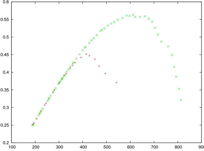
Figures 4.3 and 4.4 show the precision with respect to the recall curves for different Levenshtein threshold. The blue curves are for a Levenshtein threshold of 0.3, the green ones for 0.2 and the red ones for 0.1 . All curves for both window lengths exhibit stable precision for low recall, then a slight decrease for higher recall, then a steady decline in precision for recall value with precision lower than 0.8. This suggests that in need of a high-precision tool, it is still possible to achieve good recall. For example, requiring a precision of 0.9 for a Levenshtein query of 0.1 can still give recall higher than 0.8 using window length 2. These
0.1 0.2 0.3 0.4 0.5 0.6 0.7 0.8 0.9 1 0.1 0.2 0.3 0.4 0.5 0.6 0.7 0.8 0.9
Figure 4.3 Precision with respect to recall for Tomcat and a window length of 1. Radii value on y-axis is relative. Blue curve is for Levenshtein 0.3, green curve, 0.2, and red curve 0.1
0.2 0.3 0.4 0.5 0.6 0.7 0.8 0.9 1 0.1 0.2 0.3 0.4 0.5 0.6 0.7 0.8 0.9
Figure 4.4 Precision with respect to recall for Tomcat and a window length of 2. Radii value on y-axis is relative. Blue curve is for Levenshtein 0.3, green curve, 0.2, and red curve 0.1
0.55 0.6 0.65 0.7 0.75 180 200 220 240 260 280 300 320
Figure 4.5 F-Value with respect to the total number of accepted clones for Tomcat with a Levenshtein threshold of 0.1. Red curve is for window length 1, green curve is for window length 2
The overall accuracy of the tool is depicted in figures 4.5, 4.6, and 4.7. These figures show the number of reported accepted pairs with respect to their corresponding F-Value. The red curve in each figure is the curve for a window length of 1 and the green one is for a window length of 2. Each figure shows the behavior for a different Levenshtein threshold. All curves exhibit a maximum before they all steadily decline. Figure 4.5 has the green curve decline a little bit farther after the peak value than the others. This might be a side effect of the window length at small Levenshtein threshold.
Programs were executed until a computed F-value was suspected to be maximum. This is why curves do not have points for every radii and some curves have more points than others. It is worth noting that on both absolute and relative radii, windows of length 2 induce a slower growth rate on the F-value. This leads to longer curves for this length. Tables 4.2 and
0.3 0.35 0.4 0.45 0.5 0.55 0.6 0.65 0.7 0.75 150 200 250 300 350 400 450
Figure 4.6 F-Value with respect to the total number of accepted clones for Tomcat with a Levenshtein threshold of 0.2. Red curve is for window length 1, green curve is for window length 2
0.2 0.25 0.3 0.35 0.4 0.45 0.5 0.55 0.6 100 200 300 400 500 600 700 800 900
Figure 4.7 F-Value with respect to the total number of accepted clones for Tomcat with a Levenshtein threshold of 0.3. Red curve is for window length 1, green curve is for window length 2
4.3 show the triplet of optimal values under different configurations. Each row represents a different Levenshtein threshold and each column has values for different window lengths. The triplets’ values are in the form (radii,f-value,number of clones). From these tables, numerous observations can be drawn. First, for Levenshtein distance greater than 0.0, the number of clones for the optimal triplet is always higher using the relative radius instead of the absolute one. Second, except for the relative radius with Levenshtein threshold 0.1, a window length of 2 gives better results. Third and last, the total number of found clones increases with the Levenshtein threshold indicating the method effectively finds clones with higher Levenshtein distance. Table 4.4 summarizes the best achievable F-Value for the different parameters. Explicit value of the precision and recall for each case is given.
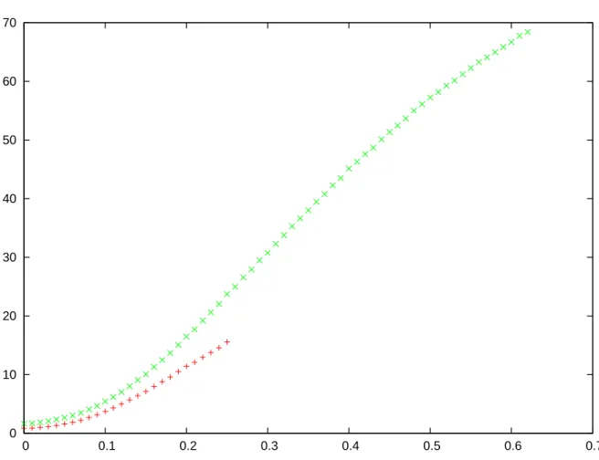
Figure 4.8 displays the variation of execution time with respect to the Manhattan distance range-query radius. The red curve is associated with a window length of 1 and the green one a window length of 2. The execution time increases monotonically as the radius increases. Execution time is also greater for a greater window length.
4.6 Discussion
Results support the possibility of achieving a good approximation of the Levenshtein dis-tance using tokens frequency vectors and the Manhattan disdis-tance. Indeed, for a Levenshtein threshold of 0.1 an F-value close to 0.88 is achieved with a very high precision. It is worth noting that at equal precision, the algorithm running does find more clones for threshold 0.2 than for threshold 0.1. Thus, if one is ready to accept a lower recall, the technique still finds clones within the region between 0.1 and 0.2 with high precision and hence could gives interesting candidates to analyze. The same observation can be applied to the 0.3 threshold. Overall, the technique has a higher precision than recall. This can be acceptable for a clone detection tool, but not as an oracle producer. However, for quick oracle production at low Levenshtein thresholds, the technique provides a reliable approximation at a fraction of the
Table 4.2 Tomcat optimal F-value for fixed Levenshtein distance and window length. Values in table are formatted as (radius,F-value,clones number). Radii are absolute values.
Window Length Levenshtein 1 2 0.0 (0.0,0.992,188 ) (0.0,0.997,188) 0.1 (8.0,0.844,267) (14.0,0.851,276) 0.2 (11.0,0.655,302) (25.0,0.685,345) 0.3 (15,0.397,399) (37.0, 0.524, 573)
0 10 20 30 40 50 60 70 0 0.1 0.2 0.3 0.4 0.5 0.6 0.7
Figure 4.8 Total execution time with respect to query radius in Tomcat. Red curve is for window length 1, green curve is for window length 2
Table 4.3 Tomcat optimal F-value for fixed Levenshtein distance and window length. Values in table are formatted as (radius,F-value,clones number). Radii are relative values.
Window Length
0.0 (0.0,0.992,188 ) (0.0,0.997,188) 0.1 (0.11,0.879,289) (0.16,0.873,286) 0.2 (0.17,0.699,342) (0.33,0.729,373) 0.3 (0.2,0.452,415) (0.48,0.563, 612)
Table 4.4 Tomcat precision and recall values for best achievable F-value Levenshtein F-Value Precision Recall
0.0 0.997 0.997 1.0
0.1 0.879 0.963 0.810
0.2 0.729 0.888 0.619
0.3 0.563 0.722 0.462
time cost.
Regarding execution time, in every configuration it increases along the increase of the absolute or relative radii. This is explained by the nature of the metric tree: as the radius increases, less of the tree can be pruned at each step resulting in more comparisons executed for each range-query, the worst-case being the all-pairs comparison. However, even with high radii, the execution time is still under a minute which is more than 50 times faster than computing the exact Levenshtein set (also using a metric tree) as shown in table 4.5. Results accuracy is at worst half the target set. This suggests that the accuracy trade-off with the enhanced speed is appealing even in more extreme cases.
Of course, the Levenshtein significance thresholds are not universal. The choice of 0.3 as
Table 4.5 Execution time of the Levenshtein oracle compared to the configuration for best results with Manhattan
Levenshtein Levenshtein (s.) Manhattan (s.)
0.0 202 1.00
0.1 1662 4.35
0.2 2984 35.30
be inserted in the tree as well as additional range-queries be performed without the need to rebuild it as can additional range-queries. Deletion requires rebuilding the entire sub-tree rooted at the deletion site. However, as shown by the execution time, building the tree is computationally inexpensive and deletion of some fragments shouldn’t hinder performances. Being incremental makes the new algorithm well-suited for clone evolution analysis.
There are some threats to validity. Results are only preliminary since they come from one system only. Therefore, no definitive statistical properties may be inferred. However, the exposed perspective opens up a whole new way to develop clone detection tools.
4.7 Conclusion
A new clone detection technique based on metric trees and the Manhattan distance has been presented. Experimental evidences show the technique to be closely related to the Levenshtein distance for small differences. Regarding the three presented research questions, the results gave interesting positive answer. It is indeed possible to give low-distortion answers to Levenshtein binary queries and the window length can improve the results overall quality. The expected limit where the technique stops emulating Levenshtein accurately seem to be between 0.1 and 0.2 .
Only preliminary results were presented, but they encourage to pursue further experiments using this technique. Some of these could include an assessment of window lengths higher than 2 as well as significance cutoff value higher than 100. Experimental evidences of the rationale supporting Manhattan distance being better than the other metrics of the li family
could also be gathered. Software clone evolution analysis as well as quick oracling are also some of the tool applications that could be investigated.
Acknowledgments
This research has been funded by the Natural Sciences and Engineering Research Council of Canada (NSERC) under the Discovery Grants Program and the Fonds Quebecois Nature et Technologie (FQRNT).
CHAPTER 5
ERRATA AND COMMENTS ON PAPER 1
At the time the paper in chapter 4 was published, a small mistake in an equation was missed by the author and the reviewers. Incidently, the same mistake was repeated in chapter 12, 4 months later and wasn’t caught again at that time. In fact, it took nearly four years before the small incoherence in the equation was finally found. Although the correction in the model is not expected to affect any of the experimental results (because it does not affect the approximation at all), it is still in order to present the errata in this thesis.
The equation:
t!
(t− l)! (5.1)
where t is the total number of token types and l the size of the window was written under the hypothesis that every token type is unique in a tuple of length l, or l-gram. While this is true for l = 1, and mostly true for l = 2, it is not strictly correct and there exists some infrequent sequences of tokens of small lengths that have duplicated token types. This becomes more visible even more true as l grows. The proper number of all different l-gram is:
tl (5.2)
which, for t = 200 is 200, 40,000, and 8,000,000 for l = 1, 2, 3 respectively. Since no part of the experiment relied on this result, it does not affect the general conclusions. However, it would be correct to note that the proportion between the observed number of different l-grams and the maximum possible number is actually smaller than what is reported and observed in the paper. Thus, in practice, the result is slightly better than what is interpreted in the original paper. Of course, a clever reader has probably already noticed that in all cases, it is impossible for the number of different l-gram to be larger than the size of the analyzed system, as it would imply that the system has more l-grams than the total number of tokens it contains, which is a paradox.
Incidently, the figures showing the examples of n-grams actually contain a contradiction with the original equation, because the figure contains an l-gram with a duplicated token. The figure can stay as it is, as the mistake was indeed in the equation. Also note that in the text, the equation is referred to as ”exponential”, while the actual equation shown is of
of false-positives will strongly affect the future F-values, making it highly unlikely that, after the sharp decline following the observed maximum, the F-values will be greater than our suspected maximum F-values.
The paper uses some basic properties of square roots to prove equation 4.10. Precisely, the inequality
√x
1+√x2 ≥
√
x1+ x2
holds because elevating both members to their square gives
x1+ 2√x1√x2 + x2 ≥ x1+ x2
and the left member is clearly greater than the right member, with equality holding if x1
and x2 are equal to 0. By induction, it can be proven that this holds for an arbitrary number
CHAPTER 6
PAPER 2: ABOUT METRICS FOR CLONE DETECTION
6.1 Introduction
Clone detectors rely on the concept of similarity and distance measures to identify cloned fragments. The choice of a specific distance function in a clone detector is arbitrary up to some extent. However, with a deeper knowledge of similarity measures, we can condition this choice to have some properties that can help improve scalability and quality of tools. This paper presents some interesting results, insights and questions about similarity and distance measures, including a somehow counter-intuitive result on the cosine distance.
For a comprehensive survey of many distances and metrics, the reader is invited to read [106].
This paper covers the following topics:
• A link between the Jaccard measure on sets and the Manhattan distance in euclidean space
• Limitations of the cosine distance on normalized vectors and approaches to overcome them
• Unanswered questions on some similarity detection techniques As a convention in this paper, we set Rn
+= [0,∞)n.
6.2 An Equivalence of the Jaccard Metric and the Manhattan Distance
Sometimes it is useful to link two known metrics to get a desired behavior or a better un-derstanding of one of the two. In our case, we link the Jaccard metric on sets with the Manhattan distance on the space Rn
+. Our equivalence holds for arbitrary sets, but different
representations in the space Rn
+ may be possible, which leads to different applications. We
δ(U, V ) = 1−|UT V | |US V | =
|US V | − |U T V | |US V |
which is known to satisfy all the metric axioms (see section 3 for a brief recall). The Manhattan distance, noted l1, on two vectors1 u, v from Rn+ is:
l1(u, v) = n
X
i=1
|ui − vi|
Now, lets associate a unique integer 1 ≤ i ≤ |US V | to every element µ in U and V . Now, choose n =|US V | and take u, v ∈ Rn
+ such as ui = 1 ↔ µi ∈ U otherwise ui = 0, and
vi = 1↔ µi ∈ V otherwise vi = 0. From this, we draw:
|U[V| = n X i=1 max(ui, vi) |U\V| = n X i=1 min(ui, vi)
The min and max terms in the preceding equations are only equal if ui = vi, otherwise
one of the two is ui and the other is vi and because |ui− vi| = |vi− ui| we must have:
|U[V| − |U\V| = | n X i=1 max(ui, vi)− n X i=1 min(ui, vi)| = n X i=1 |ui− vi|
1Actually, to define the Manhattan distance , we do not need the full power of a vector space but only
requires the n-tuples in Rn
+. However, it is now a custom to name everything in R n
+ a vector and we shall