Adjustment costs and dynamic factor demands : investment and employment under uncertainty

ADJUSTMENT COSTS AND DYNAMIC FACTOR DEMANDS:

INVESTMENT AND EMPLOYMENT UNDER UNCERTAINTY

by

GIUSEPPE BERTOLA

Laurea in Economia e Commercio,

"-Universita di Torino (1983)

Submitted to the Department of Economics in Partial Fulfillment of the Requirements

of the Degree of Doctor of Philosophy at the

Massachusetts Institute of Technology June 1988

@ Giuseppe Bertola, 1988

The author hereby grants to MIT permission to reproduce and to distribute copies of this thesis document in whole or in part.

Signature of Author Certified by

Accepted

by

,

' Department of Economics April, 1988 Rudiger Dornbusch Professor of Economics

Professor Peter Temin, Chairman Departmental Graduate Committee Department of Economics

ADJUSTMENT COSTS AND DYNAMIC FACTOR DEMANDS: INVESTMENT AND EMPLOYMENT UNDER UNCERTAINTY

by

GIUSEPPE BERTOLA

Submitted to the Department of Economics on April 28, 1988 in partial fulfillment of the requirements

of the Degree of Doctor of Philosophy. ABSTRACT

Chapter 1 studies solution techniques for problems of dynamic control under uncertainty with linear costs of control. Necessary conditions for optimality of control policies are derived from a feasible perturbation argument, and i t is shown that under

restrictive conditions the optimal policy can be based on current events only.

A

solution is explicitly derived under the assumption of constant-elasticity functional forms and of uncertainty

described by geometric Brownian motion processes. Under these assumption, an alternative approach to the solution is proposed, based on optimal stopping arguments: using well-known financial tAchniques, the solution can be found via valuation of options to exercise control at the margin.

Chapter 2 applies the control technique to the problem of irreversible capital accumulation. Under the realistic assumption that capital equipment has no value unless used in production, the optimal investment rule is derived in closed form. It is found that the degree of uncertainty facing the firm is an important determinant of the irreversible investment decision: the more uncertain are future business conditions and the more variable is the purchase price of capital, the more cautious firme should be in their investment decisions. The dynamics of the firm's value and the ergodic distribution of several observable variables are derived, and a preliminary discussion is offered of the results' implications for the empirical study of investment.

Chapter 3 studies the effect on labor demand of European severance pay legislation. The form of firms' employment policies is derived using the techniques developes in Chapter 1; firms are more reluctant to hire in the presence of firing costs, but are more reluctant to fire as well. It is found that employment is, on

average, higher when firing costs are large. The parameters of stochastic processes taken as exogenous by firms are shown to affect the employment policy in intuitive ways, and the European employment experience of the last fifteen years is interpreted under the assumption that a regime switch in the stochastic

environment of European firms occurred after the first oil shock. Thesis Supervisor: Rudiger Dornbusch

ACKNOWLEDGMENTS

In these four years at MIT I have learned a lot about

economics, about myself and about life. I am very grateful to my primary advisors: Rudiger Dornbusch saw me through the confusing initial attempts at original research, and during the past two years gave me much needed support and encouragement, as well as always insightful advice and sense of direction; Olivier Blanchard was always available and interested at what I did: he helped me a great deal to focus on substance and intuition, while his interest in the technical aspects of my work spurred major advances. I had much more interaction than is usually the case with the third reader of this thesis, Robert Pindyck; his work inspired most of what I have done, and he was always helpful and available for illuminating discussions.

I was fortunate to be Daniel McFadden's teaching assistant for two semesters; from him I learned most of what formal rigor I have. I consider a privilege to have been able to work a l i t t l e with Franco Modigliani, whom I thank for his warm interest in my progress and for always insightful conversations.

Countless other individuals have contributed to the

development of this thesis, both at MIT and at the institutions I visited while looking for a job. But the special debt lowe to my classmates and friends goes beyond i t . Ricardo Caballero was an essential part of my life at MIT, both at wOLk and at leisure. Anil Kashyap and Takeo Hoshi were wonderful officernates, generous with their time, entertaining and wise. I enjoyed discussing with Samuel Bentolila our joint work (which became the third chapter of this thesis) and the meaning of i t all. I am sure we'll all remain in touch with each other and with the other friends we made at

MIT.

Financial support for part of my years at MIT was provided by Istituto Bancario San Paolo di Torino and by Fondazione Luigi

Einaudi di Torino, to whom I am

most grateful.

lowe the greatest debt to Clara, my wife. She makes me a much better person and helps me in so many ways; without her, i t would have been impossible to go through all this. Thanks.

INTRODUCTION

This Thesis studies the optimal dynamic factor demand policies of firms subject to exogenous uncertainty, under the assumption that changes in the use of factors of production incur first-order adjustment costs: the combination of uncertainty and first-order costs of adjustment is on the one hand quite

realistic, and on the other has far-reaching implications for the study of many issues in dynamic economics.

If adjustment costs for the use of factors of production did not exist, the firm's dynamic problem would be uninteresting: all factors would continuously be adjusted so that their marginal contribution to profits would at all times be equal to their rental cost. In reality, of course, the use of factors of

production cannot be costlessly adjusted: machinery and buildings have to be installed and uninstalled, workers have to be trained, and severance payments often have to be paid to dismissed workers; second-hand capital equipment has much lower value than new

capital equipment, and is often so specialized that i t can only be sold to other firms faced by the same exogenous uncertainty. In such a situation, capital has value only if used in production, and capital accumulation is irreversible.

Realistic adjustment costs are nonnegligible even for small adjustments in factors' use; the assumption that they are in fact linear does less violence to reality than the more usual (and more easily tractable) assumption of quadratic adjustment costs.

Linearity of adjustment costs enhances the importance of uncertainty in the firm's problem. Since adjustment entails first-order costs, the firm has to be careful in exercising control over the amount of factors of production i t uses. If an exogenous shock is immediately followed by one of opposite sign, the firm will congratulate itself if i t has not adjusted to the first shock, and will regret the previous decision if it has; conversely, if subsequent shocks have the same sign as the first one, the firm will regret not having adjusted right away. Every adjustment decision must then balance these possibilities, and has to take explicit account of risk. The dynamics produced by linear ~djustment costs are very different from those produced by convex ones. Convex costs of adjustment make i t optimal to adjust only partially to any shock; with linearity, adjustment is complete if i t occurs, but may not occur at all.

Chapter 1 illustrates a set of new techniques that make i t possible to solve fairly complicated and realistic models of tnis type, and discuss their relationship to earlier economic and

financial literature and to abstract optimal control models in the mathematical and engineering literature.

The main assumptions needed to obtain the solution are that exogenous uncertainty be described in continuous time by a process wi.th independent increments and continuous sample paths, and that all functions relating exogenous and endogenous variables have constant-elasticity form. The assumption of independent increments

least, nonstationarity of the stochastic environment of economic agents can be defended on theoretical grounds <uncertainty about the future should realistically increase with the forecast

horizon) and, on empirical grounds, cannot be refuted

by

the limited time-series data available: tests on most economic data fail to reject nonstationarity of the underlying stochastic processes. The assumption of constant ela~ticity (loglinear)

functional forms is consistent with much empirical literature, and allows construction of fairly complicated models of the firm:

problems with multiple state variables can be reduced to equivalent problems with only one state variable.

Chapter 1 also shows how optimal risk taking techniques (option valuation, optimal stopping) can be used to solve

stochastic control problems under first-order adjustment costs. As noted above, every adjustment entails some risk of regret

if

there is ongoing uncertainty, and optimal stopping techniques indicate how such risky decisions should be taken.

The following two Chapters apply the control technique to economically interesting problems.

Chapter 2 studies the dynamics of irreversible capital accumulationr and the implications of irreversibility for

empirical studies of investment: the assumption that the scrap value of capital be negligible is certainly realistic at the macroeconomic level, since production facilities have no direct

consumption

value; and

is

a very close approximation for an individual firm's problem, since capital equipment is usually

specific to a firm's needs and has little (if any) resale value. The investment rule has a clossd form under the assumption that the cost of adjusting capital use downward be prohibitive, and has intuitive comparative statics properties: firms will be more

reluctant to invest if their environment is very uncertain. The implications of optimal irreversible investment decisions for observable quantities are also derived, and i t is found (perhaps surprisingly) that higher uncertainty implies that on average more capital will ex-post be used

if

uncertainty is larger and

investment is irreversible. Firms are more reluctant to invest in such a situation, but the impossibility of decumulating capital builds a ratchet in the accumulation process and increases the long-run capital intensity of production.

Chapter 2 then discusses the implications of investment irreversibility for the behavior of observable variables such as the value of the firm, investment and Tobin's Q: the dynamics of all variables are non-standard, and exogenous shocks can

potentially have very long-lasting consequences. The results of the Chapter are arguably consistent with the empirical evidence based OIl more standard dynamic and pseudo-dynamic models of

investment. Dynamic models based on convex costs of adjustment are mispecified if investment is irreversible in reality, and their poor empirical performance is therefore not surprising, but i t is

possible to interpreted their results under the assumption of

investment irreversibility. Quasi-static models of investment, based on the asssumption of equality (on average) of capital's marginal profitability to its user cost, are also mispecified

if

capital accumulation is in fact irreversible: and irreversibility can help explain recent empirical results in this strand of

literature.

Chapter 3 (joint work with Samuel Bentolila) applies the optimization model of Chapter 1 to dynamic labor demand in the presence of hiring, and especially firing, costs. The European unemployment experience has often been partly blamed on

restrictive severance pay legislation, which appears to explain well some features of the dismal employment-creation record of most European countries. A formal model shows that firms will exercise more caution in their employment policies

if

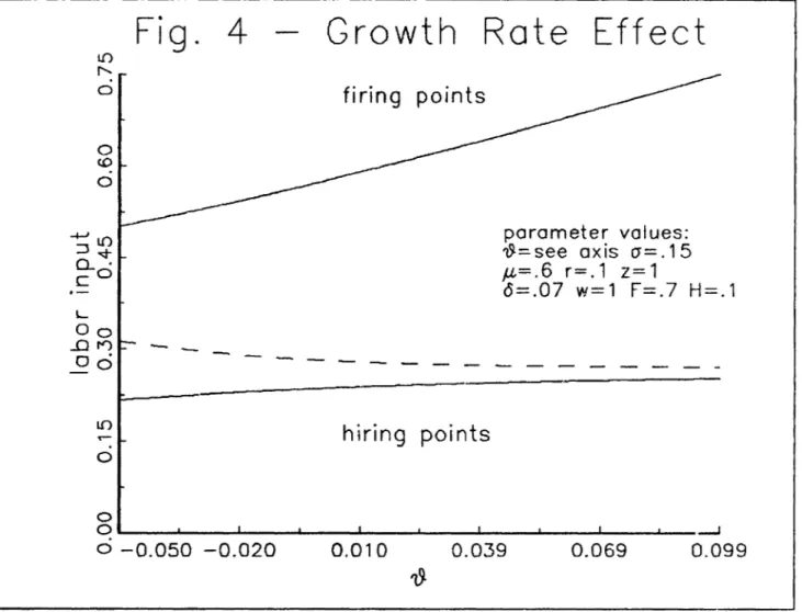
labor-force adjustment costs are large and the environment is highly

uncertain: the characteristics of the firm's employment policies are also related to other parameters, notably the attrition rate of the employed labor force and the growth rate of desired

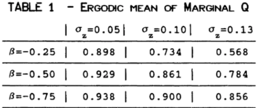
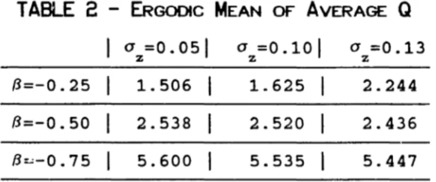
production. The implications of high firing costs for observed employment are also derived: i t is found that the size of firing costs scarcely affects the average level of employment in the long run (and, via the

same

ratchet effect found for irreversible

capital accumulation, larger firing costs increase average

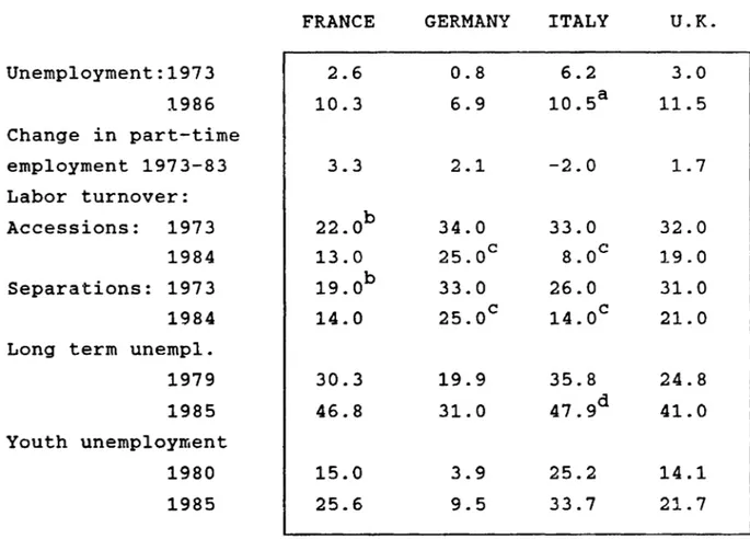
employment): but large firing costs have clear dynamic effects, inducing sluggish adjustment of em~loyment to exogenous events. The implications of the model are quantitatively evaluated with r9alistic parameters valu9s for the four large European economies: the change in firms' stochastic environment that followed the

first oil shock, and the presence of high firing costs, are found to be by and large consistent with the observed behavior of

e~ployrnent in those economies, characterized by very little hiring and firing, but large reductions in employment via labor

CHAPTER 1

This Chapter discusses the solution of a class of discounted dynamic control problems, distinguished by the fact that the cost of adjusting endogenous state variables is linear in their

displacement - i.e., the marginal cost of adjustment does not depend on the speed at which adjustment occurs. Problems of this type have been studied in the Operation Research literature;

economic applications to the theory of the firm could include the study of inventory processes, pricing in the presence of menu costs, irreversible investment decisions, and dynamic labor demand. Two such applications are considered in the following Chapters, and the set of techniques proposed in this Chapters should prove useful in future research as well.

The techniques presented below are not totally new, although their application to economically interesting functional forms is. The treatment privileges economic intuition over abstract

technical rigor: the thought experiments (feasible perturbations)

underlying

optimality conditions are described in economic terms, and the equivalence among the different approaches should

eventually

become clear to economically minded readers.

Section 1 presents the general form of the problem under

study: Section

2 proves necessity of an economically intuitive first order condition for optimality of a control policy, based on a feasible perturbation argument. Section 3 proves that the

problem under study can sometimes yield "myopic" policy rules, and refers the reader to previous work by Arrow[1968] and

allow explicit solution of the problem under uncertainty, and derives the solution making use of the necessary conditions

discussed in Section 2. Section 5 proposes an alternative approach to the same problem, based on optimal stopping rather than on the feasible perturbation argument, and uses this result to prove

existence of the solution. Section 6 discusses the characteristics of the solution and reviews related Operations Research literature on similar control problems.

1 - Statement of the problem

Consider the optimization problem of a firm (or some more general economic entity, for example Robinson Crusoe or the social planner whose optimal plan is mimicked by a competitive market) that tries to maximize a time-separable objective function. The discount factor is constant and equal to r, but instantaneous payoffs depend on exogenous factors W

t (the state of the affairs),

whose probability law the firm knows and takes as given, and on endogenous state variables K

t which the firm can manipulate. For simplicity, K

t is assumed to be a scalar. To obtain an interesting problem, we assume that manipulating K

t is costly, and we ask what is the firm's optimal adjustment policy.

In order to state the firm's problem formally, some terms are used whose (rough) definition follows: a a-field is a partition of

the states of nature ~, which are eleJ,ents of the sample space 0; statements that are made "almost surely" are true in all states of the world ~, except that they can be false for a set of ~s (an event) which has zero probability measure. If there is no memory

loss, observation over time of a stochastic process (a function of time and of the state of nature ~) generates a finer and finer sequence of a-fields, i.e. provides ever more detailed information about the true state of the world; a probability law assigns

probability measure to all sets (events) of the partition; and a random variable X is said to be Uadapted" to a a-field if

observation of XiS realization does not provide information further to that provided by the a-field (jf the a-field is

generated by a stochastic process, the adapted random variable X is "non-anticipat.ory" wi th respect to that stochastic process).

PROBLEM Given:

- the probability law P for exogenous forcing factors

(WT;OSTsool, and the sequence of a-fields r

T generated by {WS;SST}; W is a possibly vector-valued stochastic process, i.e. a function

+

n

W(~/T) :00~ ~ that maps every state of nature in w into a

complete sample path for the exogenous variables; we assume that sample paths are right-continuous.

- the functional form of instantaneous payoffs n{Kt,W

t );

- a given instantaneous discount rate r;

- _{the adjustment cost f[dXT,W T) for each unit displacement of} the endogenous state variable; f(.,.) is assumed to have the

following form: P(W T)

,

if x

) 0 [1.1]

_f(X,W

T]

=

0

if

x = 0 p(W T )

,

if x

<

a

- the spontaneous dynamics of the endogenous state variable,

given

by

[1.2] dK_t

=

-OKtdt + X

t for all t

where 6 is an exponential depreciation rate, assumed constant for simplicity;

*

~olve for the value function V and the associated optimal feedback control process {K

T : KT adapted to 7T , t~T~T), defined by

[1.3]

where

is the value function, and the conditional (on the information available at time t) expectation, Et{ ..

}=J ..

dP(~;7t)'

is taken over the joint probability distribution of exogenous variables

{W

t }

and endogenous variables {K

t }.

Some remarks on the

characteristics

of the

problem

considered

are in order. Since the problem

in

described in continuous time, the

firm can

continuously monitor

the

state

of

affairs

and

act accordingly; as i t is often the case, this turns out to simplify the

solution. Note

however that the degenerate stochastic process

(calendar time)

XT=T

a.s. could well

be

one of

the

elements of W,

and

the adjustment

cost

function could then be specified so as to

prevent

adjustment at non-integer values of T, for example, or on

Sunday.

larger displacements of K incur constant marginal adjustment costs; ttlis produces solutions with "bang-bang" character: if adjustment is undertaken, the speed of adjustment can be

infinitely large, so that the paths of the endogenous variable K fail to be differentiable functions of time (K "can jump"). The firm need not continuously adjust the factors that are costly to move, and can instantaneously displace them by a finite amount when i t does act. Since X

T can fail to be differentiable, the second integral in [1.3] is to be interpreted as a Stiltjes

integral, with integrating function dXT=XT+-X_T_- If the adjustment costs were strictly convex, then the sample paths of {X,) would be differentiable, i.e. dXT=xTdT _{where x, is the rate of control per} unit time.

Note from the form of the first integral above that the instantaneous payoff n(.,.) is instead restricted to be a flow: apart from discounti~g, additions to total revenue are n(Kt,Wt)dt in a small time interval dt. In other words, the problem is

restricted by the assumption that total undiscounted revenues TI=

Jdll

can be written as In<t}dt, or that the cumulation of revenues

is

differentiable with respect to time. Nondifferentiability of the total revenue function

n

would realistically arise

if

the firm only sold its product and/or paid variable costs at distinct, and possibly random, times. This is ruled out in [1.3] for simplicity.

Note that, for now, i t is assumed that the problem in [1] is well defined, i.e. that the integrals and the expectations exist. This needs to be verified for individual applications: further

restrictions will be specified in what follows as necessary.

2 - Characterization of the optimal path

It is possible to characterize the optimal path to some extent (if i t exists) without actually solving the problem [2] -in fact, without finding the value function.

A further assumption is necessary:

Assumption The instantaneous payoff function is twice

differentiable, increasing and strictly concave in the endogenous state variables:

for all t, almost surely;

a

K

t 2

a

n(Kt,W_t )

<

0 , for all t, almost surely;

a

K 2

t

Under these conditions, the following is true: Proposition 1 (Feasible perturbation)

If the firm adopts the optimal control rule, then whenever control is

taking

place the

following

is true (almost surely):

[2.1]

And when no control is taking place, i t must almost surely be the case that

[2.2]

e-(r+O ) (T-t) on(KT'W)T dT}

OK T

necessary for optimality of the firm's policy.

PROOF: By assumption, the firm is following the optimal dynamic

*

program: let {K

T ; O~T~TI be the stochastic process for the

endogenous variables corresponding to the optimal feedback rule.

"'"

We now prove that [2.1,2.2] must almost surely be satisfied by {K_T

: O~TSOOJ, or else the value function would not be attaining the maximum. Let A be a subset of 0, with p(A»O, such that neither [2.1] nor [2.2] are satisfied at some T<OO

if

~A; note that AEY

T, i.e. i t is known at time T whether or not the true state of the world is in A ("A occurs"), since all expressions in [2.1] and

[2.2] are observable at T. It is then legitimate to perturb the

*

original investment policy (dX

t } by a small amount A at time T if A occurs, without otherwise m~difying the feedback rule (so that the amount of control for the endogenous variables is the original one for every time except

T

and every state of the world except

*

~

all ~A: dXT=dXT+A if A occurs, and dXT=dX_T almost surely for T-T. Note that the new policy is legitimate in that i t is s t i l l adapted to

r

t , i.e. depends on an event that is known when the

perturbation occurs). By integrating equation [1.2] above, if (K ;OSTSOO) are the endogenous variable paths for the perturbed

T

*

policy and (KTiOSTSOOJ are the paths corresponding to the optimal policy, the perturbed policy under consideration are such that for

*

OSTsT K =K almost surely, and for TSTSOO

T T

,.

*

occurs, KT=K_T otherwise.

As long as all integrals and expectations are well defined, we can exploit their linearity and additivity properties to write, for any tST,

-

*

[2.3] V(Kt,W t ) -

v

(Kt,Wt ) = T

{J

-r(T-t) ( ] }

=

E

_t

e

In(K~

_{,wT>-n(KT,wT> dT}

+ t <D

Je

-r<T-t)J

-r(T-T) [ -0 (T-T) ]

=

e

U(K:

_..

+

Ae

,W >-niK*,w > dT

_{T T T} A T

>

Je-r(T-t) [J

A T -r(T-T} e

=Je-r(T-t) [J{J

A A T -r(T-T) e

The inequality above follows from the assumed strict

concavity of n(.,.) in its first argument, and the last equality uses 't£7

T for tST (the law of iterated expectations).

It is now possible to show that A can be chosen to obtain

*

V(Kt,W_t ) ) V (Kt,W

t ) if the probability is not zero that neither

[2.1] nor [2.2] will be true at some finite time.

*

Suppose first that dXT-O but,

if

A occurs, then

[2.1'] -(r+o)

(T-t)

on(K

W) }

e " T dT

oK

_T

= -~ 74 0

contradicting [2.1]; note that, since by assumption i t is known at T that the true state of the world is in A, P(W;;T)=O for ~€{Q\A}

(the complement of A) and therefore

-(r+

o)

(T-t) on(K ,W ) e T T 8K T

=J J

Q

T

=J J

A T - (r+o) (T-t)

on

(K , W ) e T T dT dp(~;'T)

oK

_'T

.

,

Choose a A with the same sign as ~ and smaller in absolute

*

value than dX

T, so that (recalling the definition of f(.,.) above) f(dX;+A,WT]=f(dX;,W

T]. This choice for A yields, after insertion of

[2.1']

into

[2.3],

[2.4] V(K_{t '}W)_{t -} V*(K_{t '}W)_{t )}

J

e-r(T-t)A

~ dp(n'·~t)

I I ~ ~ r

A

But the right hand side of [2.4] is strictly positive if A has positive probability, which contradicts the assumed optimality

*

of the feedback rule which produces {K T }.

Suppose instead that dXit=O but [2.2] fails, for example

T

{J

-(r+o) (T-t) 8n(K W) }

[2.1']

p(W

t ) -

E

t e T' T dT

=

~

< 0

t

OK

_T

Then set A<O and obtain from [2.3] the inequality

*

J

-r(T-t)

V(Kt,W

t ) - V (Kt,Wt » e A ~ dp(~;7t) >0 A

If i t is the second inequality in [2.2] to fail, then choosing a positive

A

will yield a similar inequality.

We conclude that any failure of [2.1,2.2] that occurs with positive probability implies that the firm is not following the optimal feedback rule in its control policy, in that a feasible feedback policy would yield a strictly larger value function.

[end of proof].

straightforward interpretation: whenever the firm is in fact acting, concavity of the payoff function implies that at the margin the action does not alter the value of the policy; the value of the last infinitesimal unit of K. installed or

1

uninstal1ed at the present time\is simply the expected, present discounted value of the contribution to instantaneous payoffs by

the infinitesimal unit that will 'be marginal at all future times \

i

(the shadow price of K). If the firm is not acting,_, that expected, present discounted value is (weaklr) less than the certain,

t

\

immediate cost of adjustment.

The firm should then, when de~iding about the amount of control to be applied at the present time, view the currently

marginal unit as the marginal one t~roughout the planning horizon, and take future investment decision~ as given in probability

distribution. The very fact that con~itions [2.1] and [2.2] will be satisfied at all future times then defines the optimal control policy.

This can be interpreted as an i~plication of the envelope theorem: the firm is justified in ta~ing future control as given when deciding on the amount of control to be applied today,

because any effect of today's control on future value has to occur through a modification of

future

investment decisions; ~ut

these

are assumed to be optimal, hence at the margin a small change in future control has no effect on the value function.

I t should be noted that this characterization can be obtained imposing

very

l i t t l e structure on the problem. Apart from the

concavity of the payoff function, i t is only assumed that policies are non-anticipative with respect to the exogenous variables, that all the integrals and expect~t~~ns are well-defined and therefore have the usual linearity and additivity properties. Once again, exist~nce of the value function needs to be verified for specific applications.

3 - Myopic policy rules

Recall that i t has been assumed above that the exogenous variables {WtJ have right-continuous sample paths. An additional assumption will guarantee that p(.), P(.), n(K,.) and an(K,.)/oK have right-continuous sample paths as well:

Assumption: peW),

pew)

and n(K,W) are continuously differentiable in

w.

This, together with the characterization obtained above for the optimal control rule, suffice to obtain an important result: Proposition 2 (Euler equation)a) If an optimal feedback rule exists, and dXT-O for TE[t

1

,t

2) I

t

1

<t

2 (i.e.control of the

endogenous variable takes place with probability one between t 1 and t 2) ,

then

[3.1]

on(K ,W ) T T

oK

_T

PROOF: Since control occurs continuously in [ t

1,t2) , we have from

-(r+5) Cr-t) Q1l(K ,W )

e T T

8K

T

almost surely for tE _{[ t} 1, t2>

For a fixed w, consider the path-by-path differential of the two sides of equation [3.2] with respect to t (the differential is well defined since W - and therefore K - have right-continuous sample paths) to obtain:

[3 .3] df (dX (c.> , t) , W(c.> , t) ]

₌

8n(K(Q,t) ,W(~,t» dt aK(CA>,~-)

- (r+0) (T - t ) ]

(r+5) e Qn(K(c.>,T),W(c.>,T» dT dt

OK((,),T)

which is true for all tE _{[ t}

1, t2) and all ~E{Q\AJ, where A is any

subset of 0 such that p(A)=O.

Now integrate both sides of [3.3] over 0 with respect to P(~:7t)' noting that any ~ such for which [3.3] is not satisfied belongs to sets that receive zero weight in the integration, and that K

t and Wt are known at time t so that integration over states af nature of the first term on the right-hand side of [3.3]

returns its actual value:

+ (r+6) e- ( r +0) (T - t )

a

11(KT'W)T dT}

oK

_T

from which the assertion follows noting from equation [3.2] that

the last term is e ~ (r+~~~Xt,Wt}~.~---~ [end of proof]

Proposition 2 states the conditions necessary for the firm to temporarily base its control policy only on current events,

without looking forward and with no need to take the endogenous variable's process into account. Note that the proof does not go through as soon as there is any probability that i t will be

optimal to abstain from control in the next instant. In

particular, of course, there is no presumption that a condition like [3.1] should hold when the firm is abstaining from control, i.e. when dX=O.

The economic interpretation of [3.1] is straightforward: if control is certainly occurring throughout [ t

1,t2) , then i t must be

distributed along that interval in such a way that [3.1] is true. Otherwise, a reallocation of control would increase the value of the firm: in other words, a version of the Euler equation would be violated.

Arrow[1967] and Nickell[1974] used the equivalent of [3.1] to characterize investment under linear adjustment costs, assuming that the exogenous variables in W follow piecewise continuous paths, about which the firm has no uncertainty: then when

investment occurs, i t occurs continuously over an interval, and consi~eration of

[3.1]

is sufficient to solve for the path of the endogenous variable K. Control (investment) will stop and resume at points in time where

[3.1']

an

(K , W )

'r T

oK

_T dT

a~d knowledge of the exogenous variables' path will suffice to construct the optimal investment policy: Arrow and Nickell provide algorithms for this purpose, and show that iI1 general investment will stop before a cyclical peak is attained and resume after the cyclical trough.

If control is certain to occur at all times, i.e. the

equations in [2.1] always hold with equality, then [3.1] is always true and the firm can follow a "myopic" policy rule, varying the endogenous factor K so as to equate its current marginal payoff to

the current value of the right-hand side of [3.1]. A sufficient

condition for this to be the case is that PCWT)=P(W_T ) for all T,

almost surely: then [2.1] and [2.2] collapse to the single equation

[3.5] , all t

In such a situation, of course, the firm does not need to solve a

truly

dynamic problem: use of K_t can be varied

called liIuser cost of capital" (see Jorgenson[1963]) if K is the

installed capital stock.

4 - A class of solvable-problems

Consider the following specialization of the general problem described in [1] and [2] above:

{Wtl={Wzt,Wptl is taken to be a two-dimensional Brownian motion process, i.e. each state of the world ~ is associated with

constant elasticity

a

two continuous sample paths wi th increments (W,."

-w ,." ,

W ' Y

-w

' Y ;

z.2 z~1 p.2 p.1 T2)T1} which are independent of fW

Z'Tl'WpT2} and have a bivariate

normal distribution given the information available at Tl:

1

[4.1] W(Kt,Zt) = 1+8

K~+8

Z t ' -1<8<0,

function of the endogenous and exogenous state variables, with [4.2] dZ_t

=

~z Ztdt + Zt U

z dW

zt '

a univariate geometric Brownian

motion process: P

t follows a geometric Brownian motion with stochastic

differential

where dW_pt is the increment of another standard Wiener process with correlation p to dW

zt;

[4.5]

P

t

=

~ Pt , ~ constant, Asl to satisfy the assumption that

ptSP_t

always.

The problem data are ~, ~ I ~ I U I 0 , P, A, 0 and r: all

z p z p

these are assumed to be constant over time.

Note that geometric Brownian motion processes are particularly convenient since their Markov state space is completely described

by

their level alone; and assuming a

constant-elasticity functional form for the instantaneous payoff

facilitates solution because constant-elasticity functions of

geometric Brownian motion follow geometric Brownian motion.

The restriction -1<8<0 makes Proposition 1 in the previous section applicable: we then seek a non-anticipative control rule that satisfies [2.1] and [2.2] at all times: i.e., the optimal control rule must specify a nonanticipating control process (X

t ) such that

[4.6]

- (r+

o)

(T-t) 13 e K_T ZT (J)

r

r -

(r+0)

(-r -

t ) {3 } [4.~] E

tLJ

e

K-r Z-r d-r

=

Pt

if dXt<O

t

With the assumptions made above,

it

is reasonable to guess that the optimal control process 'will have the following form: the

endogenous

variable

should be displaced

only

as necessary to

obtain

[4.9]

or equivalently

where the boundaries a and ~ are constants to be determined. Such

a control rule is obviously nonanticipating, since it only depends

on current values of the exogenous variables, which in turn

have continuous sample paths.

To verify that the control rule has the form [4.9], and to find the optimal control barriers ~ and

a,

i t is now necessary to compute the expectations of di~counted marginal payoff streams appearing in

[4.6]-[4.8].

The problem at hand is to find an expression for the

conditional expectation appearing in [4.6]-[4.8]; the conditional expectation will, of course, be a function of the current value of the state variables and of the parameters 0, r, a,

.e,

{tI {t , a I

p Z

a

p '

n.

Define a new variable nt

=

K~

Zt'

and define a functional expression for the conditional expectation:

(I)

[4.10] f(nt,p

t ; 0, r, {I" t . . . .

J

=

Et{I nT

e-(r+~>

(T-t>dT } t

Of course, the control rule in [4.9] has to be taken into account when computing the conditional expectation in [4.10]: the process followed by (ijt) under the control rule needs to be

determined.

Now note that when control is not enacted, i.e. dX

t is zero,

then dK_t=-6 dt, and the derivative of the payoff function with respect to K follows a geometric Brownian motion, being a constant

f3

elasticity function of geometric processes; define ~t

=

{K

t Zt; dXt=Ol, and use Ito's lemma to find its stochastic differential:

a~

a~t

1

[a2~t

[

]2

[4.11]

d~t

=

t dK

+ ----

dZ

+ -

----

dK

t

+

oK t

aZ

t 2 8K2

where ~=

-6B

+

~_z

.

If a control policy of the form [4.9] is adopted, the firm will prevent {~tJ from ever being larger than a P

t or smaller than ~ Pt=~~Pt;

the derivative of the

payoff function with respect to

K

than follows a regulated geometric Brownian motion, with moving control barriers at a P

t and l A Pt : i.e. the stochastic process

Inti

is defined by

[4.12]

n

t

=

where:

(i) {~t} is a geometric Brownian motion process, with stochastic

differential

d~t

=

~t

P

dt

+

~t _GzdWzt

and initial condition ~O: (ii) {UtI and {L

t } are increasing and continuous processes, with

L

_o

=u

₀

=1:

when ijt=ap

t

, where

a and

~

are given positive real numbers and P

t

follows a geometric Brownian motion, with stochastic differential

dPt=~pPt

dt

+

_{Pt a p dWpt}

' dWztdWpt=pazap

and initial condition PO' such that

~APO $ ~O $ aPO~

(iv) ! S i j t s a for all t~O

These

four properties uniquely identify

(Uti and

(Ltl: these two processes maintain ijt within. the moving barriers us~ng the minimum amount of control, since they only increase when i j t i t at

the frontiers of the region

el,a].

Proposition (6), page 22 in Harrison[19851 proves uniqueness formally for the case of a

regulated linear Brownian motion process, and i t is

easy

to adapt the proof to the present case of a regulated geometric Brownian motion

process:

note

that

(7

1

_t

/P

t)

is a

geometric

Brownian motion

process regulated between Al and a, implying that fln(ijt/Pt)} is a linear Brownian motion process regulated between In(A~) and In(a) I

and apply Harrison's proof of uniqueness.

It is now possible to compute the expectations of discounted marginal profitability streams appearing in equations [4.6]-[4.8], as a function of the yet to be determined control points t and a,

and of the problem

data.

First note that {UtI and (Ltl are processes of finite variation, since they never decrease: this means that

2 2

(dU_t ) =(dL_t ) =(dUtdLt)=(dUtd~t)=(dLtd~t)=O.

These relations imply that

if

we apply Ito's lemma to ~t'

which is a continuously

differentiable function

of

~t' U

t

and L

t ,

L ~ ~ d~ + _ t dL U t U t t t L L _~t dL t ~t L t dUt _ t

~t

IJ dt

+

_ _t G dW t

+

_L t

- - -

-U t

u

Z Z _U t Lt Ut Ut t

=

T1 t lJ dt + 71tC7zdWzt + 71t dL t dUt - - T1

--L t _U t t

Now

consider the conditional expectation defined in [4.10],

f(71

t ,Pt) (the dependence of the function on the time-invariant parameters r, 6, at l . . . is suppressed in what follows for typographical convenience); assume that i t is a continuously differentiable function of ~t and P

t , and apply Ito's lemma again to obtain (subscripts denote partial derivatives):

only if ~t=aPt' is used in obtaining the last equality.

Now recall the Integration

By

Parts formula found in

Harrison[1985], page 73: if fY

t } is an Ito process (i.e. the

stochastic integral IdYt is well defined) and (Xtl is a continuous

process with finite variation, then

lJ lJ

YvXv

=

YtXt + IYTdXT + IXTdYT

o

0

Apply the Integration by Parts formula to Y_v= f(nv'p_v) and

x

_v

=e-(r+5) (v-t)

, which always decreases and therefore has finite

-(r+6) (T-t) (r+O) (T-t)

variation; using dee ]

=

-(r+O)e dT, and

df(~T,PT) from [4.14], one obtains, after rearranging terms,

[4.15] _e-(r+o)vf (_{l1v '}P )_v =

v

+Ie-(r+o) (T-t) [f1(71T,PT)71T

P

+ f2(71T,PT)i}PPT+ :

f

_u

_{(71 T,PT)a:71;+}

t

1

2

f22(71T,PT)a;p~

+

f1~(71T,PT)71TPTpazap-

_{(r+O) f(71 T,PT) ] dT +}

I

f1(A~T,PT) A~PT d~:

+ I f2(71T,PT)PTO'pdWpT

t T

For the investment rule to be well defined it must be the

case that f(.,.) and its derivatives are always finite; this

and, for all v ~ t,

v

v

E_{t {}

If

1

(ijT'PT) ijTCzdWZT }

=

Et {

I f2(ijT,PT)PTCpdWpT}

=

0

t t

because the expectation of the integral of a bounded function against a Wiener process is always zero (see, for example,

Proposition 4.3.7 in Harrison[1985]: this is due to the erratic behavior of the Wiener process, whose increments after time tare completely unpredictable, by definition, on the basis of the

information available at t).

Then, let V~ and take the conditional expectation of [4.15] at t to obtain

[4.16] 0

=

e-{r+6) (T-t)

[f

₁(TJ_{T '}P)71_{T T}J.l

+

1

f 22 (ijT'PT)C;P;

+

£12(77T ' PT)77TPTpazap - (r+o)

_{f(ijT'P T) ) dT}

_{} +}

2 (J) 00 Et {

I

£1(aPT,PT ) aPT dUT

I

f 1(A..lpT'PT ) A.lPT dL T

}

-U T

L

T t t

- (r+O) (T-t)d }

T1 e T •

T '

In light of [4.16], this can be true only

if

on the one hand

for all

nand

P such that

Als(ij/p)~a ,

and, on the other hand, the

last expectation in [4.16] vanishes: this requir~s that

[4.18]

f

(ap,p)ap

=

f

(Alp,P) Alp

=

0 for all P

1 1

We conclude that, in general, the conditional expectation

f(ijt'P

t )

is defined

by

the functional equation [4.17] with

boundary conditions [4.18].

The general form of the solution to [4.17] is a linear

combination of power functions and of a linear term,

Imposing the boundary conditions [4.18] on the functional

form in [4.20] we find:

These conditions must be satisfied for all p~O, which

[4.22]

~1=1-al, ~2=1-~

[4.23]

a

0.2-1.

= ,

0

In light of [4.22], we can rewrite [4.20] as

and proceed to compute the partial derivatives of this function to find that, for [4.17] to be satisfied,

1 8

1-r+6-IJ

and at, a2 must be solutions of 2 o

[4.25]

-2 2 2 2 where 0 E a

+

a - 2po a

>

0 z p z p

The quadratic equation [4.25] has two real roots of opposite sign provided that r+6-~_p>0· let cu be the positive root and_, Q2 be the negative root:

a1 a 2 -~ (J ) 0

<

0

1

1

0 2

1+~

Note, for use below, that r

>

-~ -+ ~ (1 +-) + - implies

that -Bcu)l, as can be verified noting that -Bat is the positive

solution to the

quadratic equ3tion

[4.26] 2 o 2 1 1 0 2 1 X -

(it -

+

6 -ft - - - - ] X -

(r+

o

--'p]

= 0 z 8 p 8 2 B [4.28] A.f s

The only parameters as yet unsolved for in [4.24] are B

2 and

B

3

: but insertion of B

1

=

(r+b-p)-1 in [4.23] yields a system of

two linear equations in B

2 and B3, with solution

1 a a2"Al _ a (A.f)a2

[4.27]

B

2

=

r+o-IJ

_al

(aal

_(:\.f)a2

aa2

_(:\.f)

al]

«(Al)a! a1

1 - a ;\,-l

B₃

=

r+

o

-11 _a2

(aal

_(:\.f)a2

a

_{a2 (:\.e)a1 ]}

This completes the derivation of

(J)

8 _

{J -

(r+0) (T - t ) {3 }

f(KtZt,P

_t :

a,

l . . . ) ;

E

_t e

K

_T ZT dT

t

under the assumption that the firm adopts a control rule that obtains

13

K_t Zt P

t

using the minimum amount of

control: control dX_t is applied to K_t

only when one of

the

weak

inequalities in

[4.28] holds with

equality.

f3

control policy, W3 insert f(KtZt,P

t :

a,

l . . . ) into the necessary

conditions [4.6]-[4.8]:

[4.6'] _{f (:\4't ' p t}

a,

.e

...J

=

:\.p_t

(dXt<O

..

K~Zt

=.f:\pt) [4.8'] _{f ( upt ' Pt} a, .e

·..J

P t (dXt>O B =

..

Ktzt=aP_{t )}

Using [4.24], these conditions read

[ 4.6"] B;t-lp B (A.4' )a1p l-al+ B (A.lp )a2pl-a.2 =

1 t + 2 t t 3 t t

P

t can be eliminated from these equations; then, insertion of

the expressions found above for

B

1

, B

2

, B

3

, and some

simplification, yields:

These two equations are highly nonlinear in u and l, but can

to prove analytically the uniqueness of their solution, numerical procedures are not at all sensitive to the starting point of the iteration, suggesting that the solution is indeed unique.

Closed-form solutions can be found for special cases: if A=l then the two equations have the same form, and cannot be solved for distinct « and ~. But with ~=1 [4.6] and [4.8] are infact the same equation, implying that «=~; then

r

Off (K

t ,Zt)/8Kt ]/Pt is

constant, and simple integration on [4.6] or [4.8] shows that the solution to the optimal control problem simply equates the current marginal contribution of K to the payoffs to the current "user cost" of K, (r-~p+5)Pt' confirming that when Pt=P

t for all t the firm will continuously exercise control (see the discussion after Proposition 2 above).

If ~=O then i t is clear that dX

t is never negative ([4.8] never applies) since

[8n(K

_t

'Zt)/8K

_t ])O always for

K>O:

this is the case of irreversible accumulation of K. The firm only exercises positive control, and K only decreases via depreciation.

Given that ~O, i t is possible to find a closed-form solution for

a.

The requirement that f(.,.) be bounded imposes that B

3=O in

[4.20] above, since in the

absence of negative control i j t can

become arbitrarily close to zero; the boundary condition then provides a closed-form solution for a. The derivation of the solution proceeds along the lines discussed above, .. and is no~

reported to save space; the form of a for the case of irreversible control is reported in the next Chapter (see [R]).

The next section uses an alternative approach to the solution

of the control problem, and finds a sufficient condition for

existence of a solution (finiteness of the value function).

5 - An alternative approach to the solution:

Marginal

Option

Pricing

The dynamic program defined in [4.1] above can be decomposed

in a

sequence

of optimal stopping problems: rather than deciding

how much control should be exercised at any given time, the firm

should decide when each infinitesimal particle of K should be installed. This approach to the problem (which was first proposed

by Pindyck[1986]) uses more familiar mathematics than the approach used in the previous section, but is based on somewhat less

economically intuitive thought experiments.

When deciding about the optimal timing for installation of

the KLh marginal unit of capital, the optimal stopping problem

facing the firm is in the form considered by

McDonald

and

Siegel[1986] for

the

case of ~=O (no resale possibility) and extended by

Dixit[1987l

to the

case in

which

the

decision

can be

reverted.

The general form of the optimal stopping problem considered

by

these authors is as follows: an asset with value v can be

purchased at price P, if not purchased

yet,

or sold at price p, if

already

purchased. McDonald and Siegel

assume that both the value

of the asset v and the purchase price P are uncertain, and follow

geometric Brownian motion: but they impose that no resale be

possible, so that the exchange of the option for the asset is an irreversible decision.

They

note that the value of the asset could simply be equal to the present value, appropriately discounted, of the dividends i t will provide to its owner (but not, of course, to the holder of the option): the asset must produce dividends, or i t would never be profitable to buy i t since i t cannot be resold. Dixit, on the other hand, considers the case of reversible

decisions but restricts P and p to be both fixed (nonstochastic).

In this section the optimal stopping technique is applied to the decision to install or uninstall the currently marginal unit of K: i t will be shown that the firm's problem can be reduced to a sequence of stopping problems of the form outlined above.

Consider that at any time, given that the total installed stock of the endogenous variable is K, installation or

uninstal1ation of an additional (K~h) infinitesimal unit of capital is possible; installation will produce a stream of

marginal payoffs whose expectation is easy to compute, because

it

only depends on the exogenous probability law of Z.

Define the "dividend" provided by installed marginal units of K (its marginal contribution to the payoff) as

[5.1]

for each

K, KE[O,OO).

unit, i.e. the expectation of the stream of marginal payoffs i t

will produce. The presence of depreciation introduces some

complications: note that installation of the Kth unit at time t

· th -t 1 t k t

future tl.-me

~

by only e-O(T-t)

1ncreases

e capl. a

5 oc a

any

~

<

1

units, since

the unit steadily depreciates at rate 0; then note that the total capital stock also depreciates at rate 6, and therefore the

depreciation

rate appears

twice in the expression

for the additional payoff produced by installation of the marginal unit of the endogenous factor when the current stock is K:

[5.2]

(I) V(K,Zt) = Et{J -r(T-t) _{-0 (T - t) ( -0(T - t )}

J

13 dT} e e Ke _ZT = t (J) J -(r+O ) (T-t) ( -0 (T-t»)13 Et{ZT}dT

=

e Ke

₌

t (I) =J - (r+O) (T - t) [ -0 (T - t ) ] 13 {} (T-t) z e Ke Z e d't"

=

t t K{3 Z t = r+O-(-' -6(3)_z TIt

=

r+o-(-'

_z-013)

The firm holds the right to pay P

t and acquire, at

any

time,

the currently marginal unit

of K, and forever receive the stream of marginal payoffs whose discounted expectation is given in

[5.2],

reaardless of future control of the endogenous stock; on the other hand, the firm can always sell the marginal unit of

capital, receiving APt but giving

up

the stream of marginal

If the firm does not purchase the Kt..h unit, a "dividend" is

given up: uninstalled units do not produce,

and

payoffs are lower.

But if the right to install the Kt..h unit is exercised, the

firm gives up the option to wait and learn information about the

evolution of

rZ

t } and {PtJ: i t is often the case, of course, that

installation turns out to be a bad idea ex-post, because Zt or P

t

fall; conversely, uninstallation can turn out to have been a bad idea if Zt or APt rise. This defines an optimal stopping problem for the decision to install the currently marginal unit: the firm has to trade off the foregone dividends and the risk of acting too soon.

The value of the marginal unit available for installation at time t has, given that the already installed capital stock K

t is

depreciating at rate -8, dynamics given by Ito's lemma as

13 d(K_t Zt)

r+o-("

-0(3) z = =

purchase price of K follows the dynamics given in [4.4] above:

dP t

=

Pt~pdt

+

_{Pt 0pdWpt}

and the resale price of K follows:

dAP

t

=

APt~p

dt

+

AP

t

a dW

p pt

Therefore, the value of the marginal unit in place, its purchase cost and its resale price follow geometric Brownian motion processes; the correlation between the increments of the first process and the increments of the latter two processes is

P,

while the purchase

cost

and

the resale price have perfectly correlated increments.

Now define a marainal option valuation problem: at any given time, the firm can exercise the call option to purchase, at price P

t , a package containing the currently marginal unit of K and a put option to sell i t at price APt; alternatively, the firm can exercise the put option to sell, at price APt' the package

containing the currently marginal unit

of K

and the call

option

to

install the next unit of K.

Clearly, the value of the two options must, for given K, depend on the current values of ~t and P

t , which completely describe the state of the system; denote F(ijt'P

t ) the value of the call option, and f(ijt'P

t ) the value of the put option. Ito's lemma

gives the dynamics followed

by

the two options

when

"alive"

(not

yet exercised). The expected rate of return on any unexercised option must then, by arbitrage, be such that the their holder earns the required rate of return: here, again, the presence of depreciation introduces some complications. The required rate of return on assets is r in the problem considered in Section 5:

since the value of the firm is the expected flow of cash-flow discounted at rate r, the opportunity cost of funds for the firm

is equal to r. But unexercised options to install or uninstall units of K should instead earn a rate of return equal to

r+o:

when such options go unexercised capital depreciates at rate 0, and the index K of the currently marginal unit steadily decreases. The optimal stopping problem is defined on a "moving target": the asset that can be purchased (the marginal option) changes continuously, a~ capital depreciates.

Imposing then that unexercised options earn an expected rate of return equal to (r+6 ) , the following functional equations are obtained for the value of the two options when alive:

(r+O ) f (11,P)

=

0

1

1

[5.4] F 1(71,P)71Jl

+

F2(71,P)~pP

+ -

Fu (71,P)O:71 2

+ -

F 22 (71,P)O;p 2 -2 2 ( r+O) F (11 , P )

=

0

where subscripts denote partial derivatives.

The solution of these ordinary differential equations must

satisfy the following

boundary conditions:

F(O,P)=O for P>O, because the option that gives its holder

the right to purchase the asset with value

~/(r+o(l+~)-~~)

must be

worthless when ~=O forever and the exercise price is positive (0 is an absorbing state

for"

geometric Brownian motion process);

f(x,P)~ as x~

if

P(OO, for the symmetric reason that an option to sell an asset with very large value at a finite price must become worthless as the value approaches infinity.

In view of the parabolic form of the functional equations, we can guess the following functional form for the two options:

B 1 T/

alp(31 [5.5] F(71,P)=

with a1)O, U2<O to satisfy the boundary conditions above.

The two options will be exercised on loci in (ij,P) space that

*

*

are implicitly defined by a function ~ =g(P ) for the call option and ~*=h(P*) for the call option, and satisfy the following

conditions: *

*

* F(g(P ),P» + P

=

g(P

*

)/(r+6(1+B)-~ ) + z

*

* f(g(P ),P )

These condi tions simpJ.y impose that the exchanges of assets performed at the exercise points be "fair", i.e. that the value of options surrendered plus the exercise price be in each case equal

to the value of assets and options received.

To solve the firm's problem, we need to determine g(.) and h(.): from the definition of ~, knowledge of g(.) and h(.) will suffice to implement the optimal policy from the observation of the current values of K, Z and P.

since the value of the assets to be received in exchange for a price proportional to P is proportional to ij, i t is intuitive

(and can be formally proved in the present setting adapting the arguments of McDonald and Siegel[1986]) that the boundary loci should be homogeneous of degree 0 in ij and

P,

i.e. that for some

constants a and ~ g(p)=ap

h (P)=:\..fp

The following conditions are then obtained:

*

*

*

[5.7] F(ap ,P ) + P

=

ap

*

/(r+6(1+fl)-~ ) +

z f (uP

*

, P )

*

Additional boundary equations are needed for determination of the boundaries and of the option values: these are the so-called "smooth pasting" or "high impact" corldi tionsI which can be derived

from the fact that the exercise boundary is freely chosen by the holder of the option to maximize the option's value.

Merton[1973 , footnote 60] proves the necessity of the smooth pasting condition for a simpler problem (optimal exercise of an American call option), but his arguments are easily extended to the present setting where the exercise boundary is common to two linked option pricing problems (one an American put, one an

American call) and the exercise price is uncertain. Merton notes that exercise points are chosen to maximize the value of the

options: in the present setting,

if

extended option values

F

and f

are defined over the space of possible exercise loci, i t is true that

[5.8] F(~,P)=Max F(~,p,a,l)

a,

.e

[5.9] f(~,P)=Max f(ij,p,a,l) -a, .t.

Replace

F

and f for F and f in [5.7] and totally

and f in [5.8] and totally differentiate with respect to l, to obtain (subscripts denote partial derivatives):

*

*

*

[5.10] F (.u,p ,P ,a,.e) p

1

=

'*

*

*

*

*

*

P /(r+O (l+f3)-ft

z + f 1(ap ,P ,«,.e)P + f3 (ap ,P ,a,.e)

Now note that F.=F. and f.=f. (i=1,2) by the definitions in

~ 1 1 1

[5.8] and [5.9]; and, since a and ~ maximize f and F, necessarily

*

f.=F.=O

(j=3,4). Simplifying P and AP. out of [5.10] and [5.11],

J J

the following additional boundary equations are obtained:

It is now easy (though tedious) to insert the functional

forms in

[5.5]

and [5.6] into the differential equations [5.3] and

[5.4] and the boundary conditions [5.7], [5.8], [5.12] and [5.13]

to determine the exercise points a and ~, as well as the unknown constants B

1 and B2 and the exponents cu, a2, ~1, ~2. As in section 4, i t is found that ~l=l-CU and ~2=1-a2 necessarily, to satisfy conditions [5.12] and [5.13] for all positive prices; replacing the partial derivatives of f{.,.) and F(.,.) into the functional equations [5.3] and [5.4] determines that al)O and

U2<O

are the solutions to the same second-order equation found in Section 4; boundary conditions [5.12] and ~5.13] can be used to solve for B

1 and B2; and, finally, [5.7] and [5.8] give, after sUbstitution of these values for B

1 and B2, a pair of nonlinear equations to be solved for U and t that are exactly equivalent to

[4 . 6II ] and [4. 7 .. ] .

The marginal option pricing approach then gives the same solution to the firm's problem as the technique proposed in

Section 4, based on the necessary conditions [2.1] and [2.2]. The economic intuition behind [2.1] and [2.2] is probably more

straightforward than the thought experiment which underlies the marginal option pricing technique: the reduction of the dynamic program to a series of optimal stopping problems is awkward, especially in the presence of depreciation. But the techniques used in this section are probably more familiar to economists (at least to financial economists) than the mathematics adopted in Section 5; and extension of the model (for example to a Leontief production function as in Pindyck[1986], or to discontinuous processes for the forcing variables {W

t ) is probably easier if the marginal option pricing approach is adopted than otherwise.

It is now possible to verify existence of the optimal policy, i.e. finiteness of the value function, because an useful byproduct of the option pricing approach is the total value of the firm: this value must be the integral of the value of all infinitesimal units of K, both those installed (whose value is v as given in

13

[5.2] plus the value of the options to Gell them, f(K Zt'P

t ) ) and those that the firm may decide to install in the future (whose value of these is F(K8Z

t ,Pt) ).

The total value of the firm is then

=

(J) +

J

B₁

(x

8

Zt]CUp~-a1

dx

= =

K_t

__Zt_ [1 1+8]K

t

B

(z

J

a2_pl-U2 [

1

r+o-(~

-08) 1+8

x

+ 2 t t 1+8a2 z 0

1+1302]

K t It +

o

<D ( ] _[ 1 Itl +I3 U l] + B Z at_pl-a1 1 t t 1+f3u1

K

_t

The first two integrals in [5.14] are easily seen to be convergent as long as -1<8<0 and a2<O. Convergence of the last integral requires 1+8cu<O, or al)-1/8: this completes the study of th~ control program, since the value function (and hence the optimal policy) is shown to exist if and only

if

cu)-l/~.

Recalling [4.26], we have the following:

Proposition The control problem proposed at the beginning of Section 5 has a solution

if

and only if

1 1 a2 1+13

r ) -It_z

_{- +}

it (1 + ) +

-B p B 2 B2

This says that the value of the firm will fail to be finite unless the expected real interest rate in terms of K, r-~ , is

p

sufficiently small compared to ~ , the expected growth rate of the z

payoffs for given K. Intuitively, when the payoff function grows too

quickly

and/or the price of

K

falls too fast, control policies can be devised that produce cash flows streams whose expected

value over the infinite future fails to converge when discounted at rate r.

6 - The characteristics of the optimal control process;

Connections to the engineering

literature

In the previous sections the optimal policy for the firm's problem under linear costs of control has been found, using

techniques based on economically

intuitive thought experiments. In this section the characteristics of the control process are

discussed, and the technical literature that has studied similar

problems in the abstract is referenced.

The reader

should,

first of all, be reminded of the

characteristics of the Brownian motion process assumed above for

the

exogenous variables in the

firm's problem,

(P

t ) and {Zt}. The

Wiener

process

fW

t ),

or

standard Brownian motion, has the

following important property: W

T1

-W

TO

is distributed

independently

of

W

T2

-W

T1 for all T2)Tl)TO. This is very convenient, because

it

implies that

the

state of the system is

completely

described

by

the current value of

W

t ,

independently of past events; but if the

process has nonzero variance, this property implies that

rWtJ

has infinite variation, i.e. that Brownian motion

"fluctuates

very

fast" (which is the reason why (dW

t )2=dt, a result repeatedly used above): Brownian motion moves both up and down in any interval of time, no matter how small.

It follows that the firm considered in the previous sections has to exercise control very quickly to maintain ~t/Pt (which would be driven by Brownian motion in the absence of control) between the control barriers

a

and ~~ at all times. In fact, X

t increases or decreases only when nt/P

t is equal to one of the

control barriers, and this only happens at distinct moments in time: control is never exercised throughout the length of any nonempty interval [Tl,T2]. This is the reason why Proposition 2 in Section 3 above is completely unapplicable if uncertainty is

described by functions of Brownian motion: whenever control is exercised, i t

is

known that control will certainly not be applied in the next instant.

The stochastic process followed by the control process tXt} is called

"singular"

in the technical literature, and corresponds to the "local time" spent at the boundaries by the underlying Brownian motion process (see for example Harrison[1985] or Karatzas and Schreve[1988]): though continuous (since i t is a

continuous transformation of Brownian motion, which has continuous sample paths) i t only increases or decreases on a time set which has total measure zero, being a collection of distinct points. The "singularity" of tXt) 's sample paths lies in the fact that, though

they are continuous, differentiable almost

everywhere and with a derivative always equal to zero, they do decrease or increase so

that P(X

decrease, X

t moves infinitely fast, though i t never jumps: the rate of control is infinite, making i t impossible to use the classic Hamiltonian analysis.

Optimal "singular" control problems have been extensively studied in the engineering and operations research 1iterature1. The abstract "tracking" problem considered by those authors is the following one: an operator controls the position of an object in ~ with the objective of minimizing the (possibly discounted) time

integral of a convex loss function depending on the distance between the object and an exogenous stochastic process in continuous time, assumed to be a function of Brownian motion; control can be exercised to affect directly the position of the object in IR, but is costly in both directions ("fuel" is expended when control is exercised), or is actually prohibitively costly when exercised in one direction (the so-called "monotone follower" problem) .

The problem considered at the beginning of Section 4 could be reduced in that form by the following transformation: a first-best

**

policy for use of

K

could be defined as (K

J,

some function of the exogenous processes {Zt} and {Ptl: the firm would then try and

**

.

"track" {K } by varying K, but would not achieve perfect track1ng **

because {K J has infinite variation (moves up and down infinitely

lSee for example Benes et a1.[1980], Chow et a1.[1985]; Harrison[1985] reports many related results, and proposes applications to economic problems such as inventory or cash balances control.