Actionable Analysis: Simulating and Visualizing Fuel Distribution During Disasters

(1)

MIT Humanitarian

Supply Chain Lab

MIT Center for Transportation & Logistics | Report

ACTIONABLE ANALYSIS

Simulating and Visualizing Fuel

Distribution During Disasters

Tim Russell

Justin Boutilier

Sarah Kleinmann

Jarrod Goentzel

June 2020

(2)

Suggested Citation:

MIT Humanitarian Supply Chain Lab, MIT Center for Transportation & Logistics. (2020). Actionable Analysis: Simulating and Visualizing Fuel Distribution During Disasters. Cambridge, MA: Russell, T., Boutilier, J., Kleinmann, S. & Goentzel, J. http://hdl.handle.net/1721.1/126737

(3)

Table of Contents ... 2 List of Tables ... 3 List of Figures ... 4 Introduction ... 5 Background ... 5 Motivation ... 6 Methodology ... 8 Context ... 8 Data ... 11 Model ... 17 Context ... 18 Model Structure ... 18 Visualization Interface ... 22 Map ... 22 Dashboard ... 25 Model Input ... 26 Analysis ... 28 Interventions ... 28 Process Improvement Scenarios - “Building Intuition” ... 29 Scenarios ... 30 Baseline Scenarios ... 30 Intervention Exploration ... 35 Deeper Analysis ... 37 One Last Intervention ... 40 Discussion ... 42 Conclusion ... 43 Invitation ... 45 Annex – Scenario Dashboards ... 46

(4)

List of Tables

Table 1: Count of Stations by Deliveries per Week ... 13

Table 2: All DOWs Demand ... 15

Table 3: Demand Variations ... 15

Table 4: Demand in Gallons by Terminal Group ... 15

Table 5: Terminal Data Sources ... 16

Table 6: Terminal Station Assignment to Terminals ... 17

Table 7: Truck and Station Assignments ... 21

Table 8: Terminals Constrained by Gate ... 21

Table 9: Summary Statistics by Scenario ... 30

Table 10: Network Structure ... 30

Table 11: Demand Scenarios ... 31

Table 12: Baseline - Lo Demand Summary ... 32

Table 13: Baseline - Med Demand Summary ... 34

Table 14: Baseline - Hi Demand Summary ... 35

Table 15: Intervention A- Lo Demand ... 36

Table 16: Intervention B - Lo Demand ... 36

Table 17: Intervention C - Lo Demand ... 37

Table 18: Intervention A - Med Demand ... 38

Table 19: Intervention A - Hi Demand ... 38

Table 20: Intervention C - Med Demand ... 39

Table 21: Intervention C - Hi Demand ... 40

Table 22: Intervention D - Med Demand ... 41

(5)

List of Figures

Figure 1: Phases of the consensus study. ... 6

Figure 2: Gas Buddy Station outages - Aug 29 - Sep 9, 2019 ... 9

Figure 3: Source: Florida Petroleum Council ... 10

Figure 4: Generalized Fuel System; Source: Florida Petroleum Council ... 11

Figure 5: Histogram of Stations Bucketed by the Number of Deliveries per Week ... 13

Figure 6: A CAVE Lab Application in Use ... 22

Figure 7: Application Map Layers - Evacuation Routes, Terminal Groups, and Demand Filled ... 23

Figure 8: Application Map Layers - Terminals and Stations with Detailed Clusters ... 24

Figure 9: Application Map Layers - Terminal Groups and Stations ... 24

Figure 10: Application Dashboard ... 25

Figure 11: Sunburst Chart ... 26

Figure 12: Demand and Specific Terminal Group Model Parameters ... 26

Figure 13: CAVE Application Model Parameters ... 27

Figure 14: New Fuel Delivery Monitoring System ... 28

(6)

Introduction

Background

The aim of this project is to develop analytical concepts and tools that can be employed by FEMA to improve supply chain resiliency and adaptability during crises. Proposed frameworks and models are designed for use by emergency management leaders and private sector collaborators to assist in disaster preparedness planning, guide emergency response and recovery, or both. The key is to develop concepts and tools that enable actionable analysis.

Fundamental to our research is the concept of sentinel surveillance developed for application in public health and epidemiology. Sentinel surveillance monitors selected nodes in a health network – sentinel points – to collect data that can be used to identify an impending public health issue.

Regular data collection at sentinel points can be used to track trends in public health. Sentinel indicators based on such trend data can be tailored to track different public health issues. Further investigation or intervention can be triggered when the sentinel indicator deviates beyond a threshold.

We adapt the idea of sentinel surveillance to monitor the health of supply chains, ranging from upstream supply networks to downstream demand networks that serve communities. The focus of this surveillance is on private sector supply chains that have the most capacity to provide essential commodities. Our analysis aims to identify appropriate sentinel points in private sector networks to diagnose issues, evaluate potential supply chain interventions to accelerate restoration of pre-disaster business operations, and anticipate where public sector gap-filling support for essential commodities is most needed.

The MIT research in support of the overall NASEM project was divided into two stages. First, we developed frameworks for modeling and data collection that can enable sentinel surveillance and conducted preliminary analysis of critical commodity flows based on data from the 2017 hurricane season. The frameworks and analysis were used as context and support for the Consensus Study

Report1_{, which was released in Phase 2 of the overall NASEM project (see Figure 1). Second, based on}

our initial research, we developed a tool to explore how sentinel point analysis can support FEMA efforts to intervene in restoring private sector supply chain capacity and to anticipate direct logistical support in filling gaps for disaster-affected communities.

(7)

Figure 1: Phases of the consensus study.

Motivation

Insights from the first stage of our research, documented in the first report2_{, were used to motivate}

the modeling approach and domain selection for the second stage tool development. Data

collection in the initial research plan faced practical realities in the marketplace, which subsequently shaped our modeling approach. However, preliminary analysis of the available data pointed to a promising opportunity in analyzing fuel networks.

The initial project plan had ambitious aims. One thread was to develop data-driven models to design sentinel surveillance strategies that maximize the ability to detect future supply chain disruptions. A second thread was to develop prediction models that leverage massive datasets of historical

operations. The modeling directions all assumed massive data availability that, if not available during the study, could be curated through active public-private engagement over time.

Our initial research revealed practical constraints to the big data assumption. Private sector

organizations achieve supply chain visibility with enterprise resource systems. Achieving the same visibility across a sector of competing and decentralized private sector organizations will require a shift in how the emergency management community approaches cooperation and data

aggregation. We proposed a framework to connect pre-existing data feeds and collect information directly through creation of voluntary trusted spaces and mandatory reporting requirements. However, these constructs are not in place for large sections of the supply chain network and the Department of Homeland Security would need to create additional mandatory trusted spaces to

2_{J. Boutilier, J. Goentzel, M. Windle (2019).}_{Disaster Supply Chains: Moving from Situational Awareness to Actionable} Analysis.

PHASE 1

PHASE 2

PHASE 3

Discovery

•Collect data •Conduct interviews •Develop case studies •Preliminary insights and

observations •Public session meeting

•Produce report or tool •Advanced analysis of supply

chains affected by 2017 hurricanes

•Present options for strengthening national supply chain

Report-Writing

•Produce consensus report: findings, conclusions, and recs for supply chain policy and strategy

•Public session meeting/workshop

Advanced Analysis

(8)

collect data that the private sector views as commercially sensitive. In addition, the reality is that companies continually struggle with data management and rarely achieve complete visibility of supply chain flows. Decision making always relies on human intuition to fill data gaps, but data gaps for emergency management may continue to be large.

This reality shapes our modeling approach during this second stage research. Rather than use optimization and massive data to design sentinel surveillance and predict dynamics, we focus on a model that can provide emergency managers with improved intuition about supply chain systems and with a support tool for dynamic decision making. Improved intuition is the foundation for faster and better understanding of private sector supply chain disruptions and remedies during an urgent crisis. Analytical tools complement current emergency management information sources to provide decision support.

In the first report we defined several explanatory, predictive, and prescriptive models based on a generalized network framework that integrates interdependencies among multi-party supply chains and the essential resources of product, people, power, and communications. The generalized

network layers these essential resources on underlying supply and demand networks spanning nodes – such as ports, terminal storage, terminal racks, and retail stations for our fuel application – and the links that enable flow among them. The network and resources form a complex system that adapts rapidly during emergencies.

Supply chains have been previously studied as complex adaptive systems. Models can be used to understand the structure of a system and visualize how the dynamics unfold. These models do not perfectly reflect reality, but they do allow decision makers to build intuition that can aid in real-time disaster response by asking the question, “what changes in the structure of the system can improve the performance of tomorrow?” In the context of our research aims, we seek to help emergency managers identify interventions that can improve the system, while anticipating how changing dynamics may reveal gaps that should be filled. For emergency management, such decisions focus on what can be done tomorrow.

In this research, we develop a discrete event simulation model that explicitly accounts for

operational uncertainty in our network (e.g., capacity of nodes and links, availability of resources). Simulation can be used as both a predictive and prescriptive tool. Our primary focus at this point, given limited data, is a prescriptive application to structure the system to improve availability. Simulation results based on various scenarios build intuition by connecting changes in system structure with flow dynamics. We show how emergency management interventions (preparedness mitigation or response support) can improve private sector supply chain performance. A secondary benefit of our model is that it can also be a predictive tool to anticipate commodity availability and identify actions to fill gaps, especially as data availability increases. To facilitate intuition building with the model, we also develop an interactive visualization interface for active human engagement in the analytical process in the MIT Computational and Visual Education (CAVE) Lab.

(9)

We focus on fuel because it is the lifeblood for emergency response. Diesel fuel is necessary for freight movement, emergency response vehicles, and backup generators. Preliminary analysis of fuel supply chains during the 2017 hurricanes also revealed an unexplained phenomenon: tanker trucks formed long queues at fuel terminals despite ample upstream supply into terminal storage tanks. We focus on Florida because of the high risk of future hurricanes and because we had access to useful data and industry relationships due to the consensus study efforts. Discovery research in Phase 1 of the study also highlighted the important role of fuel distribution across multiple hurricane events. While we lack rich historical data for some of our proposed models to rigorously assess criticality, there was general agreement that fuel terminals and stations merited advanced analysis.

Our research also came on the heels of a similar study commissioned by Florida Legislature’s Office of Program Policy Analysis and Government Accountability (OPPAGA). The 2018 Feasibility Analysis for

Petroleum Distribution Centers3_{report reviewed fuel distribution issues during Hurricane Irma,}

particularly “debottlenecking fuel distribution at existing terminals.” The study explored two options to build additional capacity: expanding terminal racks and building new petroleum distribution centers. Feedback from industry leaders stated that such infrastructure would rarely be utilized and, thus, provide low return on investment. We approach the problem differently through analysis that enables the user to (1) understand the system and diagnose issues that result in queue symptoms and (2) support decision making to better utilize the existing capacity during emergencies. This application was developed with support from FEMA to support emergency management users in assessing appropriate disaster response support, but we also envision it as a useful tool for private sector leaders.

Methodology

Context

During the course of our work, we experienced another event that highlights and motivates the need for this research. Hurricane Dorian skirted the coast as a category 5 storm that disrupted

Florida’s fuel logistics even though it did not make landfall. Hurricane Dorian was active from August 24, 2019 to September 10, 2019 and threatened the entire east coast of Florida at different times as the storm’s projected path kept shifting. Governor De Santis declared a state of emergency for 26 countries in Dorian’s expected path on August 28th. Consequently, beginning on August 29th, Florida suffered from a fuel shortage. Complaints about enormous queues at fuel stations or closed stations due to lack of fuel were heard when residents tried to evacuate. In reaction, the State of Florida waived hours of service and truck weight restrictions for Florida’s fuel trucks on August 29th, and neighboring states (specifically Alabama, Mississippi, and Georgia) waived requirements on August 30th to accelerate the fuel resupply in Florida. As the outages remained, Governor De Santis

(10)

ordered the Florida Highway Patrol to escort fuel trucks to ensure that fuel would reach critical areas more quickly.

Yet, it took more than a week for Florida’s stations to refill their stocks and reach a reasonable level of fuel again. While the public sector acted to fix the

problem, companies in the private sector also helped to make the situation better, including GasBuddy. This company activated a fuel availability tracker on their free app for the states hit by Dorian, so that users could identify which stations were open and which had gas, diesel, and/or power. Not only was this application useful for individuals to figure out where to go to find fuel, it also helped decision makers and institutions such as the MIT Humanitarian Supply Chain Lab visualize the scope of the shortage day by day.

The data released by GasBuddy is crowdsourced, leading our team to question the accuracy of the information. Nevertheless, this was the best data

accessible during the disaster. The application only provided live maps so MIT gathered all the data archived by GasBuddy during the hurricane’s days and used the software Tableau to visualize it in Figure 2. These maps show gasoline outages intensifying until August 31 and then disappearing

slowly from September 1st_{. Almost all the stations registered in GasBuddy data underwent outages}

during the three days following the announcement of the State of Emergency. The recovery process beginning on September 1st was longer for some areas than for others. For instance, along Florida’s East coast, most of the outages remained until September 3rd. This is not necessarily an indicator of a greater weakness in the East Coast’s fuel supply networks, but may be a result of the East Coast being the most threatened by Dorian, geographically speaking. These observations highlight the

magnitude of the problem with Florida’s fuel supply chain during disasters but were not enough to identify critical nodes or sources of weaknesses in the fuel logistics. To address this need, MIT chose to work on designing a new tool.

While the data used in this model is currently focused on Florida, fuel supply chains differ by

geographic region, mostly in upstream supply networks. Fuel can be supplied via pipeline, rail, truck, and boat. In Florida, most of the fuel is supplied via tanker and barge to major ports (see Figure 3). A portion of North Florida is supplied by the Colonial pipeline terminal at Bainbridge, Georgia. The Orlando terminal is supplied via a pipeline from the Tampa port. Despite upstream supply network differences, downstream distribution from terminal racks to retail stations is fairly standard across regions. We focus on this downstream distribution aspect of the system; thus, our model is more applicable to other regions.

(11)

Figure 3: Source: Florida Petroleum Council

The supplied fuel is brought into terminals where it is stored and distributed to fuel trucks. Truck throughput at the terminal is constrained by the physical space, the number of fueling racks, the type of fuel dispensed (i.e. branded vs. non-branded, diesel vs. gasoline), and the check-in process required by trucks at the gate and rack. A generalized depiction of the fuel system is presented in Figure 4.

(12)

Figure 4: Generalized Fuel System; Source: Florida Petroleum Council

Data

The modeling in this report utilized publicly available data and information from interviews and visits to private sector firms involved in fueling. The data was difficult to collect and compile. Data remains the biggest challenge to improved modeling as it is either not collected, not updated, or not made available. To address this, we spoke with industry associations and state emergency operations staff and visited fuel terminals and petroleum marketers in Florida to better understand the problem. While the data being used in our analysis is not broadly representative of all private sector data, it has sufficient basis to be useful in building intuition regarding potential interventions to relieve

bottlenecks before, during, and after a disaster. Due to the limited availability of data, a few

simplifying assumptions were made in order to create the model: 1) assignments of gas stations to terminals are fixed, 2) all trucks are the same size, and 3) dispatching is based on an algorithm described below. Other assumptions that were made to clean the data are highlighted below. Such simplifying assumptions may be helpful in building intuition since the system dynamics cannot simply be attributed to complex data inputs.

(13)

Fuel Demand:

Early in the project, the decision was made to simplify the model by only considering one type of fuel. Normally, a fuel terminal sells multiple types of fuel, including blends of those types of fuel. A bay at a terminal can pump one or several types of fuel. Without access to bay level information describing which fuels are available at a terminal, we decided to focus on one of the most common fuel types used during a hurricane event – gasoline. While there are different blends (branded, non-branded, additives, octanes, etc.) of gasoline, most bays are piped to distribute it due to high sales volume. Some fuels, such as diesel or jet fuel are usually only available at a subset of bays.

Total Demand

Demand in the model is based on per capita consumption. We used the 2010 Census data to capture the population at 5-Digit ZIP Code Tabulation Areas (ZCTA5) and pulled the 2015 population

estimates. Given the number of people in a geographic area, we calculated a per capita gasoline consumption figure to calculate the total demand over a single day. Florida’s 2015 total end-use barrels of motor fuel (not diesel) was made available via the US Energy Information Administration's

State Energy Data System4_{. While the total end-use consumption number includes residential,}

commercial, industrial, and transportation use, we did not separate out any of the constituent parts. This may overstate the average demand used at retail fuel stations, but more information would be needed to refine this assumption. The 2015 annual fuel consumption was divided by the total population of Florida and then divided by 365 to obtain a per day per capita gasoline fuel consumption number, which was 1.1831 gallons per person per day.

Retail Station Demand

The demand at each station is not known. We used a naive approach to approximate demand. First, we located each station within its ZCTA5. We then used the ArcGIS “near” function to find the nearest station for each ZCTA5. The near function calculates the straight line distance between two points. The first point is the centroid, the representative center contained by a ZCTA5, and the second point is a station. This resulted in three situations in which the per capita demand needed to be assigned to stations.

• ZCTA5 with a single station: the demand for this ZCTA5 was given to the single station. • ZCTA5 with no stations: the demand for this ZCTA5 was added to the demand of the ZCTA5

with the nearest station.

• ZCTA5 with multiple stations: the demand was split between the stations by the size of their gasoline tanks – assuming that a station with larger tanks would sell a higher volume of fuel.

(14)

Demand Scenarios

To determine the demand at a station, you need to consider the schedule by which the station receives fuel. On any given day, a station may have enough fuel in its tanks and not require a

delivery. Without information on fuel deliveries for each of the stations, we estimated the number of deliveries based on the number of deliveries needed to satisfy their demand on a weekly basis. Our estimate for the number of deliveries was calculated by dividing the estimated demand by the fuel truck size.

Table 1: Count of Stations by Deliveries per Week

To determine which stations should delivered to, we created schedules for the number of days a station needed deliveries during the week. For example, if a station needed two deliveries a week based on their demand, we enumerated all the two day schedules. We then assigned each station a schedule matching their demand and randomly picked a day of the week to be our baseline. While this ignores consumption patterns, such as variations between weekends and weekdays, it does solve the issue that not all 6,943 stations would need a delivery on the average day. This method preserves the representation of higher volume stores on a random day.

The tables below show the schedule of deliveries. The abbreviations for the day of the week are as follows: Monday (M), Tuesday (T), Wednesday (W), Thursday (R), Saturday (S), and Sunday (U). Each column represents a delivery schedule containing the number of days per week needed to meet a station’s demand.

Del / Wk Bin Range Frequency Cumulative %

1 0-14% 917 13.21% 2 15-29% 2468 48.75% 3 30-43% 1640 72.38% 4 44-57% 926 85.71% 5 58-71% 443 92.09% 6 72-86% 220 95.26% 7 > 86% 329 100.00% 0% 20% 40% 60% 80% 100% 0 500 1000 1500 2000 2500 14% 29% 43% 57% 71% 86% _More Fr equ en cy Stations by Deliveries per Week

Histogram

Frequency Cumulative %

(15)

Two deliveries per week

One day apart or four days apart Two days apart or three days apart

Three deliveries per week Four deliveries per week

One day apart One day apart plus an extra day

Five deliveries per week

Two consecutive days off One day apart

Six deliveries per week

We randomly selected Wednesday as the baseline day of the week. 2,903 stations had an assigned delivery schedule with a Wednesday delivery. This is the baseline “Blue Sky” (i.e. typical) demand variation. We called this demand scenario “Lo”. When building the model, a decision was taken to

M M M M M M M T T T T T T T W W W W W W W R R R R R R R F F F F F F F S S S S S S S U U U U U U U M M M M M M M T T T T T T T W W W W W W W R R R R R R R F F F F F F F S S S S S S S U U U U U U U M M M M M M M T T T T T T T W W W W W W W R R R R R R R F F F F F F F S S S S S S S U U U U U U U M M M M M M M T T T T T T T W W W W W W W R R R R R R R F F F F F F F S S S S S S S U U U U U U U M M M M M M M T T T T T T T W W W W W W W R R R R R R R F F F F F F F S S S S S S S U U U U U U U M M M M M M M T T T T T T T W W W W W W W R R R R R R R F F F F F F F S S S S S S S U U U U U U U M M M M M M M T T T T T T T W W W W W W W R R R R R R R F F F F F F F S S S S S S S U U U U U U U

(16)

allow for three demand variations. In addition to the Lo demand variation, two additional variations were created to represent “Grey Sky” (i.e. emergency) conditions: Med and Hi. The model structure allowed for these separate demand scenarios and the ability to multiply a selected scenario by a factor.

During periods of high demand, such as a hurricane event, terminal operators often put fuel on allocation since there is not enough fuel to satisfy all demand. Terminals may choose to “close” racks as supply is allocated to branded or contracted customers. Terminals may hold back supply to reduce throughput leaving fuel in tanks to prevent damage from high winds. This means that retail stations without contracts or that need unbranded fuel receive less or none at all. These are overwhelmingly the small independent retail stations. To replicate this behavior, the Med and Hi demand scenarios were scaled up from the Lo demand scenario containing all the days of the week (see Table 2). Med demand is two times the Lo demand, but after growing the demand the small stores are removed. Stores requiring one or two deliveries per week were removed taking away 15.4 million gallons of demand. Hi demand is four times the Lo demand and the same small stores were also removed reducing the demand by 309 million gallons (see Table 4 for gallons of demand by terminal group in each scenario). Both Med and Hi make deliveries to all stores during the week that require three to seven deliveries per week.

Table 2: All DOWs Demand

Table 4: Demand in Gallons by Terminal Group All Station Dmd Million Gallons Lo 25.2 Med (x2) 50.3 Hi (x4) 100.7

Terminal Group Lo Med Hi

Jax Port 1,564,961 4,107,077 8,214,143

Port Canaveral 384,191 991,313 1,982,624

Port Tampa Bay 3,819,668 10,397,469 20,794,940

Port Everglades 1,625,943 4,522,323 9,044,644

Orlando 1,640,783 4,512,492 9,024,937

Panhandle Ports 503,889 1,277,506 2,555,032

Bainbridge 267,103 593,289 1,186,574

Port Palm Beach 1,236,660 3,225,169 6,450,344

Port of Miami 2,058,057 5,251,870 10,503,768 Demand Dmd Variation Million Gallons

Lo: Wed only 13.1

Med: no 1&2 34.9

Hi: no 1&2 69.8

(17)

Terminals

We used three data sources for the terminals in Florida: 1. US Energy Information Administration (EIA); 2. US Army Corps of Engineers (ACE); and

3. 2018 ICF Feasibility Analysis for Petroleum Distribution Centers5_report.

The modeling used the capacity (from the EIA data), the truck bay information (from the ICF report), how to assign the terminals to their groups (map in the ICF report) and the location (latitude and longitude) for each terminal (available in EIA and ACE data). However, the terminals listed did not match between the different sources of information. We made educated guesses to determine which terminals are still active and we made assumptions where the data for one terminal from one source did not appear in the other source file that included additional terminal attributes. See Table 5: Terminal Data Sources for details on where data originated.

Table 5: Terminal Data Sources

Station Assignment:

We started with a list of active stations from the Florida Department of Environmental Protection (FLDEP). The FLDEP dataset included information on the size and types of tanks available at 12,000 retail fuel stations. We then matched these to a list of 7,000 stations tracked during Hurricane Dorian by GasBuddy. The GasBuddy dataset was more up to date and included stations operating during this timeframe and their locations. The intersection of these two lists, 6,943 stations, was used in the modeling. Next, these stations were assigned to the closest terminal using ArcGIS and taking the road network into account.

(18)

This assignment proved difficult because ArcGIS assigned customers (i.e. retail stations) to the closest terminal without regard for terminal capacity. Each terminal has a different number of truck bays, and the distance assignment did not take this into account. To solve this challenge, the stations were adjusted between terminal groupings post-hoc, and their demand spread proportionally across the terminals within a terminal group using the number of truck bays available at each terminal. With each revised adjustment, the travel distance was updated.

Truck Capacity and Assignment:

A default truck size was assumed even though there is not a single absolute right answer to the size of a fuel truck. The number of compartments, the type of fuel, the state fuel regulations, and other factors contribute to the overall truck size. Florida’s weight limitations are the main constraining factor. Given the weight of fuel, the average truck can haul approximately 10,000 gallons.

Once the truck size is determined, the total number of trucks needed to deliver all the volume for the period is calculated by summing the total demand and dividing by the size of a truck. We assigned to each terminal the number of trucks that would serve their demand. In reality, a truck makes several trips throughout the day and may not take a full load to every station. However, this simplification enabled us to avoid developing a truck routing model.

Model

The first step to mitigating the impacts of congestion is characterizing fuel terminal delays. Understanding the causes of fuel terminal congestion can help develop interventions to reduce excessive wait times and increase throughput. This model as developed is a generalizable and adaptable simulation of the fueling process. The parameters were estimated using operational data obtained through in person visits to fuel terminals in Tampa, Florida. The model was first developed by Dr. Justin Boutilier, Assistant Professor, Industrial and Systems Engineering, Department of Industrial and Systems Engineering, University of Wisconsin – Madison, and graduate student Yipei Wang, MS Mathematics, University of Wisconsin – Madison. The original model focused on a single terminal and assumed an average distance to a fixed number of retail stations.

Terminal Group Terminal Bays %

Jax Port 31 25% ANLTK12028 6 19% ANLTK12029 6 19% ANLTK12033 1 3% ANLTK12034 14 45% ANLTK12037 4 13% Port Canaveral 4 3% ANLTK12001 4 100%

Port Tampa Bay 34 28%

ANLTK12046 7 21% ANLTK12058 4 12% ANLTK12064 3 9% ANLTK12068 3 9% ANLTK12074 10 29% ANLTK12075 3 9% ANLTK12084 4 12% Port Everglades 10 8% ANLTK12009 3 30% ANLTK12010 4 40% ANLTK12014 3 30% Orlando 13 11% ANLTK12044 13 100% Panhandle Ports 10 8% ANLTK12024 2 20% ANLTK12042 2 20% ANLTK12050 3 30% ANLTK12054 3 30% Bainbridge 6 5% ANLTK13018 2 33% ANLTK13019 4 67%

Port Palm Beach 6 5%

ANLTK12060 6 100%

Port of Miami 8 7%

ANLTK12039 8 100%

Grand Total 122 100%

(19)

Connor Makowski, CAVE Lab Project Manager, adapted the model to make it more customizable. He added code to utilize actual distances, incorporate demand by retail station, and simulate all the terminals at one time. The model is built upon a generalized queue class. The gates, bays, and

stations are all modelled as queueing systems. A terminal contains both gate and bay queues. Trucks travel between the queues and to stations where they unload their fuel. Lastly, to reduce the model’s sensitivity to the arrival time of trucks, the model staggers the initial distance trucks travel to their assigned terminal to start the day through the application of a normal distribution with a mean of 50 and a standard deviation of 20. This spaces out the arrival of the trucks, reduces the “burn-in” period and prevents artificially long queues from forming that would not occur in reality. This distribution approach was added as an option for the other parameters.

In addition, the model includes five dispatching algorithms. When a truck fills at a station, it needs to be dispatched to a station to deliver its fuel. First stations are statically assigned to a terminal. Then the model considers this list of retail stations with their unmet demand and distance from the terminal. Given this information the following five algorithms were programmed:

• ‘max': visit the station with the most unmet demand; this means that stations with the highest demand are served first.

• 'cycle_demand_hi_low': visit the station with the most unmet demand first, but then put that station at the bottom of the list and visit the station with the next highest demand.

• 'cycle_demand_low_hi': visit the station with the least unmet demand first, then move up the list without revisiting the same station until all the stations have been visited once.

• 'cycle_distance_hi_low': visit the farthest station from the terminal and move down the list. • 'cycle_distance_low_hi': visit the closest station first and then move up the list.

For the analysis presented in this report, the model used the 'cycle_demand_hi_low' algorithm. This algorithm was chosen to maximize initial fuel delivery to stations with larger demand.

Context

The simulation model displays the impacts of various interventions/changes on the system. We use the model to highlight where bottlenecks occur under various demand scenarios, and which aspects of the entire system are more constrained.

Model Structure

Inputs

This model focuses on predicting terminal performance across a single day, assuming that schedules are known, and stations are pre-assigned to terminals. The inputs to the model are:

(20)

• terminals

• gates at each terminal

• gate processing time (minimum time to travel through the gate) • bays at each terminal

• stations assigned to each terminal • distance from terminal to station

• speed trucks travel (set to 40 mph), and

• the number of trucks assigned to each terminal.

These values are held the same between scenarios. Several parameters can be adjusted in the model using the CAVE application interface and will be explored in more detail later in the report.

Parameters

There are several parameters that can be varied in the model. They can be changed across all the terminals at once or be changed just for specific terminal groupings. This allows the model to be extremely configurable.

Demand: Demand in gallons is set at each retail station across three different levels (Lo, Med, Hi). The demand of each level can additionally be varied by a multiplier (see below for the discussion of all the available multipliers).

Open: Trucks, Gates, Bays, and Stations can all be given operating hours. The timing is given on a 24-hour clock with the default values being an opening time of 00 and a closing time of 24.

Truck: The truck capacity in gallons can be changed for the whole scenario or for individual terminal groups. The default capacity was 10,000 gallons

Rates: There are several parameters that control the rate at which trucks empty or fill and how fast they can enter a terminal. All rates were assigned a value, a sigma, and a minimum value so that a normal distribution could be applied for their values. The sigma is the standard deviation and refers to the amount of variability in the estimated parameter values. For the analysis presented here, the sigma was set to zero, and the parameter values were held constant. The model is capable of incorporating this variability in future analysis.

• Truck Empty Rate: 28,500 gallons per hour is the rate a truck empties at a station • Truck Fill Rate: 24,000 gallons per hour is the rate a truck fills at the bay

• Gate Rate: 10 trucks per hour

Multipliers: The demand and number of trucks can be changed using a multiplier. A truck multiplier of one would result in the same number of trucks used as in the inputs. A demand multiplier of eight would increase the input demand by eight times.

(21)

Bottlenecks

The default values used for some of the parameters provide intuition on the relative throughput at different parts of the fuel network. If we assume there are 24 hours in a day, then we can see how many trucks can flow through the network.

• Gate rate: a single gate can process 240 trucks in a day (10 trucks/hr)

• Truck fill rate: a single bay can process 57.6 trucks in a day (24,000 gal/hr / 10,000 gal/truck * 24 hr/day)

• A terminal can have multiple bays inside its gate. But the gate will be the limiting factor. That means that a terminal with more than four bays (240 trucks/day / 57.6 trucks/day/bay = 4.16 bays) will have the throughput at the gate act as the limiting factor.

If interventions are made to increase the gate throughput, then the throughput of the bay may become the bottleneck. All of this depends on the number of bays per gate. Out of the 25 terminals identified in Florida, eight of them contain more bays than the gate rate can keep full, meaning the gate rate is the limiting factor (see Table 8). Even with extra trucks available in these locations, demand will not be able to be fully met. Orlando and Port of Miami are two of the locations that will appear multiple time in the analysis that follows.

Outputs:

The model has the following outputs. ● Used trucks

● Filled demand: maps and graphs

● Queue time (hours) by truck – these values are aggregated by terminal, terminal grouping, and scenario for reporting purposes

○ Operating hours are set by parameter ■ not open: hours trucks closed

■ wait to open: hours spent waiting for gate/bay/station to open ○ Gate

■ to gate: hours spent traveling to gate ■ in gate queue: hours waiting in gate queue ■ process at gate: hours spend carding at the gate ○ Bay

■ in bay queue: hours spent waiting in bay queue ■ fill truck: hours spent filling truck at bay

○ Station

■ to station: hours traveling to station

■ in station queue: hours in station queue (normally there are not multiple trucks at a station at the same time, but it is possible)

(22)

■ fuel delivered: gallons delivered to station

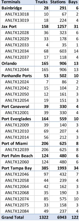
Table 7: Truck and Station Assignments

Terminals Trucks Stations Bays

Bainbridge 28 291 6 ANLTK13018 10 67 2 ANLTK13019 18 224 4 Jax Port 158 1257 31 ANLTK12028 36 323 6 ANLTK12029 33 178 6 ANLTK12033 4 35 1 ANLTK12034 68 603 14 ANLTK12037 17 118 4 Orlando 165 906 13 ANLTK12044 165 906 13 Panhandle Ports 53 502 10 ANLTK12024 7 86 2 ANLTK12042 15 104 2 ANLTK12050 12 161 3 ANLTK12054 19 151 3 Port Canaveral 39 330 4 ANLTK12001 39 330 4 Port Everglades 164 559 10 ANLTK12009 39 140 3 ANLTK12010 69 207 4 ANLTK12014 56 212 3 Port of Miami 206 625 8 ANLTK12039 206 625 8

Port Palm Beach 124 480 6

ANLTK12060 124 480 6

Port Tampa Bay 385 1993 34

ANLTK12046 97 432 7 ANLTK12058 44 239 4 ANLTK12064 42 162 3 ANLTK12068 35 190 3 ANLTK12074 85 575 10 ANLTK12075 33 158 3 ANLTK12084 49 237 4

Terminal Group Terminal Bays

Jax Port ANLTK12028 6

Orlando ANLTK12044 13

Port of Miami ANLTK12039 8

Port Palm Beach ANLTK12060 6

Port Tampa Bay ANLTK12046 7

Port Tampa Bay ANLTK12074 10

(23)

Visualization Interface

Together with MIT CTL’s research partners, the Computational and Visual Education (CAVE) Lab can be leveraged as an interactive decision-making space. By co-developing interactive visual analytics applications addressing specific, data-driven decision problems of our partners and presenting them in a way that leverages human perception and cognition, we aim to promote the effective future use of data and analytics by decision-makers at all levels across many organizations.

Applications built in the CAVE Lab are built on a framework that is open-sourced. The framework is designed to allow researchers to build analytical models in the programming language that works best for them. The application works with any model type and interacts with models through an API. This allows the framework to concentrate on the interactive decision making and data analytics needed to support decision makers.

This application was developed with support from FEMA with the goal to provide insights to aid in

response, but it is also envisioned as a useful tool to the private sector. The application has two views that are connected to the same scenario data. First, there is a map view that can be interacted with to create

scenarios, zoom, tilt, and show layers. Second, there is a dashboard view that provides summary statistics of the scenario that has been selected.

Map

The visualization of data from the simulation is handled by the application. There are several layers that can be visualized.

Available layers:

• Demand/Square mile: per capita gasoline consumption by ZIP Code Tabulation Areas (ZCTAs) • Demand Filled: percentage of demand met by the model

• Evacuation Routes: routes identified by the State of Florida

• Terminal Groups: consolidated groups of terminals with height representing the number of terminals at that location

• Terminals: location of the terminal with the height representing the number of bays at that location

(24)

• Stations: cluster view of retail station locations that changes the density of markers based on zoom level

Figure 7 shows the legend and the available layers that can be selected. Figure 8 is a zoomed in view of Tampa, Orlando, and Port Canaveral showing each of the terminals at these locations. The colors of the terminals and the stations that are assigned to them match the color of the terminal group. The station clusters change depending on the view level. Figure 9 shows the whole of Florida and the station assignments. The stations are colored the same color as their assigned terminal group.

(25)

Figure 8: Application Map Layers - Terminals and Stations with Detailed Clusters

(26)

Dashboard

Figure 10: Application Dashboard

Elements of the dashboard (shown in Figure 10): • Demand per area: map view

• Demand filled: map view

• System results: truck use and demand summary • Demand: summary by terminal group

• Truck use: by terminal group

The dashboard combines visualizations that summarize the scenario and the terminal groups. Demand and demand served are shown using both maps and bar charts. Summary statistics are available for the scenario and the terminal groups showing: the number of trucks available, trucks used, average fuel delivered, and total fuel delivered. In addition, the sunburst charts (see Figure 11), used in the dashboard, show how trucks spend their time in the model. There are sunburst charts for the whole network and for individual terminal groups.

The sunbursts charts capture the following values in units of time: • Closed: time the truck is not available to drive

(27)

• Station: time the truck is unloading fuel at the station • Terminal

o Terminal – Waiting for Gate to Open

o Terminal – In Gate Queue

o Terminal – At Gate

o Terminal – Waiting for Bay to Open

o Terminal – In Bay Queue

o Terminal – Filling Truck

Figure 11: Sunburst Chart

Model Input

In the CAVE Application, users can vary the parameters for each scenario created. They can change the parameters across the whole scenario or vary them by specific terminal groups. The demand is preloaded into the model with three variations: Lo, Med, Hi. It can be set for the whole scenario or just applied to a specific terminal group. For example, a user can create a scenario to simulate a hurricane strike at Jacksonville by applying the Hi demand variation to only that terminal group (See Figure 12).

(28)

Figure 13 shows the parameters that can be adjusted from within the CAVE Application. All parameters can be adjusted across the whole scenario (“Default) or for a selection of terminal groupings (“Specific).

The hours of operation can be varied for the trucks, gates, bays, and retail stations. The rates that trucks can pass through the gate, be filled, and emptied are also able to be changed. The capacity of trucks can also be altered.

The demand and number of trucks have an additional parameter. They can have a multiplier applied to them. Because the demand and number of trucks are given as pre-defined inputs to the model, the ability to be able to change them with a multiplier allows for flexibility while building scenarios. For example, to triple the number of trucks available at Port of Miami, the “Specific”

multiplier for the trucks would be changed to 3 and the Port of Miami would be selected. Alternatively, a

scenario could be created only considering the Orlando terminal with half of the usual demand. Setting the “Default” demand to 0 and the “Specific” demand for Orlando to 0.5 would create that scenario. This extreme flexibility is useful for exploring a wide range of possible scenarios.

(29)

Analysis

The analysis presented in this report is meant to be demonstrative, not comprehensive. There are many options that can be explored to reduce bottlenecks in the fuel system. These interventions can be put in place before a hurricane during Blue Sky operations or implemented during a hurricane event. Interventions will be discussed, and a subset of them will be explored below using the model and the CAVE Application to gain intuition about how various changes would improve outcomes.

Interventions

Interventions are changes to the system that can be made to improve the system’s performance. What are the interventions that the model can currently consider? What decisions/interventions could be made to change the output? Each intervention has a different impact and cost. Because the solve time for the model is a few seconds and the time to create new scenarios is less than a minute, the CAVE Application allows for the rapid exploration of the problem space and potential

interventions. There is no additional work to build data sets or code the model. Available interventions: (parameters to change)

● Number of trucks:

○ Hours of service (operating hours) ○ Weight limitations (truck capacity)

○ Improved carding systems at the terminal (trucks per terminal) ● Wait time at the gate

○ Add additional gates (gate rate)

○ Add an additional person to check trucks in while they wait (gate rate) ○ Improved gate access controls (gate rate)

● Time to fuel (filling rate)

○ Fueling login, payment, and configuration system are complicated and take a great deal of time – see updated system6_{pictured in Figure 14 (filling rate)}

○ Trucks with the ability to utilize parallel pump hoses could be prioritized (filling rate)

○ Diesel and gas available across all bays effectively increasing the number of bays (filling rate)

○ Adding bays (bays per terminal)

6_{https://www.opwglobal.com/docs/libraries/civacon/published-articles/delivering-the-correct-fuel.pdf}

Figure 14: New Fuel Delivery Monitoring System

(30)

● Time at the station

○ Road conditions (travel speed) ○ Faster emptying rates (empty rate)

As an example, the team was curious whether the number of trucks available in the model could support baseline demand. We used the multiplier parameter to triple the number of available trucks. There was no benefit to the baseline. That result aligned with conversations we had during field visits, suggesting the available truck fleet is optimized for normal operations.

The analysis that follows focuses on a small subset of these interventions.

Process Improvement Scenarios - “Building Intuition”

A. Increase the gate rate. A terminal could accomplish this by adding a second gate. In the model, the number of trucks processed per hour (i.e., the gate rate) would be doubled. Increase the number of trucks that can move through the gate from 10 trucks per hour to 20 trucks per hour. Most gates have a system where one truck can pass through the gate system at a time. It is composed of the main entry gate and a second gate. Only one of them can be opened at a time. To double the rate, a terminal could employ a faster gate, put a person at the gate to control the process, or add a second gate system to enter the terminal.

B. Increase the fill rate. A terminal could install an advanced check-in system at the bays. This would reduce the time spent filling a truck by increasing the gallons per hour of the fill rate. The observed and reported times for a truck to be filled at a bay ranged from 20 to 30 minutes. Part of the filling process involves logging into the bay, entering payment information, and programming the filling system. Assuming an automated system is employed, the total fill time for a truck could be reduced from the default of 25 minutes to 18.75 minutes per truck.

C. Improve both the gate rate and fill rate. A combination of A and B. Employ both of the above strategies at the same time.

D. Increase the hours of operation.

In addition to Intervention C, increase the hours of operation from 16 hours a day to 24 hours a day for trucks, stations, and terminals.

These interventions were tested against a Blue Sky scenario (Lo) and two Gray Sky scenarios where demand was increased (Med: x2 and Hi: x4) across the whole state and small stations were denied

(31)

For the analysis plan, we start with the baseline scenario to establish the “status quo” from which the interventions can be compared (1-3). Then we look to improve the throughput of the terminals by exploring how changes in the parameters impact the model (4-6). Afterward, we evaluate the impact of hurricane demand and how the added demand changes the value of the interventions that we identified (7-10). Lastly, we explore a new wrinkle where we extend the hours of terminals.

Table 9: Summary Statistics by Scenario

Table 9 shows the high-level results for the scenarios that we evaluated. The total demand and percentage of that demand that was filled are shown. The number of trucks utilized by the scenario is shown. Note that if a truck is filled, but not able to deliver its load before the station closes, that truck is not marked as used. The average time a truck spent in the various queues are shown as well. The last column is a sum of all the average queue and process times.

Scenarios

Baseline Scenarios

The network structure common across all the scenarios includes of the number of trucks and bays available at each terminal and the physical location of the stations and the terminals. Table 7 summarizes these characteristics at the terminal level. Table 10 summarizes these at the terminal group level. Jax Port and Port Tampa Bay have many bays and gates available, while Orlando and Port of Miami only have a single terminal with a single gate. This physical structure creates a bottleneck that we will explore in the scenarios.

No Description Dmd (M gal) % Dmd Filled Trucks Used Avg Fuel Delivered (gal) Avg Hr in Gate Queue Av Hr Bay Queue Avg Hr Filling Truck Avg Hr Total 1 Baseline: Lo demand 13.1 85% 1,268 18,084 7.25 0.68 0.94 8.87

2 Baseline: Med demand 34.9 63% 1,270 19,984 7.49 0.74 0.97 9.21

3 Baseline: Hi demand 69.8 37% 1,274 19,898 7.49 0.73 0.97 9.19

4 Intervention A: Lo demand 13.1 96% 1,322 21,384 6.98 0.98 1.15 9.10

5 Intervention B: Lo demand 13.1 85% 1,274 18,132 7.10 0.46 0.72 8.28

6 Intervention C: Lo demand 13.1 96% 1,322 21,573 6.19 0.71 0.90 7.80

7 Intervention A: Med demand 34.9 63% 1,272 19,961 7.48 0.73 0.97 9.19

8 Intervention A: Hi demand 69.8 37% 1,275 19,953 7.51 0.72 0.97 9.20

9 Intervention C: Med demand 34.9 80% 1,322 25,083 6.67 0.81 0.97 8.44

10 Intervention C: Hi demand 69.8 48% 1,322 25,113 6.67 0.79 0.97 8.43

11 Intervention D: Med demand 34.9 85% 1,322 27,731 8.46 0.90 1.09 10.46

12 Intervention D: Hi demand 69.8 53% 1,322 27,935 8.45 0.89 1.10 10.43

Terminal Group Trucks Stations Bays Gates

Bainbridge 28 291 6 2 Jax Port 158 1257 31 5 Orlando 165 906 13 1 Panhandle Ports 53 502 10 4 Port Canaveral 39 330 4 1 Port Everglades 164 559 10 3 Port of Miami 206 625 8 1

Port Palm Beach 124 480 6 1

Port Tampa Bay 385 1993 34 7

(32)

All scenarios also share a common demand portfolio. The demand is calculated at the station

location based on the number of people living in the ZCTA5 that the station is located in. From there, the stations are assigned to the closest terminal. A more in-depth discussion is available in the

Demand Scenarios section. Table 11 shows the breakdown of demand by terminal grouping.

It is important to notice that while there is more demand in Tampa Bay, Jax has almost the same number of terminals and about half as much demand. Miami and Orlando are also large population centers but have relatively fewer terminals. These types of structural features make a difference in network performance and will be highlighted below.

1. Baseline: Lo Demand

Given the data available and the assumptions made, we start by looking at the model behavior for a given Blue Sky Wednesday. Table 12 summarizes the output of that scenario. Several terminal groups do not perform well. Orlando and the Port of Miami only have a single terminal and are not able to serve over 30% of their demand. Palm Beach only met 82% of the demand it was trying to serve. Ports with more options for filling were able to get the trucks through their terminals and service demand.

Terminal Group Lo Med Hi

Bainbridge 267,103 593,289 1,186,574 Jax Port 1,564,961 4,107,077 8,214,143 Orlando 1,640,783 4,512,492 9,024,937 Panhandle Ports 503,889 1,277,506 2,555,032 Port Canaveral 384,191 991,313 1,982,624 Port Everglades 1,625,943 4,522,323 9,044,644 Port of Miami 2,058,057 5,251,870 10,503,768

Port Palm Beach 1,236,660 3,225,169 6,450,344

Port Tampa Bay 3,819,668 10,397,469 20,794,940

Demand

(33)

Table 12: Baseline - Lo Demand Summary

Terminal Bays Trucks Used % Dmd Filled Gate Queue Bay Queue Filling Truck Queue Total To Station Bainbridge 6 28 97% 0.21 0.81 1.74 2.76 3.01 ANLTK13018 2 10 92% 0.09 0.48 1.29 1.86 1.24 ANLTK13019 4 18 99% 0.28 1.00 1.99 3.26 3.99 Jax Port 31 158 96% 5.12 0.87 1.33 7.33 2.49 ANLTK12028 6 36 99% 2.60 1.14 1.78 5.52 3.45 ANLTK12029 6 33 97% 3.88 0.96 1.36 6.20 0.79 ANLTK12033 1 4 100% 0.02 0.79 1.56 2.37 0.77 ANLTK12034 14 68 92% 8.50 0.74 1.02 10.26 2.40 ANLTK12037 4 17 100% 0.57 0.71 1.50 2.78 4.47 Orlando 13 155 66% 7.82 0.27 0.43 8.52 0.48 ANLTK12044 13 155 66% 7.82 0.27 0.43 8.52 0.48 Panhandle Ports 10 53 100% 2.10 1.35 1.78 5.23 1.20 ANLTK12024 2 7 100% 0.13 0.64 2.08 2.85 2.69 ANLTK12042 2 15 99% 3.60 1.74 1.67 7.01 1.01 ANLTK12050 3 12 100% 0.23 1.18 1.84 3.25 1.11 ANLTK12054 3 19 100% 2.83 1.42 1.71 5.96 0.85 Port Canaveral 4 39 97% 5.33 1.15 1.61 8.09 1.91 ANLTK12001 4 39 97% 5.33 1.15 1.61 8.09 1.91 Port Everglades 10 164 96% 9.91 0.89 1.03 11.83 0.50 ANLTK12009 3 39 98% 7.95 1.12 1.21 10.28 0.54 ANLTK12010 4 69 93% 10.59 0.70 1.00 12.29 0.46 ANLTK12014 3 56 97% 10.44 0.96 0.94 12.34 0.52 Port of Miami 8 162 63% 7.45 0.30 0.42 8.17 0.27 ANLTK12039 8 162 63% 7.45 0.30 0.42 8.17 0.27

Port Palm Beach 6 124 82% 9.75 0.39 0.57 10.71 0.68

ANLTK12060 6 124 82% 9.75 0.39 0.57 10.71 0.68

Port Tampa Bay 34 385 92% 7.30 0.78 1.05 9.13 1.79

ANLTK12046 7 97 87% 8.94 0.49 0.74 10.16 2.02 ANLTK12058 4 44 97% 6.18 0.83 1.33 8.34 1.24 ANLTK12064 3 42 91% 2.87 0.89 1.17 4.94 3.62 ANLTK12068 3 35 98% 4.43 1.30 1.38 7.11 2.43 ANLTK12074 10 85 88% 10.26 0.63 0.83 11.72 1.15 ANLTK12075 3 33 100% 5.00 1.12 1.31 7.43 1.59 ANLTK12084 4 49 97% 7.30 0.87 1.27 9.43 1.08 122 1268 85% 7.25 0.68 0.94 8.87 1.25 Average Hours Spent

(34)

Table 12 also lists the average time a truck spent in the various queues. Gate queues saw the longest wait times. Truck congestion was observed at the gate if there were more trucks arriving than could get through the gate as well as if all the terminal’s bays were full fueling other trucks. Observing the total queue times, they ranged from 2.76 to 11.83 hours on average. Long weight times do not always indicate that demand will not be served. If the number of trucks needed to service the demand can be processed within the operating hours, then demand can be met. For example, Port Everglades has three terminals. They were able to process the necessary trucks to meet 96% of their demand but still had average wait times over 12 hours.

Recall the discussion in the Bottlenecks subsection of the Data section. In the (1) baseline scenario, the gate becomes a bottleneck if there are more than four bays in the terminal. Even with a surplus of trucks, demand will not be able to be fully met. Orlando and Port of Miami are two examples of this. The last column shows the average time for a truck to drive to its designated stations. The spread of these values demonstrates how population density affects the fuel network. At the Port of Miami. the average drive time is 0.27 hours. The stations are close to the terminal due to the fact Miami is

sandwiched between the sea and the Everglades. By contrast, the average drives from Bainbridge were over 3 hours. This is a rural part of the state and stations are farther apart. When the number of trucks is more constrained, the added travel time will come into play, and its effects can be seen in the model.

Figure 15: Baseline Dashboard

When using the CAVE Application, there is both a map view and a dashboard. Figure 15 shows the dashboard for the Baseline: Lo Demand scenario. The dashboard includes a global sunburst chart and individual charts for each of the terminal groups showing the terminal queues. There are also bar charts providing information about the demand served from each of the terminal groups. The

(35)

2. Baseline: Med Demand

In the second scenario, the demand increased, using the Med version. As the demand increases, smaller terminals perform worse. The Port of Miami and Orlando are meeting less than 40% of their demand. The average wait time for a truck increased by over 20 minutes. Here, the additional demand begins to impact the ability of larger stations to service their stations.

Table 13: Baseline - Med Demand Summary

3. Baseline: Hi Demand

The final baseline scenario increased demand even more. The average weight time was essentially the same, but the total demand met fell to 37%. If only 37% of the stations that get deliveries between 3 – 7 days per week can be met and the wait times remain static compared to the Med demand scenario, this implies that the queues are at close to capacity in the Med demand scenario. To resolve this, several interventions were investigated to identify positive changes to suggest in the fuel network. Terminal % Dmd Filled Gate Queue Bay Queue Filling Truck Queue Total Bainbridge 89% 0.29 0.77 1.47 2.53 Jax Port 86% 5.37 0.99 1.40 7.76 Orlando 36% 8.15 0.29 0.43 8.88 Panhandle Ports 96% 2.05 1.38 1.70 5.12 Port Canaveral 92% 5.35 1.19 1.71 8.25 Port Everglades 78% 10.32 0.95 1.05 12.32 Port of Miami 32% 7.30 0.29 0.42 8.01

Port Palm Beach 51% 9.71 0.38 0.58 10.67

Port Tampa Bay 71% 7.75 0.90 1.13 9.78

Total 63% 7.49 0.74 0.97 9.21 Average Hours Spent

(36)

Table 14: Baseline - Hi Demand Summary

Intervention Exploration

To increase the rate at which trucks can be loaded in the terminals, two interventions were

attempted. The first increased the speed trucks can enter the gate of the terminal, and the second decreased the time it takes to check-in at the bay.

4. Intervention A: Lo Demand

To add a second gate at the terminal the parameter for the gate rate is doubled from 10 trucks/hr to 20 trucks/hr.

Table 15 shows that the intervention succeeds in allowing all the terminals to serve over 90% of their demand. The gate queues are still over 10 hours at terminal groups with few gates, but the trucks are able to be filled and deliver their loads to the stations. Average bay queue times increased slightly as more trucks were able to access the bays due to the faster gate rate. The average time spent filling by a truck also increased. This is due to a few locations where trucks were able to return and be filled more than once per day.

Terminal % Dmd Filled Gate Queue Bay Queue Filling Truck Queue Total Bainbridge 60% 0.28 0.79 1.47 2.54 Jax Port 53% 5.44 0.97 1.40 7.80 Orlando 19% 8.09 0.29 0.44 8.82 Panhandle Ports 64% 2.08 1.38 1.70 5.16 Port Canaveral 61% 5.36 1.15 1.71 8.22 Port Everglades 44% 10.40 0.92 1.06 12.38 Port of Miami 16% 7.42 0.28 0.42 8.13

Port Palm Beach 26% 9.54 0.39 0.57 10.50

Port Tampa Bay 42% 7.70 0.91 1.13 9.73

(37)

Table 15: Intervention A- Lo Demand

5. Intervention B: Lo Demand

Automating check-in and programming at the bay reduces the time it takes to fill a truck. The fill rate for a truck was reduced from 25 minutes to 18.75 minutes per truck. This intervention was less

effective. The demand filled remained at 85%. The average time a truck spent in the bay queue dropped and relieved pressure on the gate queue, but it was not enough to move the needle for the whole system.

Table 16: Intervention B - Lo Demand

Port Palm Beach 95% 10.24 0.79 0.85 11.88

Port Tampa Bay 97% 5.31 1.18 1.31 7.81

Port Palm Beach 83% 9.83 0.28 0.44 10.55

Port Tampa Bay 92% 6.79 0.52 0.79 8.09

(38)

6. Intervention C: Lo Demand

Since both interventions produced a positive impact, it made sense to try them at the same time. Table 17 shows that the net result was similar to Intervention A, even as the wait times dropped. 96% of the demand was met with the Port of Miami seeing the most benefit. The wait times were reduced across the board. The fact that Intervention A and C can serve the same percentage demand, even with reduced wait times, reminded the research team of a quote from a fuel distributor in Florida who said, “I don’t mind a two-hour line, as long as I can get product”. This is a good reminder that even if an intervention yields a better result, there may not be a need in the market place for it. That is especially true if the intervention is costly.

Table 17: Intervention C - Lo Demand

Deeper Analysis

The two most promising interventions were (A) increasing the gate rate and the combination of A and B (C). We tested these under the all the demand variations to see how sensitive the interventions were to the level of demand. Perhaps Intervention C did not perform better than Intervention A under Blue Sky conditions but may prove more valuable during hurricane conditions.

7. Intervention A: Med Demand

Once the demand was increased to levels that might be experienced during a hurricane, Intervention A performed similarly to the second baseline scenario with the same level of demand. Wait times were only slightly lower. The reduced bottleneck at terminal gates kept trucks available at the bays, but the filling rate and the number of bays became the new bottleneck.

Port Palm Beach 95% 10.00 0.63 0.83 11.45

Port Tampa Bay 97% 3.82 0.82 0.99 5.64

(39)

Table 18: Intervention A - Med Demand

8. Intervention A: Hi Demand

The Hi demand variation had a similar result. It resembled the (3) baseline Hi demand scenario. This level of demand overwhelmed the fuel network as in the (7) Intervention A: Med demand scenario.

Table 19: Intervention A - Hi Demand

9. Intervention C: Med Demand

Since Intervention A was not successful in hurricane conditions, the next two scenarios applied both Intervention A and B to the two hurricane demand variations.

Port Palm Beach 50% 9.62 0.43 0.57 10.61

Port Tampa Bay 71% 7.69 0.89 1.13 9.71

Port Palm Beach 26% 9.70 0.41 0.58 10.69

Port Tampa Bay 42% 7.72 0.91 1.13 9.76