Methods and software tools for design evaluation for population pharmacokinetics-pharmacodynamics studies.: Softwares for design evaluation in population PKPD

HAL Id: inserm-00978789

https://www.hal.inserm.fr/inserm-00978789

Submitted on 14 Apr 2014

HAL is a multi-disciplinary open access

archive for the deposit and dissemination of sci-entific research documents, whether they are pub-lished or not. The documents may come from teaching and research institutions in France or abroad, or from public or private research centers.

L’archive ouverte pluridisciplinaire HAL, est destinée au dépôt et à la diffusion de documents scientifiques de niveau recherche, publiés ou non, émanant des établissements d’enseignement et de recherche français ou étrangers, des laboratoires publics ou privés.

Methods and software tools for design evaluation for

population pharmacokinetics-pharmacodynamics studies.

Joakim Nyberg, Caroline Bazzoli, Kay Ogungbenro, Alexander Aliev, Sergei

Leonov, Stephen Duffull, Andrew Hooker, France Mentré

To cite this version:

Joakim Nyberg, Caroline Bazzoli, Kay Ogungbenro, Alexander Aliev, Sergei Leonov, et al.. Methods and software tools for design evaluation for population pharmacokinetics-pharmacodynamics studies.: Softwares for design evaluation in population PKPD. British Journal of Clinical Pharmacology, Wiley, 2015, 79 (1), pp.6-17. �10.1111/bcp.12352�. �inserm-00978789�

1

Methods and software tools for design evaluation for population

pharmacokinetics-1 pharmacodynamics studies 2 3 Authors 4

Joakim Nyberg (1), Caroline Bazzoli (2), Kay Ogungbenro (3), Alexander Aliev (4), Sergei Leonov (5), 5

Stephen Duffull (6), Andrew C. Hooker (1), France Mentré (7) 6

(1) Department of Pharmaceutical Biosciences, Uppsala University, Uppsala, Sweden; 7

(2) Laboratoire Jean Kuntzmann, Département Statistique, University of Grenoble, France ; 8

(3) Centre for Applied Pharmacokinetic Research, School of Pharmacy and Pharmaceutical Sciences, 9

University of Manchester, Manchester, United Kingdom; 10

(4) Institute for Systems Analysis, Russian Academy of Sciences, Moscow, Russia; 11

(5) AstraZeneca, Wilmington, DE, USA; 12

(6) School of Pharmacy, University of Otago, Dunedin, New Zealand; 13

(7) INSERM U738 and University Paris Diderot, Paris, France; 14

15

Submitting Author and Corresponding Author

16

France Mentré, france.mentre@inserm.fr 17

18

Running head: Softwares for design evaluation in population PKPD

19

Keywords: optimal design, population design, Fisher information matrix, nonlinear mixed effect

20

models, population PKPD, PFIM, PkSaMp, PopDes, POpED, POPT. 21

Word count: 3800

22

Numbers of tables and figures: 5 tables and 2 figures

2

Summary

24

Population Pharmacokinetic (PK)-Pharmacodynamic (PD) (PKPD) models are increasingly used in drug 25

development and in academic research. Hence designing efficient studies is an important task. 26

Following the first theoretical work on optimal design for nonlinear mixed effect models, this 27

research theme has grown rapidly. There are now several different software tools that implement an 28

evaluation of the Fisher information matrix for population PKPD. We compared and evaluated five 29

software tools: PFIM, PkStaMP, PopDes, PopED, and POPT. The comparisons were performed using 30

two models: i) a simple one compartment warfarin PK model; ii) a more complex PKPD model for 31

Pegylated-interferon (peg-interferon) with both concentration and response of viral load of hepatitis 32

C virus (HCV) data. The results of the software were compared in terms of the standard error values 33

of the parameters (SE) predicted from the software and the empirical SE values obtained via 34

replicated clinical trial simulation and estimation. For the warfarin PK model and the peg-interferon 35

PKPD model all software gave similar results. Of interest it was seen, for all software, that the simpler 36

approximation to the Fisher information matrix, using the block diagonal matrix, provided predicted 37

SE values that were closer to the empirical SE values than when the more complicated approximation 38

was used (the full matrix). For most PKPD models, using any of the available software tools will 39

provide meaningful results, avoiding cumbersome simulation and allowing design optimisation. 40

3

Introduction

42

Estimation of pharmacokinetic (PK) parameters for an individual using nonlinear regression 43

techniques started in the 1960’s, followed by estimation of dose-response and of pharmacodynamics 44

(PD) models. At around the same time mathematical approaches to defining the problem of optimal 45

design for parameter estimation in nonlinear regression was addressed (1-3). However this did not 46

reach the PK literature until some 20 years later (4). The problem was not only to draw inference 47

from data but also to define the best design(s) for estimation of parameters using maximum 48

likelihood or other estimation methods. For this purpose, the Fisher Information matrix (FIM) was 49

used to describe the informativeness of a design, i.e. how much information the design has in 50

relation to parameter estimation. Typically in PK the FIM is summarized by its determinant and 51

maximising the determinant, termed D-optimality, is equivalent to minimising the asymptotic 52

confidence region of the parameters, i.e. getting the most precise parameter estimates (5-9). 53

However, beyond theoretical developments, a limitation of individualised optimised designs of PKPD 54

studies is that those designs do not acknowledge population information and hence cannot have 55

fewer sampling times per individual than parameters to estimate. In addition, optimal designs with a 56

large number of observations per patient will have replicated optimal sampling times; which were 57

not favoured by pharmacologists interested in exploring complex PK models. Some later work also 58

explored Bayesian designs, where a priori distributions of the parameters were considered, and 59

individual parameters were estimated using maximum a posteriori probability (MAP). Optimal 60

designs for MAP estimation optimise individual designs given prior population information and are 61

suitable for e.g. therapeutic drug monitoring designs (10, 11). Since 1985, the software Adapt 62

(https://bmsr.usc.edu/software/adapt/) has included methods for optimal design in nonlinear 63

regression using several criteria for MAP estimation. 64

The population approach was introduced by Sheiner et al. (12) for PK analyses in the late 1970’s and 65

since the 1980’s there has been a large increase in the use of this approach as well as extensions to 66

PKPD. Estimation was mainly based on maximum likelihood using nonlinear mixed effects models 67

(NLMEM) thanks to the software NONMEM. To our knowledge the first article studying the impact of 68

a ‘population design’ on properties of estimates was performed in early 1990’s by Al Banna et al. (13) 69

for a population PK and a population PKPD example. In this work the author used clinical trial 70

simulation (CTS) to explore possible designs. The authors studied the influence of the balance of 71

number of patients, number of sampling times and locations of the sampling times on the precision 72

of the parameter estimates. Several papers, all using CTS, were published (14-16) showing that some 73

designs could be rather poor, and that very sparse designs also performed poorly. The FDA’s 74

4 Guidance for Industry Population Pharmacokinetics (17) from 1999 includes a specific section on 75

design, and suggests that simulation, based on preliminary information, should be performed to 76

“anticipate certain fatal study designs, and to recognize informative ones”. 77

Using CTS for design evaluation requires a large number of data sets to be simulated and then fitted 78

under each proposed design which is computationally expensive. However, since CTS is a user driven, 79

heuristic approach, then it can miss important regions of the design space because only a fixed 80

number of designs are investigated. Subsequently it was suggested to use the FIM in NLMEM to 81

predict asymptotic standard errors (SE) and define optimal designs without the need for intensive 82

simulations. Because the population likelihood has no closed-form expression the proposed 83

approach for defining the population FIM was to use a first-order linearisation of the model around 84

the random effects (which is the same as used for the first-order (FO) estimation methods). This 85

approximation results in a mixed effect model where the random effects enter the model linearly 86

(rather than nonlinearly) and hence has properties that are similar to linear mixed effects model. The 87

expression for the population FIM was first published in Biometrika in 1997 (18). In this work the FIM 88

was derived for a population PK example and an algorithm was proposed to optimise designs based 89

on the population FIM. This paper launched the new field of optimal design for nonlinear mixed 90

effects models. It has been quoted in the section ‘other influential papers of the 1990’s’ in a review 91

in Biometrika (19). 92

Since 1997 several methodological papers from various academic teams have published different 93

extensions, for instance robust designs, sampling windows, compound designs, multiple response 94

models, methods for discrete longitudinal data, and other approximations of the FIM, etc. Most 95

importantly, the derivation of the expression of the FIM was implemented in several software tools, 96

the first one PFIM (20) in 2001 appeared simultaneously in both R (http://www.r-project.org/) and 97

Matlab (http://www.mathworks.fr/products/matlab/). This was followed by POPT (21), and later to 98

incorporate an interface version WinPOPT, PopED (22), PopDes (23) and PkStaMp (24). There are 99

now five different software tools, all implementing the first-order approximation, with some tools 100

implementing one or several other approximations. These tools for designing population PKPD 101

studies are gaining popularity. In a recent study performed among European Federation of 102

Pharmaceutical Industries and Associations members’ (25), it was found that 9 out of 10 103

pharmaceutical companies are using one of these software tools for design evaluation or 104

optimisation, mainly in phases I and II. 105

5 The computation of the FIM is complex and depends on the numerical implementation. The purpose 106

of the present work was therefore to compare the results provided by those different software tools 107

in terms of FIM and predicted SE values. The same basic approximations were used in each software, 108

and the comparison was performed for two examples: (1) a simple PK example described by a one-109

compartment model with first-order absorption and linear elimination and (2) a more complex PKPD 110

example where the PD component is defined by a system of nonlinear ordinary differential equations 111

(ODE). The objective was to explore the results from different software tools and to compare results 112

against those obtained using CTS. We wanted to show the user community that similar results would 113

be obtained with any software tool although programmed in different languages and by different 114

authors. This was also studied in the case of a multiple responses ODE model where the numerical 115

imbrication between ODE solver and numerical differentiation is complex. The results were provided 116

by the software developers, all authors of this article, who were given the equations of the models, 117

the values of the parameters and the designs to be evaluated. Results were compared to those 118

obtained by CTS. 119

The article is organized as follows: first the description of the population FIM for NLMEM, second a 120

description of the various software tools, and then an evaluation of the two examples. As no design 121

optimisation was performed in the present study, no optimisation characteristics or algorithms are 122

described. 123

124

Statistical methods for design in NLMEM

125

A design for a multi-response NLMEM is composed of

N

subjects each with an associated 126

elementary design

ξ

_i(i=1,...,N). Hence a design for a population of

N

subjects can be described 127 as 128

(

ξ

1

,...,

ξ

N

)

Ξ =

(1) 129

Each elementary design

ξ

_i can be further divided into sub-designs 130

(

1

,

,

)

i i iK

ξ

=

ξ

…

ξ

(2)

131

with

ξ

_ik, k=1,...,K being the design associated with the kth response. (e.g. drug concentration, 132

metabolite concentration, effect). It may thus be possible to have all responses measured at different 133

times, termed an unbalanced design. 134

6 A design for subject i at a response k =1,...,K often consists of several design variables which might 135

be constant between observations, e.g. the drug dose, or vary between observations, e.g. the times 136

at which the response variable is measured. 137

An elementary design

ξ

_l can be the same within a group

l

of

N

_lsubjects (l=1,…,L). Using a

138

similar notation for the complete population design

Ξ

in a limited number of L groups of different 139

elementary designs gives: 140

[

] [

]

(

ξ

1,N1 ,...,

ξ

L,NL

)

Ξ = (3)

141

where the total number of subjects in the design,

N

, is equal to the sum of the subjects in the L

142

elementary designs. At the extreme, each subject may have a different design, L = N, or each subject 143

may have the same design, L = 1. 144

In a NLMEM framework with multiple response, the vector of observations

Y

_i for the ith subject is 145

defined as the vector of K different responses: 146

Y

_i

=

_



y

_iT₁

,

y

_iT₁

,

…

,

y

_iKT



_

T (4)

147

where y_ik,k =1,…,K is the vector of nik observations for subject i and response k modelled as

148

(

)

(

)

f

,

h

,

,

ik k i ik k i ik ik

y

=

θ ξ

+

θ ξ ε

(5) 149

where fk(.) is the structural model for the k th

response,

θ

_i is the ith subject’s parameter vector, hk(.) is

150

the residual error model for response k, often additive (h=

ε

_ik), proportional (h=

f

k

( )

⋅

ε

ik) or a

151

combination of both,

ε

_ik is the residual error vector for response k in subject i. In this paper additive 152

(homoscedastic) or proportional (heteroscedastic) error models will be used in the examples so that 153

only one residual variance parameter is defined for each response. To simplify notation we assume 154

that

ε

_ikare normally distributed and independent between responses (which is not necessary, see 155

e.g. (26, 27)) with mean zero and variance Σk=diag(

σ

_k2). The individual parameter vector

θ

_i, with

156

parameter(s) that might be shared between responses, is described as 157

(

)

g

,

i

b

i

θ

=

β

(6) 158

7 where

β

is the u-vector of fixed effects parameters, or typical subject parameter and bi, the vector

159

of the

v

random effects for the subject i defining the subject deviation from the typical value of the 160

parameter. We assume that bi is normally distributed with a mean of zero and a covariance matrix

161

Ω of size × . Again, to simplify notation we assume a diagonal (which is not necessary, see e.g. 162

(18, 27-29)) interindividual covariance matrix (Ω) with diagonal elements (

ω

₁2,...,

ω

_v2). The vector of 163

population parameters is thus defined as 164

[ ]

2 2 2 2 1 1 , , ,..., _v, ,..., _K

ψ

₌

β λ

₌_

β ω

ω σ

σ

_ (7) 165

where

λ

=_

ω

₁2,...,

ω σ

_v2, ₁2,...,

σ

_K2_ is the vector of all variance components. 166

The population Fisher information matrix

FIM

(

ψ

,

Ξ

)

for multiple response models with the 167

population design

Ξ

ΞΞ

Ξ

is given by: 168

(

,

)

2

L

(

,

Y

_T

)

FIM

ψ

E

ψ

ψ ψ



_∂



Ξ =



_

−



_

∂ ∂





(8) 169

where

L

(

ψ

,

Y

)

is the log-likelihood of all the observations Y given the population parameters

ψ

.

170

Assuming independence across subjects, the log-likelihood can be defined as the sum of the 171

individual contribution to the log-likelihood:

(

)

(

)

1 , , N i i L

ψ

Y L

ψ

Y =

=

_∑

. Therefore, the population

172

Fisher information matrix (calculated using the second derivative of the log-likelihood) for N subjects 173

can also be defined as the sum of the N elementary information matrices

FIM

(

ψ ξ

,

_i

)

computed for 174 each subject i: 175

(

)

(

)

1 , , N i i FIM

ψ

FIM

ψ ξ

= Ξ =

∑

(9) 176

In the case of a limited number of L groups (where each individual in a group share the same design), 177

as in Equation (3), the population FIM is expressed by: 178

8

(

)

(

)

1 , , L l l l FIM

ψ

N FIM

ψ ξ

= Ξ =

∑

(10) 179 180

For one subject, given the design variables

ξ

_iand the NLMEM model, the FIM is a block matrix 181 defined as: 182

(

)

1 FIM , 2 i A C C B ψ ξ =       (11) 183 where

(

,

)

1

2

i

FIM

β ξ

=

A

is the block of the Fisher matrix for the fixed effects

β

and 184

(

)

1

,

2

i

FIM

λ ξ

=

B

is the block of the Fisher matrix for the variance components

λ

. 185

When a standard FO approximation of the model is performed (see appendix), then the distribution 186

of the observations in patient i with design ξi is approximated by

Y

i

~ N

(

E V

i

,

i

)

. Expressions for the

187

population mean

E

_iand population variance

V

_i are given in the appendix. Then the following 188

expression for blocks A, B and C are obtained (18, 30, 31), ignoring indices i for simplicity : 189 1 1 1 2 tr T pq p q p q E E V V A V V V

β

−

β

β

−

β

−   ∂ ∂ ∂ ∂ ≅ + _ _ ∂ ∂ _∂ ∂ _ with

p q

,

=

1..dim

( )

β

190 1 1 pq p q

V

V

B

V

V

λ

−

λ

−

∂

∂

≅

∂

∂

with

p q

,

=

1..dim

( )

λ

(12) 191 1 1

tr

pq p q

V

V

C

V

V

λ

−

β

−



_∂

_∂



≅



_



_

∂

∂





with

p

=

1..dim

( )

λ

,

q

=

1..dim

( )

β

192

193

This expression of the FIM (eq. 12) will be referred to as the full FIM in this paper. 194

If the approximated variance V is assumed independent of the typical population parameters

β

, the 195

matrix C will be zero and the matrices A and B will instead be defined as: 196 1 2 T pq p q E E A V

β

−

β

∂ ∂ ≅ ∂ ∂ with

p q

,

=

1..dim

( )

β

(13) 197

9 1 1 pq p q

V

V

B

V

V

λ

−

λ

−

∂

∂

≅

∂

∂

with

p q

,

=

1..dim

( )

λ

198 199

which will be termed the block diagonal FIM in the following. The explicit formula for

FIM

(

β ξ

,

i

)

200

using the block diagonal form is given in the appendix. More information about the derivation of the 201

FIM or other approximations are reported in (27, 28, 30, 32-34). 202

203

Software description

204

There are presently five software tools that implement experimental design evaluation and 205

optimisation of the FIM for multiple response population models. The five software tools are (in 206

alphabetical order) : PFIM (35), PkStaMp (24), PopDes (23), PopED (27, 31) and POPT (21). Four of 207

them have been developed by academic teams. 208

PFIM (Population Fisher Information Matrix) is the only tool that is using the software R, the other 209

software packages have been developed under the numerical computing environment MATLAB. The 210

first version of PFIM appeared in 2001 and since this date several releases have been issued. It is 211

available at www.pfim.biostat.fr. A graphical user interface (GUI) package using the R software 212

(PFIM Interface) is also available but does not include recent methodological developments. 213

Pk StaMP (Pharmacokinetic Sampling Times Allocation – Matlab Platform) is a library compiled as a 214

single executable file which does not require a MATLAB license. The developers can share the stand-215

alone version with anyone interested. PopDes (Population Design) has been developed at the 216

University of Manchester and this application software is available at www.capkr.man.ac.uk/home 217

since 2007. PopED (Population optimal Experimental Design), freely available at poped.sf.net, 218

consists of two parts, a script version, responsible for all optimal design calculations, and a GUI. The 219

script version can use either MATLAB or Freemat (http://www.freemat.sf.net)(a free alternative to 220

MATLAB) as an underlying engine. Some advanced PopED features such as automatic and symbolic 221

differentiation, Laplace approximation of Bayesian criteria and mode base linearisation are not 222

available in FreeMat, however all features presented in Table 1 are available in PopED using either 223

FreeMat or Matlab. POPT (Population OPTimal design) was developed from PFIM (MATLAB) in 2001 224

and is constructed as a set of MATLAB scripts. POPT requires MATLAB and can run on FreeMat. This 225

tool can be downloaded on the website www.winpopt.com. All the software tools run on any 226

common operating system platform (e.g. Windows, Linux, Mac). 227

10 228

Comparison of software for design evaluation

229

As we focus on design evaluation and not design optimisation, we first compared the software tools 230

with respect to a) required programming language, b) availability, c) library of PK and PD models, and 231

ability to deal with: d) multiple response models, e) models defined by differential equations, e) 232

unbalanced multiple response designs, f) correlations between random effects and/or residuals, g) 233

models including inter-occasion variability, h) models including fixed effects for the influence of 234

discrete covariates on the parameters, i) computation of the predicted power. Table 1 is a summary 235

of the comparison of the software with respect to these different aspects. Globally, for all software 236

tools, the library of PK models includes one, two and three compartment models, with bolus, 237

infusion and first-order (e.g. oral) administration, after a single dose, multiple doses and at steady 238

state. PK models with first-order elimination and models Michaelis-Menten elimination are available. 239

Regarding PD models, immediate linear and Emax models and turnover response models are 240

available. 241

Over recent years, those tools have included various improvements in terms of model specification 242

and calculations of the FIM. For all of them, design evaluation can be performed for single or multiple 243

response models either using libraries of standard PK and PD models or using a user-defined model. 244

For the latter, regardless of the software used, the model can be written using an analytical form or 245

using a differential equation system. In the case of multiple response models, population designs can 246

be different across the responses for all the software. Regarding the calculations of the information 247

matrix, the majority of the software can handle either a block diagonal Fisher information matrix 248

(block FIM) or the full matrix (full FIM). Otherwise, only PopDes and PopED allow for calculations for 249

a model with both correlation between random effects (full covariance matrix Ω) and correlation 250

between residuals (full covariance matrix Σ), PKStamp allows full covariance matrix Ω. It is possible in 251

PFIM, PopDes and PopED to use models with inter-occasion variability (IOV) and models including 252

fixed effects for the influence of discrete covariates on the parameters. The computation of the 253

predicted power of the Wald test (30, 36) for a given distribution of a discrete covariate can be 254

evaluated in PFIM, PopDES and PopED frameworks. 255 256 257 258 259 260

11

Examples

261

Two different examples were used to illustrate the performance of the five population design 262

software tools. Note that the examples evaluated the prediction for a given design, by evaluating the 263

FIM and the predicted asymptotic SEs, without design optimisation. This was done to evaluate the 264

core calculations of the FIM. The FIM is evaluated with the full and the block diagonal derivation (eq. 265

12, 13) with the different software tools. 266

In the first example a one compartment PK model (based on a warfarin PK model) with first-order 267

absorption was used (35). The design of that study consisted of 32 subjects with a single dose of 70 268

mg (a dose of 1mg/kg and a weight of 70 kg), and with 8 sampling times post-dose (in hours): 269

[

]

(

ξ

1

,

N

1

)

(

ξ

1

,32

)

Ξ =

=

270

( ) (

)

1

t

i

0.5,1, 2,6, 24,36,72,120

ξ

=

=

271

The residual error model was proportional (h =

f

⋅

ε

) with a coefficient of variation of 10% ( 272

2

0.01

σ

= ) and exponential random effects were assumed for all parameters (

g

=

β

_e

bi_{). Table 2}

273

reports the model parameters and their values. The dose and design are based on (34, 37). 274

For the second example a multiple response PKPD model with repeated dosing was selected with the 275

same design across responses (38). The model describes hepatitis C virus (HCV) kinetics, or more 276

specifically, the effect of peg-interferon dose of 180 μg/week administered as a 24 hour infusion 277

once a week for 4 weeks. The same sequence of 12 sampling times for both PK and PD 278

measurements (in days, post-first-dose) was used for 30 subjects: 279

{

}

(



ξ ξ

_PK, _PD ,N_PKPD

)

(

ξ ξ

_PK, _PD, 30

)

Ξ = _{ } = 280

( ) (

0,0.25,0.5,1, 2,3, 4,7,10,14, 21, 28

)

PK PD

t

i

ξ

=

ξ

=

=

281

The HCV model is described by the following system of ODEs: 282

12

( ) ( )

( )

( )

( )

( )

( )

(

( )

)

( )

( ) ( )

( )

,

0

0

,

0

0

,

0

,

a a e

dX

k X t

r t

X

dt

dA

k X t

k A t

A

dt

dT

c

s T t

eW t

d

T

dt

pe

dI

eW t T t

I t

dt

δ

δ

= −

+

=

=

−

=

= −

+

=

=

−

( )

( )

_{( )}

_{( )}

_{( )}

50

0

1

,

0

( )

n n n

sep dc

I

p e

C t

dW

sep dc

p

I t

cW t

W

dt

C t

EC

c e

δ

δ

δ

δ

−

=





₋





=

_

−

_

−

=

+





283 284

where

C t

( )

=

A t V

( )

_d is the drug concentration at time t and r(t) is the constant infusion rate. The 285

viral dynamics model considers target cells, T, productively infected cells, I and viral particles, W. 286

Target cells are produced at a rate s and die at a rate d. Cells become infected with de-novo infection 287

rate e. After infection, these cells are lost with rate δ. In the absence of treatment, virus is produced 288

by infected cells at a rate p and cleared at a rate c, for more details see (38, 39). The model for each 289

response in subject i is defined as 290

( )

( )

₍

( )

₎

, 10 , 10

log

log

i PK i iPK i PD i iPD

y

C t

y

W t

ε

ε

=

+

=

+

291

An additive error model was assumed for both PK and PD (log viral load) compartments from which 292

observations were drawn with a standard deviation of 0.2. Some of the parameters in the model are 293

fixed (p, d, e, s). For the other seven parameters (ka, ke, Vd, EC50, n,

δ

, c), log transformation was

294

made with additive random effects on the log fixed effect with a variance ω2 of 0.25. All parameters 295

and their values are listed in Table 3. 296

297

Methods

298 299

For each example using each software tool, we computed the FIM based on the FO linearisation, 300

given the parameters and the design. We used both the block-diagonal and the full FIM (not available 301

in POPT). From the FIM, we computed the predicted SE values for each parameter and the 302

13 information D-criterion which is defined as the determinant of the FIM to the power of one over the 303

number of parameters:

FIM

1/dim( )ψ . 304

To investigate the FIM predictive performance, the empirical SE values were also estimated using 305

CTS. More precisely, for each example, multiple data sets were simulated and then fitted using the 306

Stochastic Approximation Expectation Maximisation (SAEM) algorithm in MONOLIX 2.4 307

(www.lixoft.eu) and, for the PK example also with the FOCEI algorithm in NONMEM 7 308

(http://www.iconplc.com/technology/products/nonmem/). Empirical standard errors were derived 309

from the estimated parameters. The empirical D-criterion was computed from the normalized 310

empirical variance-covariance matrix of all estimated parameters,

( )

( ) 1/dim 1

cov

ψ

− ψ . Because the 311

CTS was much more time consuming for the HCV PKPD model, we did not perform the estimation 312

with NONMEM and we did only 500 replicates, whereas we simulated 1000 replicates for the 313

warfarin PK model. 314

For the CTS, to compute the empirical covariance matrix, the full variance-covariance matrix of all the 315

estimated vectors was computed, not as two separate blocks for fixed effects and random 316 components. 317 318 Results 319 320

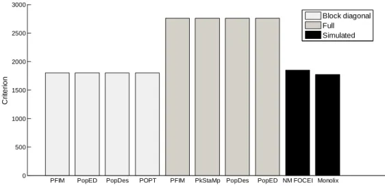
For the PK model, the results show no differences between the optimal design software tools when 321

evaluating the FIM using the block diagonal and full form. In the same way, all software reported the 322

same expected D-criterion (Figure 1), and the same expected relative standard errors (RSE) values 323

expressed in % (Table 4). 324

In this example, the block diagonal FIM calculations gave an expected D-criterion that was very 325

similar to the observed D-criterion based on the inverse of the empirical covariance matrix (Figure 1). 326

However, for all software, the block diagonal D-criterion is slightly smaller than the NONMEM FOCEI 327

based criterion. Note that the result from MONOLIX is lower than the expected D-criterions, in line 328

with theoretical expectations the Cramer-Rao inequality (FIM is an asymptotic upper bound on the 329

information). The full FIM predicts considerably more information compared to the simulations 330

(expected D-criterions are larger than the observed values), and predicts total information that is 331

farther from the empirical values than the block diagonal calculations. The same trends are evident 332

when looking at the RSE values, reported in Table 4. Good agreement between the CTS and the block 333

14 diagonal FIM was found, while the full FIM predicted considerably higher precision in

β

_Ka and

β

_CL/F 334

. 335

For the more complicated PKPD model, results are summarized In Figure 2 and Table 5 where RSE (%) 336

are reported. The D-criterion reveals negligible differences between any of the software (Figure 2) 337

and also almost no difference between predicted SE values (Table 5). In this example, as in the PK 338

example, using the block diagonal FIM gave D-criterion predicted values that were very similar to the 339

D-criterion based on the inverse of the empirical covariance matrix (Figure 2). The full FIM predicts 340

considerably more information compared to the simulations (expected D-criterions larger than the 341

observed values) and predicts total information (D-criterion) that is farther from the empirical values 342

than the block diagonal calculations. The same trends are evident when looking at SE values for each 343

parameter (Table 5). We found good agreement between CTS and the block diagonal FIM, while the 344

full FIM predicted higher precision in numerous parameters than observed. 345

346

15

Discussion

348

The first statistical developments for the evaluation of the FIM for NLMEM to compare and evaluate 349

population designs without simulation were performed in the late 90’s. Since then, five different 350

software tools have been developed. We have compared these tools in terms of design evaluation. 351

Optimisation was not considered in the present work. It should be noted that most software are 352

under active development with regular addition of new features. 353

We compared the expression of the FIM computed by the five different optimal design software 354

packages for two examples. The first example was a simple PK model for which the algebraic 355

solution could be written analytically. When using the same approximation, all optimal design 356

software packages achieved the same D-efficiency criterion and predicted RSE values (%). The second 357

example was more complex, had two responses (both PK and PD measurements) and the model was 358

written as a series of five differential equations. For this example, the D-criterion and RSE 359

comparisons revealed negligible differences between software. The differences could potentially be 360

explained by the use of different differential equation solvers, methods of implementing multiple 361

response calculations, methods for computing numerical derivatives, tolerance levels for ODEs and 362

numerical implementations of e.g. matrix inverses and solving of linear systems, etc. These small 363

differences could be seen even across the MATLAB computations of the FIM. In this work we did not 364

impose the same implementation of the various steps across software, hence the importance of the 365

present comparison. 366

367

In both examples the expected SE values from the block diagonal FIM were close to the empirical SE 368

values obtained from CTS. The runtimes for all software tools were a few seconds compared to 369

minutes (warfarin example) or days (HCV example) for the CTS evaluation. Although computational 370

speed has increased dramatically since the 1990’s, a significant speed advantage is seen with the 371

developed software tools even without considering design optimisation. For instance for the HCV 372

PKPD model the CTS took several days for one design, so that optimization of doses and sampling 373

times would be difficult. 374

In both examples investigated, the block diagonal FIM calculations give an expected D-criterion that 375

is very similar to the observed D-criterion based on the inverse of the empirical covariance matrix 376

and RSE(%) values for parameter match well. In contrast, the full FIM predicts more information 377

compared to the simulations (expected D-criterions larger than the observed values). More 378

discussion on the assumptions beyond the block or full matrix can be found in (33) together with 379

16 suggestions of other stochastic approaches. It seems that when using a FO approximation for 380

computation of the FIM, linearisation around some fixed values for the fixed effects which are then 381

no longer considered as estimable parameters and therefore corresponds to the block diagonal 382

matrix, provides the best approach. Also higher order approximations to the FIM are available that 383

may give better prediction of RSE(%) values (27). 384

Results using the simple FO approximation and the block diagonal FIM are very close to those 385

obtained by CTS using both FOCEI and SAEM estimation methods in the two examples. However, 386

since the expected FIM calculation is computing an asymptotically lower bound of the covariance of 387

the parameters, and the calculations are based on approximations, the authors suggest that a CTS 388

study of the proposed final design be performed in order to evaluate the likely performance of the 389

design in the setting in which it is proposed to be used. Since this would be a single CTS at a specified 390

design then this should not be computationally onerous compared to attempting to “optimise” 391

designs using CTS. In addition, using a CTS study of the final design makes it possible to assess the 392

bias which is not evaluated by the FIM. 393

In this first comparison between the software, we did only design evaluation for continuous data and 394

using the simpler FO approximation of the FIM. This first step was necessary before the next work 395

where we will compare results of design optimisation. Indeed now that we know that similar 396

criterion across software are obtained, we can compare the rather different optimisation algorithms 397

implemented. In principle any design variable that is present in the model can be optimised within an 398

optimal design framework. Examples of design variables that can be optimised are measurement 399

sampling times, doses, distribution of subjects between elementary designs, number of 400

measurement samples in an elementary design, etc. How this is done and which design variables can 401

be optimised varies between software, but the independent variable (e.g. measurement sampling 402

times) and the group assignment can be optimised in all software presented in this paper. Results will 403

depend on the assumptions about the model and the parameter values, so that sensitivity studies 404

should be performed to implement ‘robust’ designs, i.e. designs that are robust to the assumed a 405

priori values of the parameters. Approaches for design optimisation using a priori distribution of the

406

parameters were suggested and implemented for standard nonlinear regression and extended to 407

population approaches and should also be compared in further studies. 408

In conclusion, optimal design software tools allow for direct evaluation of population PKPD designs 409

and are now widely used in industry (25). Choice of software can depend on what platform the user 410

has available and what features they are looking since the FIM calculation in the different software 411

17 gives similar results. Population approaches are increasingly used and for more complex/ 412

physiological PD models. It is very difficult to guess, without using one of these tools, what are the 413

good designs for those complex ODE models and whether the study will be reliable. We suggest that 414

before performing any population PKPD study, the design should be evaluated with a good balance 415

between the approach based on the Fisher Matrix (for optimising the design) and CTS (for evaluating 416

the final design). 417

418

Appendix : Development of the FIM in NLMEM for multiple responses using FO approximation

419

For each subject i with design

ξ

_i, the elementary Fisher information matrix is defined as 420

(

)

2

(

;

)

,

_i

L

i

Y

_Ti

FIM

ψ ξ

E

ψ

ψ ψ



_∂



=



_

−



_

∂ ∂





(14) 421

where

L

_i

(

ψ

;

Y

_i

)

is the log likelihood of the vector of observations

Y

_i given the population 422

parameters

ψ

. 423

Let F

(

θ ξ

_i, _i

)

=F g

(

(

β

,b_i

)

,

ξ

_i

)

, and H

(

θ ξ ε

_i, ,_{i i}

)

=H g

(

(

β

,b_i

)

, ,

ξ ε

_{i i}

)

, be the vector composed 424

of the K vectors of nik predicted responses

f

_k

(

θ ξ

_i

,

_ik

)

, and error

h

_k

(

θ ξ ε

_i

,

_ik

,

_ik

)

respectively. Then 425

equation (5) can be written 426

( ( , ), )

( ( , ), , )

i i i i i i

Y

=

F g

β

b

ξ

+

H g

β

b

ξ ε

. (15) 427

As there is no analytical expression for the log-likelihood

L

_i

(

ψ

;

Y

_i

)

for nonlinear models, a first-order 428

Taylor expansion around the expectation of

b

_iis used: 429

(

)

(

)

0 ( ( , ), ) , , ( ( , 0), ) i i i i i T i b F g b F g b F g b b

β

ξ

β

ξ

β

ξ

= _∂  ≅ +   _∂    . (16) 430

Then equation (16) can be approximated as: 431 0 ( ( , ), ) ( ( , 0), ) i i ( ( , 0), , ) i i T i i i b F g b Y F g b H g b

β

ξ

β

ξ

β

ξ ε

= _∂    ≅ +_{ } + ∂   , (17) 432

Therefore,

Y

_i

~ N

(

E V

_i

,

_i

)

approximately, with marginal expectation

E

_i and variance

V

_i given by: 433

18

( )

_{i i}

( ( , 0), )

_i

E Y

≅

E

=

F g

β

ξ

(18) 434

( )

(

)

0 0

( ( , ), )

( ( , ), )

,

T i i i i i i T T i i i b b

F g

b

F g

b

Var Y

V

b

b

β

ξ

β

ξ

_{β ξ}

= =



_∂

 

_∂



≅ =



 

Ω



+ Σ



_∂

 

_∂





 



(19) 435

where

Σ

(

β ξ

,

_i

)

is the variance of

H g

( ( , 0), , )

β

ξ ε

_{i i} .

Σ

(

β ξ

,

_i

)

has a simple expression for usual 436

error models where

ε

_i enters linearly, otherwise it can be computed using a first-order linearisation 437

of H around the expectation of

ε

_i. 438

Then the elementary FIM for the fixed effects using the bock diagonal form (equation 13), has the 439 following expression: 440 1 ( , )_i ( , )_i T _i ( , )_i FIM

β ξ

≅J

β ξ

V J−

β ξ

(20) 441 where

( ,

)

( ( , 0), )

i i T

F g

J

β ξ

β

ξ

β

∂

=

∂

442

Of note, when Ω = 0,

FIM

( , )

β ξ

_i reduces to the FIM for individual nonlinear regression with 443

parameters

β

. 444

445 446

19

References

447

1. Box GEP, Lucas HL. DESIGN OF EXPERIMENTS IN NON-LINEAR SITUATIONS. Biometrika. 448

1959;46(1-2):77-90. 449

2. Draper NR, Hunter WG. The use of prior distributions in the design of experiments for 450

parameter estimation in non-linear situations: multiresponse case. Biometrika. 1967;54(3):662-5. 451

Epub 1967/12/01. 452

3. Atkinson AC, Hunter WG. The Design of Experiments for Parameter Estimation. 453

Technometrics. 1968;10(2):271-89. 454

4. D'Argenio DZ. Optimal sampling times for pharmacokinetic experiments. J Pharmacokinet 455

Biopharm. 1981;9(6):739-56. 456

5. Atkinson AC, Donev AN. Optimum experimental designs. Oxford: Clarendon Press; ed1992. 457

6. D'Argenio DZ. Advanced Methods of Pharmacokinetic and Pharmacodynamic Systems 458

Analysis. Inc. S-VNY, editor. New-York: Plenum Press; 1991. 318 p. 459

7. Fedorov VV, Leonov SL. Optimal Design for Nonlinear Response Models. Boca Raton: 460

Chapman & Hall/CRC Biostatistics Series; ed2013. 461

8. Landaw EM. Optimal design for individual parameter estimation in pharmacokinetics. New 462

York Raven Press; 1985. 181-8 p. 463

9. Pronzato L, Walter E. Robust experimental design via maximin optimization. Math Biosci. 464

1988;89(2):161-76. 465

10. Hennig S, Nyberg J, Fanta S, Backman JT, Hoppu K, Hooker AC, et al. Application of the 466

optimal design approach to improve a pretransplant drug dose finding design for ciclosporin. Journal 467

of clinical pharmacology. 2012;52(3):347-60. Epub 2011/05/06. 468

20 11. Merle Y, Mentre F, Mallet A, Aurengo AH. Designing an optimal experiment for Bayesian 469

estimation: application to the kinetics of iodine thyroid uptake. Stat Med. 1994;13(2):185-96. Epub 470

1994/01/30. 471

12. Sheiner LB, Beal SL. Evaluation of methods for estimating population pharmacokinetic 472

parameters. III. Monoexponential model: routine clinical pharmacokinetic data. J Pharmacokinet 473

Biopharm. 1983;11(3):303-19. Epub 1983/06/01. 474

13. Al-Banna MK, Kelman AW, Whiting B. Experimental design and efficient parameter 475

estimation in population pharmacokinetics. J Pharmacokinet Biopharm. 1990;18(4):347-60. 476

14. Ette EI, Kelman AW, Howie CA, Whiting B. Analysis of animal pharmacokinetic data: 477

performance of the one point per animal design. J Pharmacokinet Biopharm. 1995;23(6):551-66. 478

Epub 1995/12/01. 479

15. Jonsson EN, Wade JR, Karlsson MO. Comparison of some practical sampling strategies for 480

population pharmacokinetic studies. J Pharmacokinet Biopharm. 1996;24(2):245-63. 481

16. Ette EI, Sun H, Ludden TM. Balanced designs in longitudinal population pharmacokinetic 482

studies. Journal of clinical pharmacology. 1998;38(5):417-23. Epub 1998/05/29. 483

17. U.S. Department of Health and Human Services FaDA. Guidance for Industry. Population 484

Pharmacokinetics. 1999. 485

18. Mentré F, Mallet A, Baccar D. Optimal design in random effect regression models. 486

Biometrika. 1997;84(2):429-42. 487

19. Titterington DM, Cox DR. Biometrika: One Hundred Years. Oxford: Oxford University Press; 488

2001. 489

21 20. Retout S, Duffull S, Mentre F. Development and implementation of the population Fisher 490

information matrix for the evaluation of population pharmacokinetic designs. Comput Methods 491

Programs Biomed. 2001;65(2):141-51. 492

21. Duffull S, Waterhouse T, Eccleston J. Some considerations on the design of population 493

pharmacokinetic studies. J Pharmacokinet Pharmacodyn. 2005;32(3-4):441-57. Epub 2005/11/15. 494

22. Foracchia M, Hooker A, Vicini P, Ruggeri A. POPED, a software for optimal experiment design 495

in population kinetics. Comput Meth Prog Bio. 2004;74(1):29-46. 496

23. Gueorguieva I, Ogungbenro K, Graham G, Glatt S, Aarons L. A program for individual and 497

population optimal design for univariate and multivariate response pharmacokinetic-498

pharmacodynamic models. Comput Methods Programs Biomed. 2007;86(1):51-61. 499

24. Aliev A, Fedorov V, Leonov S, McHugh B, Magee M. PkStaMp Library for Constructing Optimal 500

Population Designs for PK/PD Studies. Commun Stat Simul Comput. 2012;41(6):717-29. 501

25. Mentré F, Chenel M, Comets E, Grevel J, Hooker A, Karlsson MO, et al. Current use and 502

developments needed for optimal design in pharmacometrics : a study performed amongst 503

DDMoRe's EFPIA members. 2012. 504

26. Gueorguieva I, Aarons L, Ogungbenro K, Jorga KM, Rodgers T, Rowland M. Optimal design for 505

multivariate response pharmacokinetic models. J Pharmacokinet Pharmacodyn. 2006;33(2):97-124. 506

Epub 2006/03/22. 507

27. Nyberg J, Ueckert S, Stromberg EA, Hennig S, Karlsson MO, Hooker AC. PopED: an extended, 508

parallelized, nonlinear mixed effects models optimal design tool. Comput Methods Programs 509

Biomed. 2012;108(2):789-805. Epub 2012/05/30. 510

28. Gagnon R, Leonov S. Optimal population designs for PK models with serial sampling. J 511

Biopharm Stat. 2005;15(1):143-63. Epub 2005/02/11. 512

22 29. Ogungbenro K, Graham G, Gueorguieva I, Aarons L. Incorporating correlation in 513

interindividual variability for the optimal design of multiresponse pharmacokinetic experiments. J 514

Biopharm Stat. 2008;18(2):342-58. Epub 2008/03/11. 515

30. Retout S, Mentré F. Further developments of the Fisher information matrix in nonlinear 516

mixed effects models with evaluation in population pharmacokinetics. J Biopharm Stat. 517

2003;13(2):209-27. 518

31. Foracchia M, Hooker A, Vicini P, Ruggeri A. POPED, a software for optimal experiment design 519

in population kinetics. Comput Methods Programs Biomed. 2004;74(1):29-46. 520

32. Leonov S, Aliev A. Optimal design for population PK/PD models. Tatra Mt Math Publ. 521

2012;51:115-30. 522

33. Mielke T, Schwabe S. Some Considerations on the Fisher Information in Nonlinear Mixed 523

Effects Models. In: Springer-Verlag, editor. mODa 9 – Advances in Model-Oriented Design and 524

Analysis Berlin: Physica-Verlag HD; 2010. p. 129-36. 525

34. O'Reilly RA, Aggeler PM, Leong LS. STUDIES ON THE COUMARIN ANTICOAGULANT DRUGS: 526

THE PHARMACODYNAMICS OF WARFARIN IN MAN. J Clin Invest. 1963;42:1542-51. Epub 1963/10/01. 527

35. Bazzoli C, Retout S, Mentre F. Design evaluation and optimisation in multiple response 528

nonlinear mixed effect models: PFIM 3.0. Comput Methods Programs Biomed. 2010;98(1):55-65. 529

Epub 2009/11/07. 530

36. Retout S, Comets E, Samson A, Mentre F. Design in nonlinear mixed effects models: 531

optimization using the Fedorov-Wynn algorithm and power of the Wald test for binary covariates. 532

Stat Med. 2007;26(28):5162-79. Epub 2007/05/09. 533

37. O'Reilly RA, Aggeler PM. Studies on coumarin anticoagulant drugs. Initiation of warfarin 534

therapy without a loading dose. Circulation. 1968;38(1):169-77. Epub 1968/07/01. 535

23 38. Guedj J, Bazzoli C, Neumann AU, Mentre F. Design evaluation and optimization for models of 536

hepatitis C viral dynamics. Stat Med. 2011;30(10):1045-56. Epub 2011/02/22. 537

39. Neumann AU, Lam NP, Dahari H, Gretch DR, Wiley TE, Layden TJ, et al. Hepatitis C viral 538

dynamics in vivo and the antiviral efficacy of interferon-alpha therapy. Science (New York, NY). 539

1998;282(5386):103-7. Epub 1998/10/02. 540

541

24

Table 1. Available features in the software tools available for population design evaluation

Software

PFIM PkStaMp PopDes PopED POPT

Language R Matlab Matlab Matlab

FreeMat

Matlab FreeMat

Available on website ✓ ✓ ✓ ✓

Library of PKPD models ✓ ✓ ✓ ✓ ✓

User defined models ✓ ✓ ✓ ✓ ✓

Multi-response models ✓ ✓ ✓ ✓ ✓

Designs differ across responses ✓ ✓ ✓ ✓ ✓

ODE models ✓ ✓ ✓ ✓ ✓

Full FIM ✓ ✓ ✓ ✓

Full covariance matrix for Ω ✓ ✓ ✓

Full covariance matrix for Σ ✓ ✓

IOV ✓ ✓ ✓

Discrete covariates/ power ✓/✓ ✓ / ✓/✓ ✓/

FIM: Fisher Information matrix; GUI: Graphical User Interface; IOV: Inter-Occasion Variability; ODE: Ordinary Differential Equation; Ω: interindividual covariance matrix ; Σ: residual covariance matrix ;

25

Table 2 - Model parameters of warfarin PK model

Parameter Value / CL F

β

(L/h) 0.15 / V F

β

(L) 8.00 ka

β

(1/h) 1.00 2 / CL F

ω

0.07 2 / V F

ω

0.02 2 ka

ω

0.60 2

σ

0.01

CL/F: apparent clearance of the warfarin; V/F: apparent volume of the warfarin; ka: constant of absorption of the warfarin;

26

Table 3 - Model parameters for HCV PK/VK model

Parameter Value p (fixed) 1 100 d (1/d) (fixed) 1 0.001 e (mL/d) (fixed) 1 1E-07 s (mL-1/d) (fixed) 1 20 000 ka

β

(1/d) 0.80 ke

β

(1/d) 0.15 Vd

β

(mL) 100 000 50 EC

β

(μg/mL) 0.00012 n

β

2 δ

β

(1/d) 0.20 c

β

(1/d) 7 2 ka

ω

0.25 2 ke

ω

0.25 2 Vd

ω

0.25 50 2 EC

ω

0.25 2 n

ω

0.25 2 δ

ω

0.25 2 c

ω

0.25 2 PK

σ

0.04 2 PD

σ

0.04 1

Parameters defined in the section 3.

ka: rate constant of absorption; ke: rate constant of elimination; Vd: volume of distribution; EC50: drug concentration in the

blood at which the drug is 50% effective; n: Hill coefficient; δ: rate constant of elimination of infected celss; c: rate constant of elimination of viral particles; β : fixed effects; ω2: interindividual variance; σ2_PK : residual variance for the PK response; σ_PD2 : residual variance for the PD response.

27 Table 4 - Fisher Information Matrix (FIM) predicted RSEs (%) for warfarin PK model with the various software tools compared to empirical

RSEs (%)

CL/F: apparent clearance of the warfarin; V/F: apparent volume of the warfarin; ka: constant of absorption of the warfarin; β : fixed effects ; ω2: interindividual variance; σ2: residual variance.

Block diagonal FIM Full FIM Simulations Parameter PFIM/PkStaMp/PopDes/PopED/POPT PFIM/PkStaMp/PopDes/PopED NONMEM MONOLIX

ka

β

13.9 4.8 13.6 13.8 / CL F

β

4.7 3.6 4.9 4.8 / V F

β

2.8 2.6 2.7 2.8 2 ka

ω

25.8 26.5 26.6 28.1 2 / CL F

ω

25.6 26.3 26.1 26.6 2 / V F

ω

30.3 30.9 32.4 30.8 2

σ

11.2 12.4 10.9 11.0

28 Table 5 – Fisher Information Matrix (FIM) predicted RSEs (%) for the HCV model parameters with the various software tools compared to empirical

RSEs

Block diagonal FIM Full FIM Simulations

Parameter PFIM PkStaMp/PopDes/PopED POPT PFIM PkStaMp/PopDes/PopED MONOLIX

ka

β

12.0 12.1 13.2 8.6 8.6 12.2 ke

β

10.4 10.5 11.1 6.8 6.9 10.4 Vd

β

9.9 10.0 11.2 8.3 8.4 9.9 50 EC

β

15.8 15.8 15.7 13.6 13.5 14.5 n

β

10.5 10.4 10.4 7.4 7.5 10.6 δ

β

9.5 9.4 9.4 8.7 8.5 10.1 c

β

11.1 11.0 11.0 8.8 8.7 10.3 2 ka

ω

39.6 40.0 42.0 42.8 43.2 41.6 2 ke

ω

30.4 30.8 31.6 36.4 37.2 34.4 2 Vd

ω

28.4 28.8 31.6 32.8 33.2 30.4 50 2 EC

ω

60.8 60.4 60.0 66.4 66.4 53.2 2 n

ω

28.8 28.8 28.8 32.8 32.8 31.6 2 δ

ω

27.2 27.2 27.2 32.4 31.6 31.6 2 c

ω

32.8 32.8 32.4 34.0 33.6 30.0 2 PK

σ

9.0 8.5 8.3 9.3 8.5 10.0 2 PD

σ

8.0 9.0 9.0 8.5 9.3 9.0

29

ka: rate constant of absorption; ke: rate constant of elimination; Vd: volume of distribution; EC50: drug concentration in the

blood at which the drug is 50% effective; n: Hill coefficient; δ: rate constant of elimination of infected celss; c: rate constant of elimination of viral particles; β : fixed effects; ω2: interindividual variance; σ2_PK : residual variance for the PK response; σ_PD2 : residual variance for the PD response.

30

Figures

Figure 1. D-criterion predicted by the different software tools for the warfarin PK model compared to simulated D-criterion calculated from the inverse of the empirical covariance matrix.

NM FOCEI is calculated from the estimates using the first-order conditional estimation method with interaction in NONMEM. The Monolix criterion is calculated from the estimates using the SAEM algorithm in Monolix.

PFIM PopED PopDes POPT PFIM PkStaMp PopDes PopED NM FOCEI Monolix 0 500 1000 1500 2000 2500 3000 C ri te ri o n

D-criterion warfarin model

Block diagonal Full

31

Figure 2. criterion predicted by the different software tools for the HCV model. Simulated D-criterion calculated from the inverse of the empirical covariance matrix.

The Monolix criterion is calculated from the estimates using the SAEM algorithm in Monolix.

PFIM PkStaMp PopDes PopED POPT PFIM PkStaMp PopDes PopED Monolix 0 50 100 150 200 250 300 350 C ri te ri o n D-criterion HCV model Block diagonal Full Simulated