HAL Id: hal-00480589
https://hal.archives-ouvertes.fr/hal-00480589
Submitted on 16 Jun 2017
HAL is a multi-disciplinary open access
archive for the deposit and dissemination of
sci-entific research documents, whether they are
pub-lished or not. The documents may come from
teaching and research institutions in France or
abroad, or from public or private research centers.
L’archive ouverte pluridisciplinaire HAL, est
destinée au dépôt et à la diffusion de documents
scientifiques de niveau recherche, publiés ou non,
émanant des établissements d’enseignement et de
recherche français ou étrangers, des laboratoires
publics ou privés.
dates and ozone recovery in CCMVal-2 models
V. Eyring, I. Cionni, G. E. Bodeker, Andrew J. Charlton-Perez, D. E.
Kinnison, J. F. Scinocca, D. W. Waugh, H. Akiyoshi, Slimane Bekki, M. P.
Chipperfield, et al.
To cite this version:
V. Eyring, I. Cionni, G. E. Bodeker, Andrew J. Charlton-Perez, D. E. Kinnison, et al.. Multi-model
assessment of stratospheric ozone return dates and ozone recovery in CCMVal-2 models. Atmospheric
Chemistry and Physics, European Geosciences Union, 2010, 10 (19), pp.9451-9472.
�10.5194/acp-10-9451-2010�. �hal-00480589�
www.atmos-chem-phys.net/10/9451/2010/ doi:10.5194/acp-10-9451-2010
© Author(s) 2010. CC Attribution 3.0 License.
Chemistry
and Physics
Multi-model assessment of stratospheric ozone return dates and
ozone recovery in CCMVal-2 models
V. Eyring1, I. Cionni1, G. E. Bodeker2, A. J. Charlton-Perez3, D. E. Kinnison4, J. F. Scinocca5, D. W. Waugh6, H. Akiyoshi7, S. Bekki8, M. P. Chipperfield9, M. Dameris1, S. Dhomse9, S. M. Frith10, H. Garny1, A. Gettelman4, A. Kubin11, U. Langematz11, E. Mancini12, M. Marchand8, T. Nakamura7, L. D. Oman13,6, S. Pawson13, G. Pitari12, D. A. Plummer5, E. Rozanov14,15, T. G. Shepherd16, K. Shibata17, W. Tian9, P. Braesicke18, S. C. Hardiman19, J. F. Lamarque4, O. Morgenstern18,20, J. A. Pyle18, D. Smale20, and Y. Yamashita21,7
1Deutsches Zentrum f¨ur Luft- und Raumfahrt, Institut f¨ur Physik der Atmosph¨are, Oberpfaffenhofen, Germany 2Bodeker Scientific, Alexandra, New Zealand
3University of Reading, Department of Meteorology, Reading, UK 4National Center for Atmospheric Research, Boulder, CO, USA 5Environment Canada, Victoria, BC, Canada
6Johns Hopkins University, Department of Earth and Planetary Sciences, Baltimore, Maryland, USA 7National Institute for Environmental Studies, Tsukuba, Japan
8Service d’Aeronomie, Institut Pierre-Simone Laplace, Paris, France 9Institute for Climate and Atmospheric Science, University of Leeds, UK 10Science Systems and Applications, Inc., Lanham MD 20706, USA 11Freie Universit¨at Berlin, Institut f¨ur Meteorologie, Berlin, Germany 12Universit`a L’Aquila, Dipartimento di Fisica, L’Aquila, Italy 13NASA Goddard Space Flight Center, Greenbelt, Maryland, USA
14Physikalisch-Meteorologisches Observatorium Davos/World Radiation Center, Davos, Switzerland 15Institute for Atmospheric and Climate Science ETH, Zurich, Switzerland
16University of Toronto, Department of Physics, Canada 17Meteorological Research Institute, Tsukuba, Japan
18University of Cambridge, Department of Chemistry, Cambridge, UK 19Met Office, Exeter, UK
20National Institute of Water and Atmospheric Research, Lauder, New Zealand 21Center for Climate System Research, University of Tokyo, Japan
Received: 24 March 2010 – Published in Atmos. Chem. Phys. Discuss.: 3 May 2010 Revised: 15 July 2010 – Accepted: 21 September 2010 – Published: 7 October 2010
Abstract. Projections of stratospheric ozone from a suite of
chemistry-climate models (CCMs) have been analyzed. In addition to a reference simulation where anthropogenic halo-genated ozone depleting substances (ODSs) and greenhouse gases (GHGs) vary with time, sensitivity simulations with ei-ther ODS or GHG concentrations fixed at 1960 levels were performed to disaggregate the drivers of projected ozone changes. These simulations were also used to assess the
Correspondence to: V. Eyring
two distinct milestones of ozone returning to historical values (ozone return dates) and ozone no longer being influenced by ODSs (full ozone recovery). The date of ozone returning to historical values does not indicate complete recovery from ODSs in most cases, because GHG-induced changes accel-erate or decelaccel-erate ozone changes in many regions. In the upper stratosphere where CO2-induced stratospheric cooling
increases ozone, full ozone recovery is projected to not likely have occurred by 2100 even though ozone returns to its 1980 or even 1960 levels well before (∼2025 and 2040, respec-tively). In contrast, in the tropical lower stratosphere ozone decreases continuously from 1960 to 2100 due to projected
increases in tropical upwelling, while by around 2040 it is al-ready very likely that full recovery from the effects of ODSs has occurred, although ODS concentrations are still elevated by this date. In the midlatitude lower stratosphere the evolu-tion differs from that in the tropics, and rather than a steady decrease in ozone, first a decrease in ozone is simulated from 1960 to 2000, which is then followed by a steady increase through the 21st century. Ozone in the midlatitude lower stratosphere returns to 1980 levels by ∼2045 in the Northern Hemisphere (NH) and by ∼2055 in the Southern Hemisphere (SH), and full ozone recovery is likely reached by 2100 in both hemispheres. Overall, in all regions except the tropical lower stratosphere, full ozone recovery from ODSs occurs significantly later than the return of total column ozone to its 1980 level. The latest return of total column ozone is pro-jected to occur over Antarctica (∼2045–2060) whereas it is not likely that full ozone recovery is reached by the end of the 21st century in this region. Arctic total column ozone is projected to return to 1980 levels well before polar strato-spheric halogen loading does so (∼2025–2030 for total col-umn ozone, cf. 2050–2070 for Cly+60×Bry)and it is likely
that full recovery of total column ozone from the effects of ODSs has occurred by ∼2035. In contrast to the Antarctic, by 2100 Arctic total column ozone is projected to be above 1960 levels, but not in the fixed GHG simulation, indicating that climate change plays a significant role.
1 Introduction
Stratospheric ozone has been depleted by anthropogenic emissions of halogenated species over the last decades of the 20th century. In particular, emissions of anthropogenic halogenated ozone depletion substances (ODSs) whose pro-duction is controlled under the Montreal Protocol and its Amendments and Adjustments have increased stratospheric chlorine and bromine concentrations as measured by an in-crease in equivalent stratospheric chlorine (ESC; Eyring et al., 2007) and have dominated ozone loss in the recent past (Shepherd and Jonsson, 2008). Observations show that tro-pospheric halogen loading peaked around 1993 and is now decreasing (Montzka et al., 2003; WMO, 2007), reflecting the controls on ODS production by the Montreal Protocol. This slow decline is expected to continue through the 2st cen-tury in future emission projections that are consistent with current restrictions imposed by the Montreal Protocol, and ozone is expected to recover from the effect of ODSs as their concentrations reach their unperturbed values (Eyring et al., 2007; WMO, 2007). Atmospheric concentrations of long-lived greenhouse gases (GHGs) have also increased and are expected to increase further in the future (IPCC, 2000, 2007; Moss et al., 2008) with consequences for the ozone layer. As stratospheric ODS concentrations slowly decline, effects of other processes such as CO2-induced cooling of the
up-per and middle stratosphere that leads to increases in ozone due to slower gas-phase ozone loss cycles (Randeniya et al., 2002; Rosenfield et al., 2002; Haigh and Pyle, 1982), the acceleration of the Brewer-Dobson circulation or changes in transport (Garcia et al., 2007; Shepherd, 2008; Li and Austin, 2008; Butchart et al., 2006, 2010) are likely to play a more important role in the evolution of ozone through the 21st century. In addition, increases in nitrous oxide (N2O) and
methane (CH4)could also impact ozone by accelerating
cat-alytic ozone destruction cycles (e.g., Chipperfield and Feng, 2003; Ravishankara et al., 2009). The importance of these factors varies with region and time and thus the evolution of stratospheric ozone in the 21st century also varies with re-gion.
To project the future evolution of stratospheric ozone and attribute its behavior to different forcings, Chemistry-Climate Models (CCMs) are widely used (e.g. Eyring et al., 2007; WMO, 2007). CCMs are three-dimensional atmo-spheric circulation models with fully coupled stratoatmo-spheric chemistry, i.e. where chemical reactions drive changes in trace gas composition of the atmosphere which in turn change the atmospheric radiative balance and hence dynam-ics. Similarly, changes in dynamics and radiation feedback on chemistry. The pool of CCMs, and the number of simu-lations performed, has significantly deepened over the past four years. In particular simulations from 17 CCMs that participated in the second round of coordinated model inter-comparison organized by the Chemistry-Climate Model Val-idation (CCMVal) Activity (Eyring et al., 2005) (hereafter referred to as CCMVal-2) have been used to project the evo-lution of stratospheric ozone through the 21st century (Austin et al., 2010). These CCMs have also been extensively evalu-ated as part of the Stratospheric Processes And their Role in Climate (SPARC) CCMVal Report (SPARC CCMVal, 2010). Following the completion of the SPARC CCMVal Report, sensitivity simulations defined by Eyring et al. (2008) with either ODSs or GHGs fixed at 1960 levels have been com-pleted by a subset of 11 CCMs. To quantitatively disaggre-gate the drivers of the projected ozone changes and to assess the full recovery of ozone from ODSs, these sensitivity sim-ulations are analyzed here in addition to the future reference simulations.
The focus of the analysis is on the assessment of the two distinct milestones of ozone returning to historical values (ozone return dates) and ozone being no longer influenced by ODSs (full ozone recovery), following the definitions of the 2006 WMO/UNEP Scientific Assessment of Ozone De-pletion (WMO, 2007). It is important to note that the date of ozone returning to historical values (e.g. mean 1960 or 1980 values) does not indicate complete recovery from ODSs in most cases, because GHG-induced changes accelerate or decelerate ozone changes in many regions. The first mile-stone (ozone return dates) can be evaluated directly from time series of simulated ozone. Evaluating return dates is relevant for gauging when the adverse impacts of enhanced
surface ultraviolet radiation on human health and ecosystems caused by ozone depletion are likely to become negligible. Identifying the second milestone (full ozone recovery) re-quires an attribution of projected changes in ozone to dif-ferent factors since ozone is not affected by ODSs alone. The required attribution can be obtained using CCM simu-lations with fixed ODSs or GHGs in combination with refer-ence simulations that include all known forcings that affect ozone. Full ozone recovery has to date only been studied with a single model (Waugh et al., 2009), and it is important to test these findings in a multi-model framework. In addi-tion, the ‘no greenhouse-gas induced climate change’ simu-lations with fixed GHGs were performed by single models to address the nonlinearity of ozone depletion/recovery and cli-mate change (Garcia and Randel, 2008; Chapter 5 of WMO, 2007; Akiyoshi et al., 2010; McLandress et al., 2010).
The models and simulations are described in Sect. 2 and the method to generate the multi-model time series and asso-ciated uncertainties is described in Sect. 3. Section 4 uses the two sensitivity simulations with either ODSs or GHGs fixed at 1960 levels to attribute changes in the long-term ozone evolution to changes in ODSs and GHGs. Ozone return dates and the timing of full recovery of ozone from the effects of ODSs are discussed in Sect. 5. Section 6 closes with discus-sion and concludiscus-sions.
2 Models and model simulations
In the SPARC CCMVal Report on the evaluation of CCMs (SPARC CCMVal, 2010), 16 CCMs contributed a future ref-erence simulation (REF-B2) to the CCMVal-2 activity and were used to project ozone through the 21st century. In this study we have added a future reference simulation from the EMAC-FUB model. As a result, some of the results derived from the multi-model mean of the 17 reference simulations shown here differ slightly from those presented in SPARC CCMVal (2010). 11 CCM groups also performed additional simulations with GHGs or ODSs fixed at 1960 values which are used here to attribute changes in ozone to these two pri-mary drivers and to assess the milestone of full ozone re-covery. The participating CCMs are listed in Table 1 and are described in detail in the cited literature as well as in Morgen-stern et al. (2010) and Chapter 2 of SPARC CCMVal (2010). It should be noted that only 1 of the 17 CCMs (CMAM) is coupled to an ocean in CCMVal-2, whereas in all other CCMs sea surface temperatures (SSTs) and sea ice concen-trations (SICs) are prescribed. The CCMs have been exten-sively evaluated as part of the SPARC CCMVal Report. This comprehensive process-oriented validation has improved un-derstanding of the strengths and weaknesses of CCMs and has been used to understand some of the source of the spread in model projections.
In total, 17 CCMs provided reference simulations, 9 con-tributed a fixed ODS simulation (fODS), and 7 a fixed GHG
simulation (fGHG). The model simulation design by each model group varied slightly. All are continuous simulations from 1960 to 2100, except that the REF-B2 and fGHG sim-ulations by E39CA ended in 2050, REF-B2 by UMUKCA-METO ended in 2083, and the simulations by GEOSCCM combine a past (1960 to 2000) simulation forced by observed SSTs with a future (2000–2100) simulation so are not con-tinuous. Specifics of the sensitivity simulations for the in-dividual CCMs are summarized in Table 2, and are further detailed in Eyring et al. (2008). Their main characteristics are summarized below:
– REF-B2 is the so-called reference simulation and is a
self consistent transient simulation from 1960 to 2100. In this simulation the surface time series of halocar-bons are based on the adjusted A1 scenario from WMO (2007). The adjusted A1 halogen scenario includes the earlier phase out of hydrochlorofluorocarbons (HCFCs) that was agreed to by the Parties to the Montreal Pro-tocol in 2007. The long-lived GHG surface concentra-tions are taken from the SRES (Special Report on Emis-sion Scenarios) GHG scenario A1B (IPCC, 2000). Ex-cept for one model (CMAM), SSTs and SICs are pre-scribed from coupled ocean model simulations, either from simulations with the ocean coupled to the under-lying general circulation model, or from coupled ocean-atmosphere models used in IPCC AR-4 simulations un-der the same GHG scenario. The reference simulation without natural variability is identical to the REF-B2 simulation defined in Eyring et al. (2008), while the one with forced natural variability is identical to SCN-B2d.
– fODS is a transient simulation from 1960 to 2100
sim-ilar to REF-B2, but with ODSs fixed at 1960 levels throughout the simulation. The simulation is designed to address the question of what are the effects of back-ground halogens on stratospheric ozone and climate in the presence of increasing GHGs alone. By compar-ing fODS with REF-B2, the impact of halogens can be identified and, within the uncertainty associated with unforced inter-annual variability in ozone, it can be assessed at what point in the future the halogen im-pact on ozone is undetectable, i.e. when full recov-ery of ozone from the effects of ODSs occurs (WMO, 2007). The fODS simulation also permits an exami-nation of how equivalent stratospheric chlorine (ESC) is affected by climate change alone. This sensitiv-ity simulation is identical to the SCN-B2b simulation defined in Eyring et al. (2008). It should be noted that most models fixed halogens in the radiation and used GHGs and SSTs/SICs from REF-B2 (see Table 2). This introduces an inconsistency since with the absence of halogen-induced radiative forcing less near-surface warming in this experiment should be expected such that the SSTs/SICs from the REF-B2 simulations used in fODS are likely too warm.
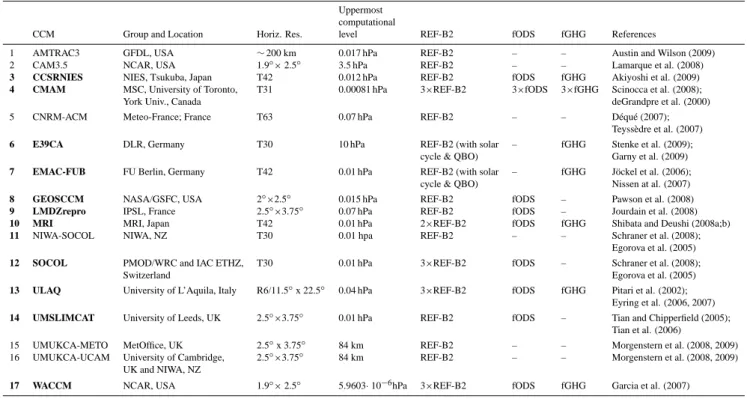
Table 1. A summary of the CCMs and simulations used in this study. REF-B2 is the future reference simulation, fODS is a simulation with
fixed ODSs and fGHG a simulation with fixed GHGs. Further details on the models can be found in Morgenstern et al. (2010) and SPARC CCMVal (2010) as well as in the references given below. CCMs that contributed sensitivity simulations are highlighted in bold. N × REF-B2 means that the group provided N realizations of this simulation. T42 approximately corresponds to 2.8◦×2.8◦, T30 to 3.75◦×3.75◦.
Uppermost computational
CCM Group and Location Horiz. Res. level REF-B2 fODS fGHG References
1 AMTRAC3 GFDL, USA ∼200 km 0.017 hPa REF-B2 – – Austin and Wilson (2009) 2 CAM3.5 NCAR, USA 1.9◦
×2.5◦ 3.5 hPa REF-B2 – – Lamarque et al. (2008)
3 CCSRNIES NIES, Tsukuba, Japan T42 0.012 hPa REF-B2 fODS fGHG Akiyoshi et al. (2009)
4 CMAM MSC, University of Toronto, T31 0.00081 hPa 3×REF-B2 3×fODS 3×fGHG Scinocca et al. (2008); York Univ., Canada deGrandpre et al. (2000) 5 CNRM-ACM Meteo-France; France T63 0.07 hPa REF-B2 – – D´equ´e (2007);
Teyss`edre et al. (2007)
6 E39CA DLR, Germany T30 10 hPa REF-B2 (with solar – fGHG Stenke et al. (2009); cycle & QBO) Garny et al. (2009)
7 EMAC-FUB FU Berlin, Germany T42 0.01 hPa REF-B2 (with solar – fGHG J¨ockel et al. (2006); cycle & QBO) Nissen at al. (2007)
8 GEOSCCM NASA/GSFC, USA 2◦×2.5◦ 0.015 hPa REF-B2 fODS – Pawson et al. (2008)
9 LMDZrepro IPSL, France 2.5◦×3.75◦ 0.07 hPa REF-B2 fODS – Jourdain et al. (2008)
10 MRI MRI, Japan T42 0.01 hPa 2×REF-B2 fODS fGHG Shibata and Deushi (2008a;b)
11 NIWA-SOCOL NIWA, NZ T30 0.01 hpa REF-B2 – – Schraner et al. (2008); Egorova et al. (2005)
12 SOCOL PMOD/WRC and IAC ETHZ, T30 0.01 hPa 3×REF-B2 fODS – Schraner et al. (2008); Switzerland Egorova et al. (2005)
13 ULAQ University of L’Aquila, Italy R6/11.5◦x 22.5◦ 0.04 hPa 3×REF-B2 fODS fGHG Pitari et al. (2002);
Eyring et al. (2006, 2007)
14 UMSLIMCAT University of Leeds, UK 2.5◦×3.75◦ 0.01 hPa REF-B2 fODS – Tian and Chipperfield (2005); Tian et al. (2006)
15 UMUKCA-METO MetOffice, UK 2.5◦x 3.75◦ 84 km REF-B2 – – Morgenstern et al. (2008, 2009)
16 UMUKCA-UCAM University of Cambridge, 2.5◦×3.75◦ 84 km REF-B2 – – Morgenstern et al. (2008, 2009)
UK and NIWA, NZ
17 WACCM NCAR, USA 1.9◦
×2.5◦ 5.9603· 10−6hPa 3×REF-B2 fODS fGHG Garcia et al. (2007)
– fGHG is a transient simulation from 1960 to 2100,
sim-ilar to REF-B2, but with GHGs fixed at 1960 levels throughout the simulation. To be consistent with the GHG evolution, SSTs and SICs are prescribed with the 1955–1964 average of the values used in REF-B2. Whether or not the chemical effects of CH4and N2O
on ozone were also fixed at 1960 levels varied between the different modeling groups (see Table 2). The inten-tion of the fGHG simulainten-tion was that the ODSs (in par-ticular the CFCs) should also not contribute to radiative forcing. However, in a number of CCMs it was only the radiative forcing for CO2, CH4and N2O that was held
constant at 1960 values. The simulation is designed to assess the impact of climate change on ozone through the 21st century. By comparing the sum of fGHG and fODS (each relative to the 1960 baseline) with REF-B2, the linear additivity of the responses can be assessed. This sensitivity simulation is identical to the SCN-B2c simulation defined in Eyring et al. (2008).
3 Analysis method for multi-model time series
The same time series additive model (TSAM) as used in Chapter 9 of SPARC CCMVal (2010) and described further
in Scinocca et al. (2010) is used here to calculate multi-model trends and their confidence and prediction uncertain-ties. Here, the term ’trend’ does not denote the result of a lin-ear regression analysis but rather it refers to a smooth trajec-tory passing through the model time series representing the “signal” resulting from forced changes and leaving ‘noise’ as a residual resulting from internal unforced climate vari-ability. The advantages of the TSAM approach are the pro-duction of smooth trend estimates out to the ends of the time series, the ability to model explicitly inter-annual variabil-ity about the trend estimate, and the abilvariabil-ity to make rigorous probability statements (Scinocca et al., 2010).
The TSAM method consists of three different steps: (i) nonparametric estimation of the individual model trends (IMT), where the time series is additively modelled as the sum of a smooth unknown model-dependent trend and ir-regular normally-distributed noise which represents natural variability about the trend; (ii) baseline adjustment of these individual model trends so that they equal zero in the refer-ence year (here 1960 or 1980); (iii) average of the baseline-adjusted IMT estimates over all models resulting in a multi-model trend (MMT) estimate for each simulation. Both the IMT and MMT estimates pass through zero at the specified reference year.
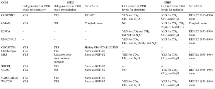
Table 2. Specifics of the sensitivity simulations with fixed ODSs (fODS) and fixed GHGs (fGHG).
CCM fODS fGHG
Halogens fixed at 1960 Halogens fixed at 1960 SSTs/SICs GHGs fixed at 1960 GHGs fixed at 1960 SSTs/SICs
levels for chemistry levels for radiation levels for chemistry levels for radiation
CCSRNIES YES YES REF-B2 YES for CO2, YES for CO2, REF-B2 1955–1964
CH4, and N2O CH4, and N2O mean
CMAM YES NO Coupled ocean NO YES for CO2, CH4, Coupled ocean
N2O, F11, and F12
E39CA – – – YES for CO2and CH4, YES for CO2, REF-B2 1955–1964
but NO for N2O CH4, and N2O mean
EMAC-FUB – – – YES for CO2, YES for CO2, REF-B2 1955–1964
CH4, and N2OCH4, and N2O mean
GEOSCCM YES YES Hadley Obs/NCAR CCSM3 – – –
LMDZrepro YES YES Same as REF-B2 – – –
MRI YES Radiation code Same as REF-B2 YES for CO2, YES for CO2, REF-B2 1955–1964
does not treat CH4, and N2O CH4, and N2O mean
halogens
SOCOL YES YES Same as REF-B2 – – –
ULAQ YES NO Same as REF-B2 NO YES for CO2, REF-B2 1955–1964
CH4, and N2O mean
UMSLIMCAT YES YES Same as REF-B2 – – –
WACCM YES YES Same as REF-B2 YES for CO2, YES for CO2, REF-B2 1955–1964
CH4, and N2O CH4, and N2O mean
Two types of uncertainty intervals are constructed for the MMT estimate. The first is the point-wise 95% confidence interval. This interval has a 95% chance of overlapping the true trend representing the local uncertainty in the trend at each year. The second interval is the 95% prediction interval which, by construction, is larger than the confidence interval. This interval is a combination of uncertainty in the trend es-timate and uncertainty due to natural inter-annual variability about the trend and gives a sense of where an ozone value for a given year might reasonably lie.
Some CCMs submitted more than one reference simula-tion (CMAM, MRI, SOCOL, ULAQ, and WACCM). In such cases the nonparametric regression is applied to the raw time series from all ensemble members to calculate a single IMT which then contributes to the multi-model mean.
To illustrate the TSAM technique, the individual IMT and MMT estimates of the global total column ozone anomaly time series for the 17 reference simulations (REF-B2) are shown in Fig. 1 (similar figures for individual regions are shown in Figs. S1 and S2 in the supplementary online ma-terial). While the 1980 return date (red vertical lines) is the same in both panels, the uncertainty (blue vertical lines) in return dates derived from the 1960 baseline adjusted column ozone anomalies is slightly larger (by up to 3 years). A sum-mary of the dates when total column ozone returns to its 1980 values, calculated from the two different time series, is given in Table 3. For consistency with the analysis presented in WMO (2007), 1980 ozone return dates in the reference sim-ulations (Sect. 5) were calculated from the 1980-baseline ad-justed time series. However, when using the fixed ODS and fixed GHG simulations to disentangle the effects of changes in climate and ODSs on ozone (Sect. 4) and to calculate dates
of full recovery of ozone from the effects of ODSs (Sect. 5), the 1960-baseline adjusted time series are used since ODSs and GHGs are fixed at 1960 values and thus the ozone time series are already quite different from the REF-B2 simula-tions by 1980.
4 Long-term ozone evolution and attribution to
different forcings
To attribute long-term changes in ozone to GHGs and ODSs, in this Section the evolution of ozone in the reference sim-ulations (REF-B2) is compared to the fixed ODS (fODS) and to the fixed GHG (fGHG) simulations. The evolution from 1960 to 2100 is assessed in the context of the 1960 baseline-adjusted ozone, temperature, transformed Eulerian mean vertical velocity (w*), and total column ozone time se-ries (Figs. 2, 3, 5, 6, 8, and 9). In addition ozone and to-tal column ozone are plotted against equivalent stratospheric chlorine (ESC, Figs. 4 and 7) using the absolute values rather than anomalies. The figures in the main paper show the 1960-baseline adjusted multi-model trend estimates for the refer-ence and sensitivity simulations, while the individual model trend estimates are shown in the figures in the supplementary online material (Figs. S3–13). The absolute values for each model in various regions and altitudes are shown in Fig. S14 to S38 in the supplementary online material. The analysis focuses on ozone in the upper (5 hPa) and lower stratosphere (50 hPa) as well as on total column ozone. The 5 and 50 hPa levels are representative for the upper and lower stratosphere, respectively. They are chosen because of the difference between chemical and dynamical control and because pre-vious studies have shown that the ozone evolution differs
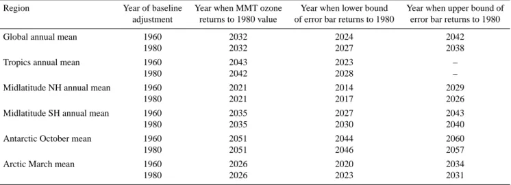
Table 3. Date of return to 1980 total column ozone in the reference simulations as derived from Fig. 10.
Region Year of baseline Year when MMT ozone Year when lower bound Year when upper bound of
adjustment returns to 1980 value of error bar returns to 1980 error bar returns to 1980
Global annual mean 1960 2032 2024 2042
1980 2032 2027 2038
Tropics annual mean 1960 2043 2023 –
1980 2042 2028 –
Midlatitude NH annual mean 1960 2021 2014 2029
1980 2021 2017 2026
Midlatitude SH annual mean 1960 2035 2027 2043
1980 2035 2030 2040
Antarctic October mean 1960 2051 2044 2060
1980 2051 2046 2057
Arctic March mean 1960 2026 2020 2034
1980 2026 2023 2031
significantly between the upper and lower stratosphere, with mostly little change in between (e.g., Eyring et al., 2007).
4.1 Tropical ozone
In the tropical upper stratosphere, all REF-B2 simulations indicate decreasing annual mean ozone between 1960 and 2000 followed by a steady increase until the end of the 21st century, while in the tropical lower stratosphere continuous ozone decreases from 1960 to 2100 are simulated in all mod-els (black line and grey shaded area in Fig. 2a and b; see also Chapter 9 of SPARC CCMVal, 2010; Austin et al., 2010 and Oman et al., 2010b).
4.1.1 Tropical upper stratospheric ozone
The elevated ozone in the tropical upper stratosphere at 5 hPa after 2000 (Fig. 2a) results from a continuous cooling caused by increasing GHGs, in particular CO2 (Clough and
Ia-cono, 1995). This continuous cooling is simulated in the multi-model trend estimate of REF-B2 (Fig. 3a) and slows gas-phase ozone loss cycles, thereby increasing ozone (e.g., Haigh and Pyle, 1982; Rosenfield et al., 2002; Jonsson et al., 2004). The cooling is very similar in the fODS simulation, whereas in the fGHG simulation temperature stay nearly con-stant over the simulated period because GHGs are fixed at 1960 levels and SSTs/SICs are forced to represent 1960 con-ditions (Fig. 3a). Consistently, the multi-model ozone trend of the fGHG simulation in the tropical upper stratosphere in Fig. 2a does not show the increase above 1980 values that is simulated in REF-B2, confirming that the CCMs are able to simulate the mechanism invoked above. In contrast, in the fODS simulation, a steady increase in tropical upper stratospheric ozone is simulated over the entire 1960 to 2100 period. At the end of the 21st century, upper stratospheric
ozone in the fGHG simulation is significantly lower than in the REF-B2 simulation, which in turn is only slightly smaller than in the fODS simulation (Fig. 2a).
The model time series plotted in Figs. 2 and 3 can be pre-sented in an alternative format by plotting ozone as a func-tion of ESC rather than time. This provides a different view on how past and future ozone changes respond to the pri-mary driver of interest, i.e. changes in stratospheric halogen loading. An attribution of ozone changes in the tropical up-per stratosphere to changes in ODSs and GHGs is displayed in this alternative format in Fig. 4a. The multi-model mean shown in this panel is calculated from the CCSRNIES, MRI, and WACCM models. CMAM was excluded from this multi-model mean since the CMAM fGHG simulation included the transient chemical effects of CH4and N2O which cause the
2000 to 2100 fGHG trace to lie below the 1960 to 2000 trace in contrast to the other models used in the multi-model mean which show close concurrence between the 1960–2000 and 2000–2100 segments of the fGHG plot (see Figs. S14 to S18 in supplementary online material). Furthermore, ULAQ was excluded from this multi-model mean since it too showed be-havior quite different to the other four models, including dis-agreement between the 1960–2000 and 2000–2100 segments in the fGHG simulation (see figures in the supplementary on-line material).
The multi-model mean REF-B2 simulation in Fig. 4a shows that ozone decreases from 1960 to 2000 in the up-per stratosphere in response to increasing ESC. However, as ESC decreases from 2000 to 2100 ozone does not simply re-trace the 1960–2000 path but shows systematically elevated ozone through the 21st century such that ozone returns to 1980 values in the late 2020s well before ESC returns to its 1980 value in the mid-2050s. As discussed above, the elevated ozone through the 21st century results from CO2
-Fig. 1. (a) 1960 and (b) 1980 baseline-adjusted annual mean global
total ozone column from the 17 reference simulations (REF-B2). The thick black line shows the multi-model mean and the light- and dark-grey shaded regions show the 95% confidence and 95% pre-diction intervals, respectively. The red vertical dashed line indicates the year when the multi-model mean returns to 1980 values and the blue vertical dashed lines indicate the uncertainty in these return dates. The green horizontal dashed line refers to the 1980 baseline, which may differ from zero when referenced to another year, e.g. 1960 as in panel (a).
induced stratospheric cooling, shown by the red to blue tran-sition from 1960 to 2100 in the REF-B2 trace in Fig. 4a. The fixed ODS simulation shows ozone in the upper strato-sphere slowly increasing with time under the influence of in-creasing CO2and resultant stratospheric cooling. In contrast
to the REF-B2 simulation, the fixed GHG simulation shows that the response of ozone to ESC through the 21st century is almost identical to that through the 20th century. In this simulation, because GHGs are fixed, temperature shows al-most no trend from 1960 to 2100 (see also Fig. 3a). To test whether the perturbations to ozone from ODS and GHG changes are independent, the ozone changes due to the com-bined effect of ODSs and GHGs changes in REF-B2 are compared to the sum of the ozone changes due to only the effect of ODSs (fGHG) and due to only effects of GHGs (fODS). The comparison is then used to test whether these two effects on ozone are linearly additive, i.e. whether the effect of ODSs (or GHGs) on ozone depends on GHG (or
ODS) levels. The close agreement between the REF-B2 and grey traces in Fig. 4a indicates that the system is close to be-ing linearly additive. The system deviates most from linear additivity in 2000 when the ozone depletion is largest. How-ever, this deviation may result from the fODS simulation be-ing forced by SSTs taken from a model simulation where the radiative forcing effects of transiently changing ODSs were included. As a result, even though the radiative effects of ODSs are kept fixed in the fODS simulation, their effects are felt to a lesser extent through the SSTs.
4.1.2 Tropical lower stratospheric ozone
In the tropical lower stratosphere, a robust feature simulated by all CCMs is that ozone in the REF-B2 simulations shows steadily declining values from 1960 to 2100 and ozone never returns to its 1980 value (Fig. 2b). The primary mecha-nism causing this trend is the increase in tropical upwelling through the 21st century, which is a robust result in CCM simulations (see Fig. 5 as well as Butchart et al. , 2006, 2010; Oman et al., 2010b; Chapter 4 of SPARC CCMVal, 2010). Tropical lower stratospheric ozone content is mostly determined by a balance between the rate of ozone produc-tion (i.e. from photolysis of O2)and the rate at which the air
is transported through and out of the tropical lower strato-sphere (Avallone and Prather, 1996). A faster transit of air through the tropical lower stratosphere from enhanced tropi-cal upwelling leads to less time for production of ozone and hence to lower ozone levels in this region. The increase in tropical upwelling in fODS is similar to that in REF-B2 in all models and in the multi-model trend, confirming that chang-ing halogens do not contribute to this trend which is caused by climate change and in particular climate-change induced SST changes. This is also evidenced by the increase in up-welling in a SOCOL fGHG simulation in which GHGs were fixed but SSTs evolved as in REF-B2 (not shown), in agree-ment with previous findings (Fomichev et al., 2007; Deckert and Dameris, 2008a, b; Oman et al., 2009). Correspond-ingly, the fGHG multi-model ozone trend in the tropical lower stratosphere (50 hPa) stays nearly constant throughout the 21st century, whereas the fODS multi-model ozone trend is very similar to that in REF-B2 and does not respond to ESC changes (red curve in Fig. 2b), indicating that this re-gion is mainly controlled by changes in climate rather than ODSs.
This is a consistent result which is simulated by nearly all models (see Figs. S3 and S4). Only ULAQ has a higher sensitivity of ozone to halogens than all other models (see also Fig. 4 of Oman et al., 2010b) which could explain why in this simulation the suppressed tropical ozone, unlike in all other models, is mainly determined by halogen changes until 2030. This is concluded from the fact that ozone in the fGHG simulation in ULAQ is nearly identical to REF-B2 until 2030 (Fig. S4b). Only after 2030 does climate change dominate halogen sensitivity in ULAQ. One reason for this
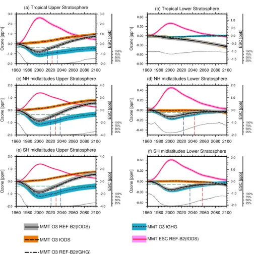
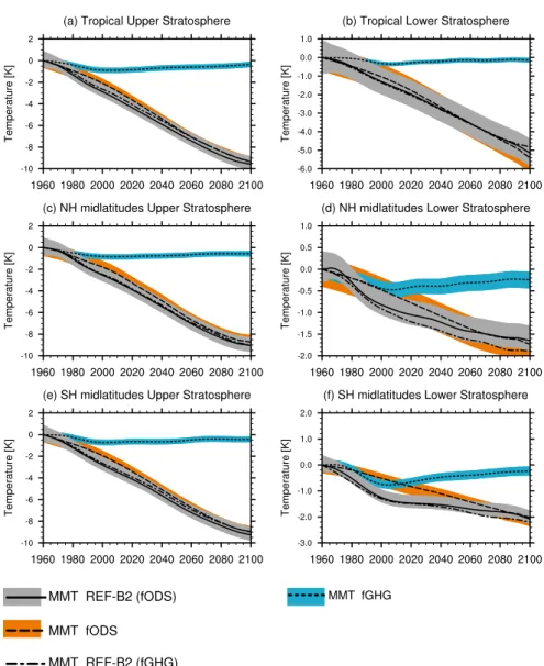
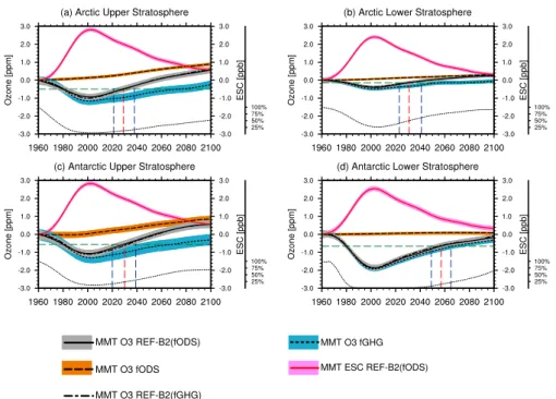
Fig. 2. Extra-polar, annual mean 1960 baseline-adjusted ozone projections and 95% confidence interval for the multi-model trend (MMT)
of REF-B2 which is derived from the models that performed the fODS simulation (MMT O3 REF-B2(fODS); black line and grey shaded area) and from the models that performed the fGHG simulation (MMT O3 REF-B2(fGHG); black dashed-dotted line). Also shown is the multi-model trend plus 95% confidence interval for fODS (black dotted line and orange shaded area), fGHG (black dashed line and blue shaded area), and ESC (MMT ESC REF-B2(fODS) displayed with red solid line and light red shaded area). The different panels show (a) 5 hPa and (b) 50 hPa tropics (25◦S–25◦N), (c) 5 hPa and (d) 50 hPa northern midlatitudes (35◦N–60◦N), (e) 5 hPa and (f) 50 hPa southern midlatitudes (35◦S–60◦S). The multi-model mean for REF-B2, fODS, and ESC is formed from 9 CCMs (CCSRNIES, CMAM, GEOSCCM, LMDZrepro, MRI, SOCOL, UMSLIMCAT, ULAQ, and WACCM) and the one for fGHG from 7 CCMs (CCSRNIES, CMAM, EMAC-FUB, E39CA, MRI, ULAQ, and WACCM). The red vertical dashed line indicates the year when the multi-model mean of the 9 CCMs in REF-B2 returns to 1980 values (green horizontal dashed line) and the blue vertical dashed lines indicate the uncertainty in these return dates. The thin dotted black line in the bottom of each panel shows the results of the t-test’s confidence level that the multi-model means from fODS and REF-B2 are from the same population (see Sect. 5 for details).The individual models are shown in figures in the supplementary material. Note the differing Y-axis scales.
could be the coarse horizontal resolution in ULAQ or that the model includes an explicit code for NAT and ice parti-cle formation, growth and transport which can form not only in the winter polar regions but also in the tropical UTLS. In addition, ULAQ includes a parameterization for upper tro-pospheric cirrus ice particles (K¨archer and Lohmann, 2002). Decreases in ozone in the lower stratosphere and total col-umn ozone in the 2nd half of the 21st century in the REF-B2 simulations of SOCOL are significantly larger than in all other simulations (Figs. S3b and S12b) due to a particularly large Brewer-Dobson circulation strength and trend (Oman et al., 2010b). For total column ozone this is similar in the other
ECHAM5 based models (EMAC-FUB and NIWA-SOCOL, see Fig. S1b).
An attribution of ozone changes in the tropical lower stratosphere to changes in ODSs and GHGs is shown in Fig. 4b. In this panel the multi-model mean was calculated using the CCSRNIES, CMAM, MRI and WACCM models (see individual models in Figs. S14 to S18 in the supple-mentary material). ULAQ was also excluded for the reasons outlined above (see also supplementary online material). In the lower stratosphere in the tropics ozone shows little re-sponse to ESC through the 20th and 21st centuries as seen from the fGHG trace. The ∼25% decrease in ozone from
Fig. 3. Same as Fig. 2, but for temperature.
1960 to 2100 in the reference scenario results from GHG-induced changes to stratospheric dynamics as evidenced by the fixed ODS scenario. Note also that in the fODS simula-tion ESC decreases with time in response to these circulasimula-tion changes. As in the upper stratosphere, the response of ozone to ODSs and GHGs is almost linearly additive as shown by the close agreement between the REF-B2 and grey traces in Fig. 4b. This indicates that ozone in the tropical lower strato-sphere responds primarily to the underlying SSTs with only a small contribution from the in situ effects of GHG radiative forcing.
4.1.3 Tropical total column ozone
The evolution of tropical column ozone (Fig. 6b) depends on the balance between the increase in upper stratospheric concentrations and the decrease in lower stratospheric
con-centrations, and as a result the projected changes are in gen-eral small compared to extra-tropical regions in the REF-B2 simulation (∼7 DU, see Table 4). In the MMT calculated from the 17 CCMs’ reference simulations, there is a gen-eral decline from the start of the integrations until the turn of the century, followed by a gradual increase until about 2050 with 70% of the simulated ozone lost since 1980 recovered by 2025 and 110% by 2050 in the multi-model mean (Ta-ble 4). After 2050, column ozone amounts decline slightly again toward the end of the century. Increased tropical up-welling is one of the largest drivers of this (see Fig. 5 as well as Shepherd, 2008 and Li et al., 2009). This is also confirmed by the similarity of the REF-B2 and fODS simu-lations in Fig. 6b after 2050. In the fGHG simulation, up-per stratospheric tropical ozone is consistently lower than in REF-B2 (Fig. 2a) while tropical upwelling is not increasing (Fig. 5), and lower stratospheric tropical ozone is higher than
0.6 0.9 1.2 1.5 1.8 2.1 2.4 2.7 3 3.3 3.6 3.9 ESC at 5hPa (ppb) 7.5 8 8.5 9 9.5 10 10.5 Oz on e( pp m) 2020 2050 2080 1960 1970 1980 1990 2000 2010 2020 2030 2040 2050 2060 2070 2080 2090 2100 -1.5 -1 -0.5 0 0.5 1 oz on ew .r.t .1 96 0( pp m) 0.4 0.5 0.6 0.7 0.8 0.9 1 1.1 1.2 1.3 1.4 ESC at 50 hPa (ppb) 1.351.4 1.451.5 1.551.6 1.651.7 1.751.8 Oz on e( pp m) 2020 2050 2080 1960 1970 1980 1990 2000 2010 2020 2030 2040 2050 2060 2070 2080 2090 2100 -0.4 -0.35 -0.3 -0.25 -0.2 -0.15 -0.1 -0.05 0 oz on ew .r.t .1 96 0( pp m) 0.4 0.5 0.6 0.7 0.8 0.9 1 1.1 1.2 1.3 1.4 ESC at 50 hPa (ppb) 255 258 261 264 267 270 273 276 To tal co lum no zo ne (D U) 2020 2050 2080 1960 1970 1980 1990 2000 2010 2020 2030 2040 2050 2060 2070 2080 2090 2100 Reference simulation Fixed ODS simulation Fixed GHG simulation
Linear additivity test -15
-12 -9 -6 -3 0 3 oz on ew .r.t .1 96 0( DU ) 5 hPa 50 hPa Column ozone Temperature Temperature 23 3. 3K 24 2. 9K 20 2. 7K 20 8. 0K REF simulation fODS simulation
Linear additivity test fGHG simulation
fODS simulation REF simulation
fGHG simulation
Linear additivity test ESC returns to
1980 values Ozone returns to 1980 values
(a)
(b)
(c)
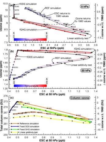
Fig. 4. (a) Annual multi-model mean tropical ozone as a
function of ESC=Cly+5×Bry at 5 hPa and averaged between 25◦S and 25◦N. (b) as in panel (a) but at 50 hPa and where ESC=Cly+60×Bry. In panels (a) and (b) the REF-B2, fODS, and fGHG simulations are shown using traces colored according to the multi-model-mean temperature using the scale shown in the bottom left of each panel. The grey traces in these two panels show the additive effects of the fODS and fGHG simulations calculated from: GreyESC(t )=fGHGESC(t )+fODSESC(t )−fODSESC(1960) and Greyozone(t ) =fGHGozone(t )+fODSozone(t )−fODSozone (1960). Differences between the grey and REF-B2 traces indicate a lack of linear additivity in the system. Panel (c), as in (b) but for total column ozone and without color coding by tempera-ture. In this panel the fODS+fGHG trace is shown in yellow (yellow=blue+green). In all three panels, on each trace, reference years are shown every 10th data point with year labels shown for the REF-B2 simulation. The multi-model means displayed in this figure were derived from a subset of the 5 models that provided both fGHG and fODS simulations (see text for details).
in REF-B2 and remains nearly constant in the fGHG simu-lation (Fig. 2b). Consistently, the MMT of tropical column ozone in fGHG is higher than REF-B2 at the end of the 21st century and returns to its 1980 values around 2060 (Fig. 6b). A comparison of the REF-B2, fODS and fGHG simula-tions for tropical total column ozone is also shown, using a different format, in Fig. 4c with the multi-model mean cal-culated from CCSRNIES, CMAM, MRI, and WACCM.
In-Fig. 5. Multi-model mean and 95% confidence interval of the 1960 baseline-adjusted annual mean w* between 20◦S and 20◦N at 70 hPa for REF-B2 (solid black line and grey shaded area) and fGHG (black dashed line and blue shaded area). The individual models are shown in the supplementary material in Fig. S11.
terestingly, unlike ozone at 5 and 50 hPa in the tropics, total column ozone shows deviations away from linear additivity demonstrated by the lack of coincidence of the orange and yellow traces in Fig. 4c. While the exact causes of such devi-ations in linear additivity are not yet known, it is possible that the inclusion of the effects of ODS radiative forcing via the SSTs used as boundary conditions in the fODS simulation may be a contributing factor.
4.2 Midlatitude ozone
4.2.1 Midlatitude upper stratospheric ozone
In the midlatitude upper stratosphere, which is mainly photo-chemically controlled, ozone increases due to CO2-induced
cooling of the stratosphere that slows chemical destruction rates. Increases in N2O and CH4 appear to play a minor
role in upper stratospheric ozone depletion under the SRES A1B GHG scenario (Eyring et al., 2007, 2010; Oman et al., 2010a).
Overall, the projected evolution of midlatitude upper stratospheric ozone is very similar to that in the tropics. In the SRES A1B GHG scenario the ozone evolution is charac-terized by increases throughout the 21st century (Fig. 2c, e) due to CO2-induced cooling (Fig. 3c, e).
4.2.2 Midlatitude lower stratospheric ozone
In the lower stratosphere the evolution of midlatitude ozone differs from that in the tropics (compare panel b in Fig. 2 with panels d and f), and rather than a steady decrease in ozone, first a decrease is simulated between 1960 and 2000, which is then followed by a steady increase throughout the 21st cen-tury. As in the tropics, changes in transport also play a role in the ozone evolution in midlatitudes but here the increase in the meridional circulation is more likely to lead to an in-crease rather than a dein-crease in ozone. Inter-hemispheric
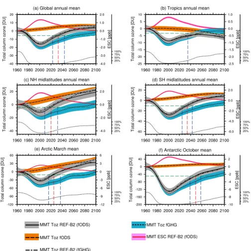
Fig. 6. 1960 baseline-adjusted total column ozone projections and 95% confidence interval for the multi-model REF-B2 trend which is in
the one case derived from the models that performed the fODS simulation (MMT O3 REF-B2(fODS); black line and grey shaded area) and in the other case from the models that performed the fGHG simulation (MMT O3 REF-B2(fGHG); black dashed-dotted line). Also shown is the multi-model trend plus 95% confidence interval for fODS (black dotted line and orange shaded area), fGHG (black dashed line and blue shaded area), and ESC (MMT ESC REF-B2(fODS; red solid line and light red shaded area). The different panels show (a) global (90◦S–90◦N annual mean), (b) tropics (25◦S–25◦N annual mean), (c) NH midlatitudes (35◦N–60◦N annual mean), (d) SH midlatitudes (35◦S–60◦S annual mean), (e) Arctic (60◦N–90◦N March mean), and (f) Antarctic (60◦S–90◦S October mean). The red vertical dashed line indicates the year when the multi-model mean in REF-B2 returns to 1980 values (green horizontal dashed line) and the blue vertical dashed lines indicate the uncertainty in these return dates. The thin dotted black line shows the results of the t-test’s confidence level that the multi-model means from fODS and REF-B2 are from the same population (see Sect. 5 for details). The individual models are shown in the supplementary material. Note the differing Y-axis scales.
differences in changes in transport could explain the hemi-spheric difference in ozone evolution, since the increase in stratospheric circulation transports more ozone into the northern midlatitudes lower stratosphere than into the SH (Shepherd, 2008; Li et al., 2009) and since in the SH the mix-ing of ozone poor air from the ozone hole into midlatitudes could also contribute. Effects of inclusion of ozone depleted over Antarctica, resulting from excursions of the Antarctic polar vortex away from the pole, in the calculation of the southern midlatitude (60◦S–35◦S) mean ozone likely also contribute to the hemispheric differences in ozone evolution.
Differences between the ozone evolution in the fGHG and REF-B2 simulations in the midlatitude lower stratosphere are generally small in both hemispheres (Fig. 2d, f), indicating that changes in GHG do not play a large role in this region. However, due to changes in transport discussed above, in REF-B2 ozone in the lower stratosphere returns to 1980 lev-els around 15 years earlier in the northern than in the south-ern midlatitudes. The temperature evolution in the midlati-tude lower stratosphere is similar to that in the tropics (com-pare panel b in Fig. 3 with panels d and f), though the tem-perature responds more to changes in ODSs through ODS induced changes in ozone (concluded by the larger differ-ence of fODS and REF-B2 in the midlatitudes), in particular
in the southern midlatitudes, consistent with previous studies (WMO, 2007; Shepherd and Jonsson, 2008).
4.2.3 Midlatitude total column ozone
Because ozone averaged over midlatitudes first decreases un-til around 2000 and then increases again in the upper and lower stratosphere over the 21st century, a similar evolution is projected for midlatitude total column ozone (Fig. 6c, d). In both hemispheres the 1960 baseline-adjusted midlatitude multi-model mean ozone indicates that the ozone minimum is reached by ∼2000 followed by a steady and significant increase. By 2025, Northern (Southern) Hemisphere col-umn ozone is projected to have regained 130% (70%) of the amount lost between 1980 and 2000 (2002) with 230% (145%) of the loss regained by 2050 (see Table 4). By 2050, midlatitude total column ozone in both hemispheres is pro-jected to be above 1980 levels, but the return to historical values in the northern midlatitudes is more advanced than in the southern midlatitudes, caused by differences in return dates in the lower stratosphere (see Fig. 2d, f), probably be-cause of strengthened transport. By 2100, the column ozone in the northern (southern) midlatitudes is projected to have increased by 22 (19) DU compared to 1980 amounts. Other influences such as NOxand HOxcatalysed ozone destruction
have small impacts because the source molecules (N2O and
H2O) have small trends in the reference simulation which is
based on the SRES A1B GHG scenario (Chapter 6 of SPARC CCMVal, 2010; Oman et al., 2010a). This is different in other GHG scenarios (see further discussion in Oman et al., 2010a and Eyring et al., 2010). In both hemispheres the total column ozone MMT in the fGHG simulation is lower than in REF-B2 (Fig. 6c, d) due to differences between these sim-ulations mainly in the upper stratosphere (Fig. 2c, e) where the GHG-induced effect on ozone is ∼10 times larger than in the lower stratosphere, where differences are very small.
An attribution of total column ozone changes in the north-ern and southnorth-ern midlatitudes to changes in ODSs and GHGs is shown in panels (b) and (c) of Fig. 7 with the multi-model mean calculated from all the 5 CCMs that performed both simulations (CCSRNIES, CMAM, MRI, ULAQ, and WACCM). The REF-B2 simulation shows that total column ozone decreases from 1960 to 2000 but at a greater rate over southern midlatitudes than over northern midlatitudes; over northern midlatitudes ozone shows a −7 DU/ppb sensitivity to ESC over the 1960 to 2000 period while over southern midlatitudes the sensitivity is −16 DU/ppb. This greater than a factor of two difference in sensitivity of southern midlati-tude ozone to ESC, and the slightly greater levels of ESC reached over southern midlatitudes, results in a 3.6% to-tal column ozone reduction over northern midlatitudes from 1960 to 2000 and an 7.7% total column ozone reduction over southern midlatitudes over this period. In both hemispheres, as ESC decreases, total column ozone does not simply re-trace the 1960–2000 path, but shows systematically elevated
400 420 440 460 480 1960 1970 1980 1990 2000 2010 2020 2030 2040 2050 2060 2070 2080 2090 2100 330 340 350 360 370 380 19601970 1980 1990 2000 2010 2020 2030 2040 2050 2060 2070 2080 2090 2100 310 320 330 340 350 360 370 19601970 1980 1990 2000 2010 2020 2030 2040 2050 2060 2070 2080 2090 2100 0.8 1 1.2 1.4 1.6 1.8 2 2.2 2.4 2.6 2.8 3 3.2 3.4 3.6 3.8 ESC (ppb) 200 220 240 260 280 300 320 340 360 1960 1970 1980 1990 2000 2010 2020 2030 2040 2050 2060 2070 2080 2090 2100 Reference simulation Fixed ODS simulation Fixed GHG simulation Linear additivity test
(a)Arctic (60oN to 90oN) (b)NH mid-latitudes (35oN to 60oN) (c)SH mid-latitudes (35oS to 60oS) (d)Antarctic (60oS to 90oS) To tal co lum no zo ne (D U) 1980 1990 2000 2030 2060 2090
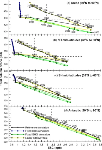
Fig. 7. As in Fig. 4, but for total column ozone in the
midlati-tudes (annual average) and polar regions (March mean in Arctic and October mean in Antarctic). The multi-model mean is calcu-lated from all models that performed both fODS and fGHG simula-tions in addition to REF-B2 i.e. CCSRNIES, CMAM, MRI, ULAQ and WACCM. ESC is shown for 50 hPa. Blue traces show results from simulations where prescribed ODSs are fixed at 1960 val-ues (fODSs). Green traces show results from simulations where prescribed GHGs are fixed at 1960 values (fGHG). Yellow traces show the additive effects of the fODS and fGHG simulations calculated from: Yellow ESC(t) = fGHGESC(t) + fODSESC(t ) – fODSESC(1960) and Yellow Ozone(t) = fGHGozone(t) + fODSozone(t ) − fODSozone (1960). Differences between the yel-low and REF-B2 traces indicate a lack of linear additivity in the system.
ozone through the 21st century. As a result, over northern midlatitudes total column ozone returns to 1980 values in the early 2020s, well before ESC returns to its 1980 value in the late 2040s. Similarly, over southern midlatitudes total col-umn ozone returns to 1980 values in the mid-2030s (a decade later than in the Northern Hemisphere), and well before ESC returns to its 1980 value in the late 2040s. It is clear from the fODS scenario (blue traces in Fig. 7), that the elevated ozone through the 21st century results from GHG-induced
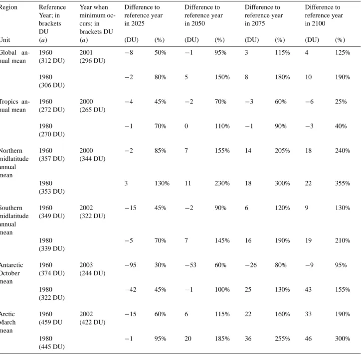
Table 4. Summary of the extent to which ozone has returned to 1960 and 1980 levels from its absolute minimum, expressed as percentages
calculated from the 1980 baseline-adjusted timeseries of all 17 CCMs’ reference simulations. 0% denotes that ozone has not increased above the minimum, 50% denotes that ozone at this date is halfway between the minimum observed and the 1960 or 1980 level, 100% denotes that ozone has returned to the 1960 or 1980 level, and >100% denotes that ozone exceeds the 1960 or 1980 level at this date.
Region Reference Year; in brackets DU Year when minimum oc-curs; in brackets DU Difference to reference year in 2025 Difference to reference year in 2050 Difference to reference year in 2075 Difference to reference year in 2100
Unit (a) (a) (DU) (%) (DU) (%) (DU) (%) (DU) (%)
Global an-nual mean 1960 (312 DU) 2001 (296 DU) −8 50% −1 95% 3 115% 4 125% 1980 (306 DU) −2 80% 5 150% 8 180% 10 190% Tropics an-nual mean 1960 (272 DU) 2000 (265 DU) −4 45% −2 70% −3 60% −6 25% 1980 (270 DU) −1 70% 0 110% −1 90% −3 40% Northern midlatitude annual mean 1960 (357 DU) 2000 (344 DU) −2 85% 7 155% 14 205% 18 240% 1980 (353 DU) 3 130% 11 230% 18 300% 22 355% Southern midlatitude annual mean 1960 (349 DU) 2002 (322 DU) −15 45% −2 90% 6 120% 9 130% 1980 (339 DU) −5 70% 7 145% 16 190% 19 210% Antarctic October mean 1960 (374 DU) 2003 (244 DU) −95 30% −53 60% −26 80% −9 95% 1980 (322 DU) −42 45% −1 100% 25 130% 43 155% Arctic March mean 1960 (459 DU 2002 (422 DU) −15 60% 6 115% 22 160% 33 190% 1980 (445 DU) −1 95% 20 185% 36 255% 46 300%
stratospheric cooling and changes in circulation. The fODS simulation also shows ESC decreasing with time even though ODSs are fixed at 1960 values. This results from the increas-ing strength of the Brewer-Dobson circulation through the 21st century and a resultant decrease in the time available to photolyze ODSs in the upper stratosphere and mesosphere. It is also clear from the REF-B2 and fODS traces in Fig. 7 that
by 2100 total column ozone over midlatitudes is still being influenced by ESC. In both the northern and southern mid-latitudes the effects of ODSs and GHGs on column ozone are approximately linearly additive (agreement of black and yellow traces in Fig. 7b and c).
Fig. 8. Same as Fig. 2, but ozone in polar regions in the Arctic (March mean, upper row) and in the Antarctic (October mean, lower row).
The upper stratosphere is shown for the 5 hPa level and the lower stratosphere for the 50 hPa level.
4.3 Polar ozone in spring
4.3.1 Antartic spring-time ozone
In the Antarctic (60◦–90◦S) in spring, the general character-istics of the ozone evolution in the CCMVal-2 reference sim-ulations are similar in all CCMs and similar to the CCM pro-jections shown in Eyring et al. (2007). Lower stratospheric ozone (Fig. 8d) and total column ozone (Fig. 6f) are domi-nated by responses to ODSs, resulting in peak ozone deple-tion around 2000 (∼80 DU lower than its 1980 value, see Table 4), followed by a slow and steady increase until 2100. By the year 2025, 45% of the ozone loss since 1980 is pro-jected to rebuild, and 100% by 2050. By the end of the 21st century, Antarctic spring ozone will have higher concentra-tions than in 1980 (+43 DU, 155%), but still be lower than in 1960 (−9 DU, 95%). The dominant role of ODSs in affecting Antarctic spring ozone is well known (Eyring et al., 2007; Chapter 9 of SPARC CCMVal, 2010) and is further con-firmed here by the large difference between the fODS simula-tion and the REF-B2 simulasimula-tion (Figs. 8d and 6f) compared to the relatively small difference between the REF-B2 and the fGHG simulations. However, climate change also plays a role in the Antarctic, and while the multi-model total col-umn ozone trend estimate for the fGHG simulation returns to 1980 values around the time when ESC does (compare dotted black line and red line in Fig. 6f), the MMT of REF-B2 re-turns earlier to 1980 levels by around 10 years (2045–2060) resulting primarily from upper stratospheric cooling (Fig. 9c) and resultant increases in ozone (Fig. 8c).
Attribution of Antarctic column ozone changes to ODSs and GHGs is shown in Fig. 7d with the multi-model mean calculated as for midlatitude total column ozone (see indi-vidual models in Figs. S34 to S38 in the supplementary ma-terial). The reference simulation shows total column ozone decreasing from 1960 to 2000 with a 52 DU/ppb sensitivity to ESC, leading to a 35% decrease in total column ozone over this period. Unlike the midlatitudes and Arctic (Fig. 7a–c), the total column ozone evolution over Antarctica (Fig. 7d) shows small sensitivity to changes in GHGs with the return path (21st century) closely tracking the outbound path (20th century). Since ozone shows only small response to GHGs in this region, assessing the additivity of the simulations is not appropriate.
4.3.2 Arctic spring-time ozone
In the Arctic (60◦–90◦N) in spring, lower stratospheric ozone (Fig. 8b) and total column ozone (Fig. 6e) follow a similar evolution to spring-time Antarctic ozone, but with smaller ozone losses during the peak ozone depletion period (∼23 DU smaller than its 1980 value, see Table 4) and with ozone increasing significantly above 1980 and even 1960 values at the end of the century in the reference simula-tion. Most of the simulations using the fixed ODS scenarios show a steady increase in Arctic ozone over the 21st century, likely related to the increases in the strength of the Brewer-Dobson circulation and enhanced stratospheric cooling as-sociated with increases in CO2. In the fixed GHG
Fig. 9. Same as Fig. 8, but for temperature.
REF-B2 (Fig. 6e), with a much later date of return of ozone column amounts to 1980 values when the counterbalancing effects of GHGs are excluded.
The attribution of Arctic ozone changes to GHG and ODS changes is further illustrated in Fig. 7a, where an attribution of total column ozone changes over the Arctic to changes in ODSs and GHGs is shown for the multi-model mean cal-culated as for midlatitude total column ozone (see individ-ual models in Figs. S29 to S33 in the supplementary ma-terial). The reference simulation shows total column ozone decreasing from 1960 to 2000 with a −14 DU/ppb sensitivity to ESC, less than the −16 DU/ppb sensitivity observed over southern midlatitudes. The increase in ESC from 1.1 ppb in 1960 to 3.5 ppb in 2000 leads to a 8.0% decrease in total col-umn ozone over this period. As for the midlatitudes, total column ozone over the Arctic is elevated above what would be expected from changes in ESC by stratospheric cooling and changes to the Brewer-Dobson circulation induced by increasing GHGs – see fixed ODS simulation. Through the latter half of the century the system shows a high degree of linear additivity (close agreement of black and yellow traces in Fig. 7a). As discussed in Butchart et al. (2010) and Chap-ter 4 of SPARC CCMVal (2010), in the models the extra ra-diative cooling from growing amounts of GHGs is approxi-mately balanced by a concomitant increase in the adiabatic
warming through increased polar downwelling with the net effect being a near zero temperature trend in the Arctic win-ter lower stratosphere. A small trend (−1 K from 2000 to 2100) is simulated in the extended set of CCMVal-2 models in March (Fig. 9b). However, it is also important to note that there is a very large spread between the fODS simulations, with some models simulating a slight increase in tempera-ture in the Arctic by 2100 (Fig. S10 in supplementary ma-terial). The large spread in the impact of GHG changes on Arctic temperature is likely to be related to changes in dy-namical heating of the Arctic linked to GHG changes. Pre-vious studies using stratospheric climate models have shown that the response to GHG changes can be very different be-tween models with different horizontal resolution (Bell et al., 2010) and that these changes are related to changes in Arc-tic dynamical heating. The impact of ozone depletion and recovery on Arctic temperatures can be diagnosed from the fGHG runs in Fig. 9a. Arctic temperatures are close to their 1960 values by 2100 in this simulation and the temperatures from fODS and fGHG appear to be additive.
5 Ozone return dates and full ozone recovery
Two distinct milestones in the future evolution of ozone, namely the return of ozone to historical values and the full
recovery of ozone from the effects of ODSs (WMO, 2007) are assessed and compared in the reference simulations (see also Introduction). Ozone return dates to 1980 values are derived from the 1960 and 1980 baseline-adjusted reference simulation (REF-B2) ozone time series. The selection of baseline adjustment has little effect on 1980 return dates and the uncertainty on that date increases by at most 3 years when shifting from 1980 to 1960 baseline adjusted time series (see Figs. 1, S1 and S2 for illustration as well as Table 3). The robustness of the 1980 return date to baseline adjustment se-lection means that 1980 ozone return dates calculated from the 1980 baseline-adjusted time series can be directly com-pared to the date of full ozone recovery which must be cal-culated from the 1960 baseline-adjusted time series. This is necessary because full recovery of ozone from the effects of ODSs is evaluated as when ozone is no longer significantly affected by ODSs (WMO, 2007), i.e. as the fODS and REF-B2 simulations converge.
Here, we apply the student’s t-test to test whether the multi-model means calculated from the fODS and REF-B2 simulations are from the same population, and use this to quantify the likelihood that full recovery has occurred. The sample variance σ2for REF-B2 and fODS in the t-test is ob-tained from the TSAM 95% prediction interval I , following the relation σ2=(I SQRT(n)/2 × 1.96)2, where n is the num-ber of models in the multi-model mean. The outcome of the t-tests is discussed using the terminology of the IPCC (see Box TS.1 of Solomon et al., 2007) to indicate the assessed likelihood: if the confidence level from the t-test is >95%, then it is extremely likely that full ozone recovery has oc-curred (within 2σ confidence), if it is >90% it is very likely that it has occurred, while if it is >66% it is likely that it has occurred (within 1σ confidence). For values between 33% and 66% probability it is about as likely as not and for values <33% it is unlikely that full recovery of ozone has occurred. Figure 10 shows the date of return to 1960 (upper panel) and 1980 (lower panel) total column ozone compared to the return date of Clyat 50 hPa and ESC at 50 hPa for the annual
average (global, tropical and midlatitude) and spring (polar) total ozone column derived from the MMT (large triangles) of the CCMVal-2 reference simulations (17 CCMs) in each latitude band. Note that the return dates differ slightly from return dates derived from the MMT in Fig. 6 where in the multi-model mean only a subset of the 17 CCMs are con-sidered. They also differ from Chapter 9 of SPARC CCM-Val (2010) that used only 16 out of the 17 CCMs used here. The MMT ESC at 50 hPa is calculated as Cly+ 60×Bry
ex-cept for one model (E39CA) where Clyinstead of ESC was
used. This model does not have available separate informa-tion about Bry, since it applies a bromine parameterisation
(see Appendix of Stenke et al., 2009).
There is no consensus between CCMs on whether tropi-cal total column ozone will return to 1980 values, with some models showing ozone increasing slightly above 1980 values by the second half of the 21st century and others with ozone
Fig. 10. Date of return to 1960 (upper panel) and 1980 (lower panel)
total column ozone (black triangle and error bar), Clyat 50 hPa (red triangle and error bar) and ESC at 50 hPa (blue triangle and error bar) for the annual average (global, tropical and midlatitude) and spring (polar) total column ozone derived from the 1980 baseline-adjusted CCMVal-2 reference simulations (17 CCMs) in each lat-itude band. The error bar shows the uncertainty in return dates as calculated from the 95% confidence interval. ESC is calculated as Cly+ 60×Bryexcept for E39CA (see text). While a few models project a return of tropical total column ozone to 1980 levels, most do not with the result that the 95% TSAM confidence interval ex-tends from 2030 to beyond the end of the century which explains the large error bar in the tropical column ozone return dates in the lower panel.
remaining below 1980 values through the 21st century (see Austin et al., 2010; Chapter 9 of SPARC CCMVal, 2010). This is reflected by the large error bar derived from the 95% TSAM confidence interval which extends from around 2030 to beyond the end of the century. However, unlike in studies mentioned above which included 16 out of the 17 CCM REF-B2 simulations used here, the addition of one model (EMAC-FUB) in this study, a model which returns to 1980 values ear-lier than the MMT in the tropics, causes the MMT to return to its 1980 value in 2041. Note also that tropical column ozone derived from the subset of 9 CCMs in Fig. 6b does also not return to its 1980 value, showing again that the tropical ozone return date is not a robust quantity across the CCMs. How-ever, there is a consensus in all CCMs that tropical column ozone will not return to 1960 values, i.e. even when
strato-spheric halogens return to historical (1960) values tropical column ozone will remain below its historical values due to the increase in tropical upwelling (see Fig. 10a and Chap-ter 9 of SPARC CCMVal, 2010). In contrast, Clyand ESC
in the tropical region return to 1980 values faster than in all other regions (Fig. 10b) with only minor difference between them. By the end of the century, it is likely (∼82%) that full recovery of tropical column ozone from the effects of ODSs will have occurred, while the 1σ confidence level (66%) is projected to be reached already ∼2074 (see Table 5). Col-umn ozone in the tropics is projected to decrease again in the 2nd half of the 21st century due to climate change (see Sect. 4.1). In the upper tropical stratosphere, ozone returns to 1980 values at ∼2020 which is faster than in other regions (see Fig. 2a), while it is about as likely as not (∼42%) that full ozone recovery has occurred by the end of the 21st cen-tury (see Table 5). In the lower tropical stratosphere however, ozone never returns to its 1980 values. That said, because ozone in this region is little affected by ODSs, the recovery of ozone from ODS effects is identified above the 1σ con-fidence level (66%) throughout the entire 21st century, and above the 2σ confidence level (95%) from 2040 onwards.
In the northern midlatitudes, total column ozone returns to 1980 values around 2021 (within a bounded range of 2017 to 2026, see Fig. 10b and Table 3). This is the earliest return in all regions considered here, in agreement with previous stud-ies (e.g., Shepherd, 2008; Austin et al., 2010; Chapter 9 of SPARC CCMVal, 2010). While the qualitative evolution is the same in both hemispheres in the CCMs, the midlatitude anomalies are larger in the SH and the return of midlatitude column ozone to 1980 values therefore occurs later in the SH (∼2035 within a bounded range of 2030 to 2040) than in the NH. The difference in the date of return to 1980 values appears to be due to inter-hemispheric difference in changes in transport, see discussion in Sect. 4.2. In all CCMs the return of total column ozone to 1980 values in the midlat-itudes occurs before that of Cly and ESC (∼2050 in both
hemispheres). In contrast, in the northern midlatitudes it is likely (71%) that full recovery of total column ozone has oc-curred by the end of the 21st century, while it is about as likely as not (61%) in the southern midlatitudes (Fig. 6c, d and Table 5). In both hemispheres, midlatitude column ozone also returns to 1960 values, but significantly later than when it returns to 1980 values (∼2055 in SH and ∼2030 in NH). In the midlatitude upper stratosphere, ozone returns to 1980 values ∼2030 (see Fig. 2c, e), while in both hemispheres full recovery of ozone from ODSs in this region of the at-mosphere is projected to not likely have occurred by 2100 (see Table 5). In the midlatitude lower stratosphere, ozone returns to its 1980 values ∼2055, while full ozone recovery at the 1σ confidence interval is reached ∼2042 in the NH and ∼2073 in the SH. By the end of the century, full ozone recovery is projected to have likely occurred in the north-ern and southnorth-ern midlatitude lower stratosphere (∼85% and 82%, respectively).
As discussed in Sect. 4.3, Antarctic spring ozone column evolution is dominated by ODSs, and in this region ozone return dates are very similar to Cly and ESC return dates
and occur later than in all other regions. Column ozone is therefore projected to return to its 1980 values around 2051 (within a bounded range of 2046 to 2057, see Table 3 and Fig. 10b). There is however a spread in the magnitude of the changes among the CCMs which can also be seen by the 95% confidence interval of the MMT (Fig. 6f) and by the un-certainty in the time of return to 1980 values. This spread is closely linked to the spread in simulated Cly(Chapter 9
of SPARC CCMVal, 2010). On the other hand, it is about as likely as not (62%) that full ozone recovery in the refer-ence simulations has occurred by the end of the 21st century (compare fODS with REF-B2 in Fig. 6f, see also Table 5), and column ozone has also not returned to its 1960 values by then (Fig. 10a).
In contrast, in the Arctic, total column ozone is projected to return to its 1980 values already around 2026 (within a bounded range of 2023 to 2031), which is much earlier than when Clyand ESC return to 1980 values in this region, and
it is also projected to return to its 1960 values (∼2041). Full recovery of total column ozone at the 1σ confidence level (66%) in the Arctic is reached earlier than in all other re-gions (∼2038) and it is likely that ozone has fully recov-ered (∼84%) by the end of the century (Fig. 6e and Table 5). Global total column ozone returns to its 1980 values around 2032 (within a bounded range of 2027 to 2038), which is earlier than global Clyor ESC at 50 hPa (Fig. 10b), while it
is about as likely as not (54%) that full ozone recovery has occurred by the end of the century (Fig. 6a).
Overall, total column ozone returns to its 1980 values in all regions, with largest uncertainty in the ozone return date estimate in the tropics, while by 2100 it returns to its 1960 values only in the midlatitudes and in the Arctic, but not over Antarctica and not in the tropics. Full recovery of ozone is projected to not likely have occurred by the end of the cen-tury in any of the upper stratosphere regions. In the tropi-cal lower stratosphere (50 hPa), however, it is projected to be very likely that full ozone recovery from ODSs has occurred by the end of the 21st century while it is likely that it occurred also over midlatitudes. For total column ozone, full ozone re-covery is not reached at the 2σ confidence level in any of the regions, while at the 1σ level it is projected to occur ∼2038 in the Arctic, ∼2070 at northern midlatitudes, and ∼2074 in the tropics, but not in the southern midlatitudes and not over Antarctica. In the southern midlatitudes and in the Antarctic it is still not likely that ozone has fully recovered from ODSs by the end of the century (61% and 62%, respectively). The larger set of models used here confirms the overall findings of Waugh et al. (2009) who assessed ozone recovery within GEOSCCM.