HAL Id: hal-00295649
https://hal.archives-ouvertes.fr/hal-00295649
Submitted on 22 Mar 2005
HAL is a multi-disciplinary open access
archive for the deposit and dissemination of
sci-entific research documents, whether they are
pub-lished or not. The documents may come from
teaching and research institutions in France or
abroad, or from public or private research centers.
L’archive ouverte pluridisciplinaire HAL, est
destinée au dépôt et à la diffusion de documents
scientifiques de niveau recherche, publiés ou non,
émanant des établissements d’enseignement et de
recherche français ou étrangers, des laboratoires
publics ou privés.
emissions of Scots pine
V. Tarvainen, H. Hakola, H. Hellén, J. Bäck, P. Hari, M. Kulmala
To cite this version:
V. Tarvainen, H. Hakola, H. Hellén, J. Bäck, P. Hari, et al.. Temperature and light dependence of
the VOC emissions of Scots pine. Atmospheric Chemistry and Physics, European Geosciences Union,
2005, 5 (4), pp.989-998. �hal-00295649�
Atmos. Chem. Phys., 5, 989–998, 2005 www.atmos-chem-phys.org/acp/5/989/ SRef-ID: 1680-7324/acp/2005-5-989 European Geosciences Union
Atmospheric
Chemistry
and Physics
Temperature and light dependence of the VOC emissions of Scots
pine
V. Tarvainen1, H. Hakola1, H. Hell´en1, J. B¨ack2, P. Hari2, and M. Kulmala3
1Finnish Meteorological Institute, Sahaajankatu 20 E, FI-00880 Helsinki, Finland 2Department of Forest Ecology, University of Helsinki, Helsinki, Finland 3Department of Physical Sciences, University of Helsinki, Helsinki, Finland
Received: 10 August 2004 – Published in Atmos. Chem. Phys. Discuss.: 19 October 2004 Revised: 1 March 2005 – Accepted: 3 March 2005 – Published: 22 March 2005
Abstract. The volatile organic compound (VOC) emission
rates of Scots pine (Pinus sylvestris L.) were measured from trees growing in a natural forest environment at two locations in Finland. The observed total VOC emission rates varied be-tween 21 and 874 ng g−1h−1and 268 and 1670 ng g−1h−1in southern and northern Finland, respectively. A clear seasonal cycle was detected with high emission rates in early spring, a decrease of the emissions in late spring and early summer, high emissions again in late summer, and a gradual decrease in autumn.
The main emitted compounds were 13-carene (southern Finland) and α- and β-pinene (northern Finland), with ap-proximate relative contributions of 60–70% and 60–85% of the total observed monoterpene emission rates, respectively. Sesquiterpene (β-caryophyllene) and 2-methyl-3-buten-2-ol (MBO) emissions were initiated in early summer at both sites. The observed MBO emission rates were between 1 and 3.5% of the total monoterpene emission rates. The sesquiter-pene emission rates varied between 2 and 5% of the total monoterpene emission rates in southern Finland, but were high (40%) in northern Finland in spring.
Most of the measured emission rates were found to be well described by the temperature dependent emission algo-rithm. The calculated standard emission potentials were high in spring and early summer, decreased somewhat in late sum-mer, and were high again towards autumn. The experimen-tal coefficient β ranged from 0.025 to 0.19 (average 0.10) in southern Finland, with strongest temperature dependence in spring and weakest in late summer. Only the emission rates of 1,8-cineole were found to be both light and temperature dependent.
Correspondence to: V. Tarvainen
1 Introduction
Scots pine (Pinus sylvestris L.) is one of the most com-mon tree species in the boreal forests, and e.g. in Finland its volatile organic compound (VOC) emissions dominate the annual biogenic VOC emissions (Lindfors and Laurila, 2000; Lindfors et al., 2000). The monoterpene emission charac-teristics of Scots pine have been described in several stud-ies (Janson, 1993; Rinne et al., 1999, 2000; Staudt et al., 2000; Janson et al., 2001; Komenda and Koppmann, 2002). Janson and de Serves (2001) have also measured high ace-tone emission rates from Scots pine. So far sesquiterpenes have not been detected in the emissions of Scots pine al-though other boreal tree species, such as Norway spruce (Picea abies L.) and Downy birch (Betula pubescens L.) emit large amounts of sesquiterpenes during summer (Hakola et al., 2000, 2003). 2-methyl-3-buten-2-ol (MBO) has been ob-served to be a main component in the air in a pine forest in Colorado (Goldan et al., 1993). Harley et al. (1998) have also measured high MBO emission rates from the needles of several pine species but it has not previously been reported in the emissions of Scots pine in boreal forests.
Once emitted, both sesquiterpenes and MBO are very re-active, the sesquiterpenes especially so, with an atmospheric lifetime of only a few minutes so that they can not be mea-sured in ambient air samples (Hakola et al., 2000, 2003). In daytime, the main sink of MBO is assumed to be the reac-tion with OH radicals but it also reacts with ozone and ni-trate radical, producing acetone, aldehydes, formic acid, and organic, carbonyl and peroxy nitrates (Finlayson-Pitts and Pitts, 2000, and references therein) thus affecting local pho-tochemistry and atmospheric ozone formation. Sesquiter-penes react readily with atmospheric ozone, and they have a high potential to form secondary organic aerosol (Hoffmann et al., 1997; Jaoui et al., 2003). Bonn and Moortgat (2003) suggest that sesquiterpene ozonolysis could be involved in the atmospheric new particle formation observed frequently
in several locations including Hyyti¨al¨a, Finland (M¨akel¨a et al., 1997; Boy and Kulmala, 2002). The new particle for-mation and growth processes are, however, probably uncou-pled (Kulmala et al., 2000), and the oxidation products of the sesquiterpenes are expected to mainly affect the growth of the particles (see, e.g. Kulmala et al., 2004). Sesquiter-penes also affect tropospheric ozone concentrations, by par-ticipating in ozone formation when enough nitrogen oxides are present or acting as ozone sink in a very clean environ-ment, where some of the ozone deposition may be attributed to sesquiterpene reactions (Kurpius and Goldstein, 2003). Currently, the sesquiterpene emission rate data of boreal tree species is very limited.
We have measured the VOC emission rates of Scots pine in two locations in Finland. The seasonal development of the emissions was studied over a period of six months. Also the sesquiterpene and MBO emission rates were measured. The light and temperature dependence of the emissions was stud-ied by darkening experiments and by fitting the experimen-tal data to the light and/or temperature dependent emission algorithms commonly used in biogenic emission modelling (Guenther et al., 1993; Guenther, 1997).
2 Materials and methods
2.1 Emission measurements
The VOC emission rates of Scots pine (Pinus sylvestris L.) were measured in southern Finland in Hyyti¨al¨a (61◦510N,
24◦170E) and in the Finnish Lapland in Sodankyl¨a (67◦220N,
26◦390E). In Hyyti¨al¨a the measurements were carried out
from March to October in 2003. During the QUEST II (Quantification of Aerosol Nucleation in the European Boundary Layer) campaign (24 March to 14 May 2003) the emission rates were measured daily around noon. Sev-eral samples were usually taken per measurement session at 30 min to 2 h intervals. During three intensive campaign days the measurements were conducted during the whole day. Af-ter the campaign the emission rates were measured during 1– 2 days every month until October 2003. We also conducted experiments where the plant was covered from light.
In Hyyti¨al¨a the measured tree was growing in a natural forest environment, with an average tree height of 14 m. The samples were collected at a height of about 11 m. The mea-sured branch received direct sunlight only for a couple of hours in a day. Altogether 132 regular samples (no artifi-cial light conditions) were taken during the measurement pe-riod. In Sodankyl¨a the VOC emissions of Scots pine were measured in spring and early summer 2002. The measure-ments were carried out during five days, starting at the end of April and continuing until the beginning of June, with a total of 22 samples. The tree measured in Sodankyl¨a was younger than the one in Hyyti¨al¨a, with a height of about 5 m, and it was growing in a sunny forest environment. The same
branch was used for the measurements until the tree started to grow new needles, after which a different branch was sam-pled each time. In Hyyti¨al¨a the branch was placed in the cuvette when the measurements started in March and it re-mained there until May. After that the branch was placed in the cuvette in the evening and the sampling was started the following day. In Sodankyl¨a the branch was placed in the cuvette in the morning and samples were taken around noon. Even though the adaptation period in Sodankyl¨a was shorter than that in Hyyti¨al¨a, successive samples showed no decreas-ing trend in the emission rate that could have been caused by the handling of the branch.
The emission rates were measured using a dynamic flow through technique. The measured branch was enclosed in a Teflon cuvette with a volume of approximately 20 l. The cuvette was equipped with inlet and outlet ports and a ther-mometer. The photosynthetically active photon flux den-sity (PPFD) was measured just above the cuvette. Dur-ing the measurements in Hyyti¨al¨a the PPFD varied between 0 and 1800 µmol photons m−2s−1 and the temperature be-tween −5 and 32◦C, so a wide range of environmental con-ditions was covered. The flow through the cuvette was about 8 l min−1. Ozone was removed from the inlet air using a pack of MnO2-coated copper nets. The samples were collected onto adsorbent tubes simultaneously from both the inlet and outlet ports. The emission rate (E) is determined as the mass of compound per needle dry weight and time according to
E = (C2−C1)F
m . (1)
Here C2is the concentration in the outgoing air, C1 is the concentration in the inlet air, and F is the flow rate into the cuvette. The dry weight of the biomass (m) was determined by drying the needles at 75◦C until consistent weight was achieved.
The samples were collected on adsorbent tubes filled with Tenax-TA and Carbopack-B. The sampling time was 30– 120 min. The samples were stored in a refrigerator for less than a week prior to analysis in the laboratory. The adsor-bent tubes were analyzed using a thermodesorption instru-ment (Perkin-Elmer ATD-400) connected to a gas chromato-graph (HP 5890) with HP-1 column (60 m, i.d. 0.25 mm) and a mass-selective detector (HP 5972). Samples were con-centrated in the thermodesorption instrument in a cold trap (−30◦C). The analytical system did not allow the separa-tion of myrcene and β-pinene; their amount was therefore expressed as a sum and quantified as β-pinene. Quantifi-cation was achieved with five-point calibration using liquid standards in methanol solutions. Standard solutions were in-jected onto adsorbent tubes that were flushed with helium (flow 100 ml min−1) for 5 min in order to remove methanol.
The detection limit for isoprene and MBO was 32 ng m3. The detection limits of the monoterpenes were 11 ng m3for camphene, 42 ng m3for 13-carene, 84 ng m3for 1,8-cineole, 60 ng m3 for limonene, 30 ng m3 for α-pinene, 36 ng m3for
V. Tarvainen et al.: VOC emissions of Scots pine 991
β-pinene, 59 ng m3 for sabinene, 29 ng m3 for terpinolene, and 79 ng m3 for β-caryophyllene. These detection limits correspond to emission rates between 0.6 and 3.3 ng g−1h−1 for the monoterpenes and approximately 4.5 ng g−1h−1 for 1,8-cineole and β-caryophyllene. The error of the emission rate measurements was evaluated by simultaneously measur-ing two different branches of the same tree. Altogether 40 samples were taken and the measured emission rates were standardized to 303.15 K and 1000 µmol photons m−2s−1. The relative standard deviation of the emission rate measure-ment was about 40% for the monoterpenes, 50% for isoprene and MBO, and 60% for the sesquiterpenes. There were very few unresolved peaks that could be mono- or sesquiterpenes in the chromatograms, thus the likelihood of significant con-tributions from unidentified species is very small.
2.2 Emission algorithms
When modelling the biogenic VOC emissions for e.g. emis-sion inventory purposes or for local photochemistry studies, two mechanisms are generally considered: the temperature controlled volatilization of hydrocarbons from storage pools inside the leaf (Ciccioli et al., 1997; Guenther et al., 1993; Hauff et al., 1999; Lamb et al., 1985; Schuh et al., 1997), and the direct emissions of newly synthesized hydrocarbons, which are under enzymatic control and strongly dependent on leaf temperature and light intensity (e.g. Monson et al., 1995). Monoterpenes are usually described as storage pool emissions, while isoprene is thought to be emitted directly after the synthesis and not stored inside the plant. How-ever, several authors have reported both light and temperature controlled emissions of terpenoids other than isoprene from some plant species, including Sots pine (e.g. Hansen and Seufert, 2003; Shao et al., 2001; Schuh et al., 1997; Staudt et al., 1997; Steinbrecher and Hauff, 1996; Steinbrecher et al., 1999; Seufert et al., 1997; Komenda et al., 1999).
In this work we have calculated the emission potentials of Scots pine in Sodankyl¨a and Hyyti¨al¨a by fitting the experi-mental data to the temperature and light dependent emission algorithms proposed by Guenther et al. (1993) and Guen-ther (1997). The observed emission rate (E) is parameterised as
E = γ E0, (2)
where E0 is the emission rate at standard conditions (303.15 K, 1000 µmol photons m−2s−1), henceforth called the standard emission potential, and γ is a non-dimensional environmental correction factor which includes the effects of temperature and light conditions.
For pool emissions the environmental correction factor is (Guenther et al., 1993)
γP =exp(β(T − TS)) . (3)
Here T (K) is the leaf temperature and TS is the leaf
tem-perature at standard conditions. β is an empirical coefficient,
which is usually set at 0.09 (Guenther et al., 1993). In this work, however, we carried out nonlinear regression in order to fit also the β coefficient individually for each compound.
The environmental correction factor for the direct emis-sions of newly synthesized compounds is of the form
γS =CTCL, (4)
where CT is the temperature correction and CL is the light
correction. These are parameterised as (Guenther, 1997)
CL= αCL1L √ 1 + α2L2 (5) CT = exp([CT1(T − TS)]/RTST ) CT3+exp([CT2(T − TM)]/RTST ) . (6)
Here again T (K) is the temperature and TS is the standard
temperature. Lis the photosynthetically active photon flux density (PPFD, µmol photons m−2s−1), R is the universal gas constant, and CL1, CT1, CT2, CT3, TM and α are
empir-ical constants given by Guenther (1997).
3 Results and discussion
3.1 Observed emissions
In Finland Scots pine has two genotypes that differ in the emitted monoterpene composition. One genotype mainly emits 13-carene while the other does not emit 13-carene at all (Hiltunen, 1968). The trees measured in the present study turned out to be of different types. The tree growing in So-dankyl¨a emitted no 13-carene, and 60–85% of its emission consisted of α- and β-pinene and myrcene, whereas the emis-sion of the tree measured in Hyyti¨al¨a mainly consisted of
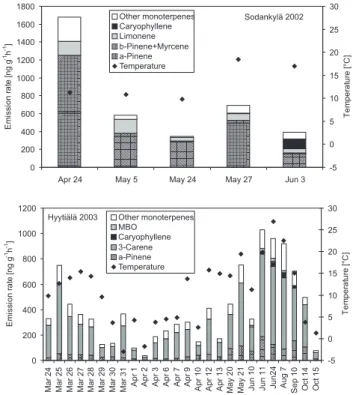
13-carene (60–70%). The average noontime emission rates observed in Sodankyl¨a and Hyyti¨al¨a during their respective measurement periods are presented in Fig. 1.
The observed total VOC emission rates were of the same order of magnitude at both locations, varying between 268 and 1670 ng g−1h−1 in Sodankyl¨a and between 21 and 874 ng g−1h−1 in Hyyti¨al¨a. The very low emissions in Hyyti¨al¨a in the beginning of April 2003 (Fig. 1, lower panel) are explained by a cold spell with temperatures close to or below zero during the two days. In general, the emissions observed in Sodankyl¨a were higher than those in Hyyti¨al¨a. In Hyyti¨al¨a, a clear seasonal cycle was detected with high emission rates in early spring, a decrease of the emissions in late spring and early summer, high emissions again in late summer, and a gradual decrease in autumn.
According to the statistics of the Finnish Meteorological Institute the weather conditions during the measurements in 2002 were exceptional, which might partly explain the high emissions observed in Sodankyl¨a. The thermal spring started earlier than normal, especially in the northern parts of the country. In addition, the spring was very warm, with
0 200 400 600 800 1000 1200 1400 1600 1800
Apr 24 May 5 May 24 May 27 Jun 3
E m is si on ra te [n g g -1h -1] -5 0 5 10 15 20 25 30 Te m per at ur e [°C ] Other monoterpenes Caryophyllene Limonene b-Pinene+Myrcene a-Pinene Temperature Sodankylä 2002 0 200 400 600 800 1000 1200 Ma r2 4 Ma r2 5 Ma r2 6 Ma r2 7 Ma r2 8 Ma r2 9 Ma r3 0 Ma r3 1 Ap r1 Ap r2 Ap r3 Ap r6 Ap r7 Ap r9 Ap r1 0 Ap r1 2 Ap r1 3 Ma y 20 Ma y 21 Ju n 10 Ju n 11 Jun24 Aug 7 Se p 10 Oc t1 4 Oc t1 5 E m is si on ra te [n g g -1h -1] -5 0 5 10 15 20 25 30 Te m per at ur e [°C ] Other monoterpenes MBO Caryophyllene 3-Carene a-Pinene Temperature Hyytiälä 2003
Fig. 1. Average noontime emission rates measured in April– June 2002 in Sodankyl¨a and in March–October 2003 in Hyyti¨al¨a. Other monoterpenes comprises camphene, sabinene, 1,8-cineole, linalool, and bornyl acetate in Sodankyl¨a, and camphene, sabinene, β-pinene+myrcene, terpinolene, limonene, 1,8-cineole,
β-phellandrene, terpinolene, and bornyl acetate in Hyyti¨al¨a. The average temperature during the measurements (solid diamonds) is shown on the right hand axis. Note that the x-axis is not in scale be-cause the averages for each measurement day are shown at regular intervals.
record high temperatures in the north, and the growing sea-son started much earlier than normal. In 2003 the spring and early summer were cooler than average in the southern parts of the country, while the temperatures were close to long term averages in August, September and October.
There were also changes in the composition of the emis-sions during the measurement period. In Sodankyl¨a, the April emissions were dominated by α- and β-pinene, with approximate relative contributions of 35% and 40% of the observed total monoterpene emission rates, respectively. In May and June the contribution of β-pinene was reduced to the 5% level, while α-pinene remained the most abundant emitted compound (55–80%) throughout the measurement period. In Hyyti¨al¨a, the contribution of α-pinene was at the 10% level in early spring, after which it doubled and stayed around 20% until October. The contribution of 13-carene, on the other hand, was approximately 70% in March and April, after which it dropped slightly, and was around 60–65% dur-ing the rest of the measurement period.
In early summer, sesquiterpene (β-caryophyllene) and 2-methyl-3-buten-2-ol (MBO) emissions were detected at both
sites, although the emission rates were very low. In So-dankyl¨a the MBO emission rates were approximately 1–2% of the total monoterpene emission rates, and in Hyyti¨al¨a, they stayed between 2–3.5% of the total monoterpene emis-sions from the onset of the emisemis-sions until the cessation in September. The observed β-caryophyllene emission rates, on the other hand, were about 40% and 2% of the observed total monoterpene emission rates in June in Sodankyl¨a and Hyyti¨al¨a, respectively. Later in summer the β-caryophyllene emissions in Hyyti¨al¨a were slightly higher, reaching approx-imately 5% of the observed total monoterpene emissions in August. The sesquiterpene emissions in Hyyti¨al¨a also ceased in September. In addition to β-caryophyllene also some other unidentified sesquiterpenes were detected. In So-dankyl¨a the other sesquiterpenes are tentatively identified as longifolene and elemene according to the NIST mass spec-tra library. These other sesquiterpenes were emitted at about the same rate as β-caryophyllene in May, but their emission rates did not increase in June like the emission rates of β-caryophyllene. Also in Hyyti¨al¨a other sesquiterpenes than
β-caryophyllene were detected, tentatively identified as α-farnesene and α-caryophyllene. However, at both sites β-caryophyllene was the dominant sesquiterpene.
3.2 Light dependence of emissions
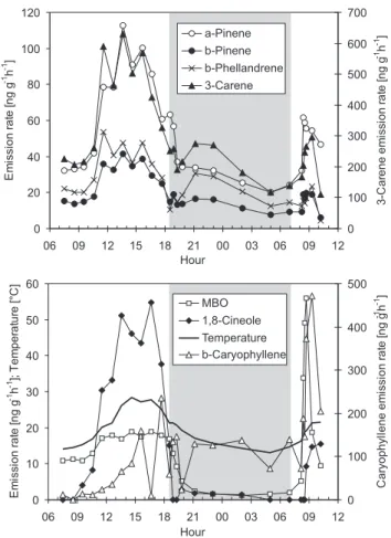
To study the light dependence of the monoterpene emissions of Scots pine we conducted experiments in which the mea-sured branch was covered from light and samples were col-lected from the darkened cuvette. The experiment presented here was started at 7 a.m. on 7 August. Hourly emission sam-ples were first collected from the selected branch under nor-mal light conditions during the day. The cuvette was covered from light at 6.30 p.m. and sampling was continued through-out the night and for several hours after the removal of the cover at 7 a.m. on 8 August.
The emissions measured during the experiment are shown in Fig. 2 together with the temperature in the cuvette. The emission rates of all monoterpenes had already decreased from the high midday values when the cuvette was darkened and after recovering from an initial drop in the emissions they continued to do so also in the complete darkness, in har-mony with the decreasing temperature (Fig. 2, upper panel, temperature in lower panel). The emissions of MBO and 1,8-cineole, however, disappeared almost completely when the cuvette was darkened, while the β-caryophyllene emis-sion rates stayed at the approximate average level of the rates measured when the cuvette was receiving light (Fig. 2, lower panel). After the cover was removed, both the MBO and β-caryophyllene emission rates rapidly increased to quite high values for a few hours before adjusting approximately to the level of the previous day. The 1,8-cineole emission rates also recovered after the cover was removed, but there was no sud-den emission burst. The MBO emissions increased immedi-ately after removing the cover, whereas the β-caryophyllene
V. Tarvainen et al.: VOC emissions of Scots pine 993
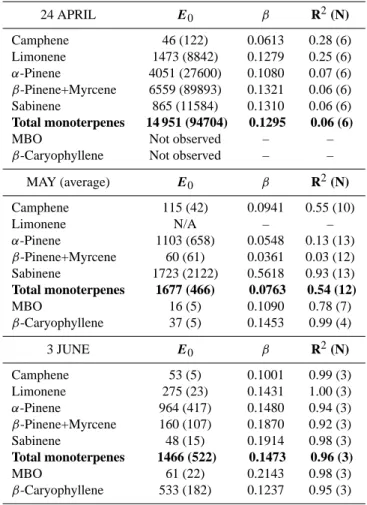
Table 1. Standardized (30◦C) seasonal emissions in Hyyti¨al¨a in 2003. The standard emission potentials E0(ng g−1h−1) and the
empirical β coefficients were obtained by a nonlinear regression fit of the data to the pool algorithm of Guenther et al. (1993) (Eq. 3). The standard error of the estimate is given in parenthesis. R squared and the number of observations (N) are also given for each case. N/A indicates that the regression either did not converge or was inconclusive. SPRING E0 β R2(N) Camphene 39 (13) 0.0926 0.47 (44) 13-Carene 1642 (850) 0.1042 0.33 (44) Limonene 13 (7) 0.0572 0.12 (36) β-Phellandrene 98 (57) 0.0707 0.16 (44) α-Pinene 196 (57) 0.0981 0.56 (44) β-Pinene 52 (25) 0.0824 0.26 (44) Sabinene 74 (36) 0.1031 0.34 (44) Terpinolene 44 (19) 0.0810 0.33 (39) Total monoterpenes 2144 (1005) 0.0994 0.35 (44)
MBO Not observed – –
β-Caryophyllene Not observed – –
EARLY SUMMER E0 β R2(N) Camphene 103 (16) 0.1167 0.66 (35) 13-Carene 4010 (556) 0.1931 0.85 (35) Limonene 33 (16) 0.1056 0.16 (27) β-Phellandrene 71 (32) 0.0907 0.26 (26) α-Pinene 677 (108) 0.1374 0.72 (35) β-Pinene 158 (24) 0.1612 0.78 (35) Sabinene 130 (22) 0.1731 0.80 (29) Terpinolene 66 (16) 0.1446 0.70 (22) Total monoterpenes 5184 (733) 0.1759 0.83 (35) MBO 92 (19) 0.1349 0.82 (12) β-Caryophyllene 160 (160) 0.1855 0.60 (4) LATE SUMMER E0 β R2(N) Camphene 37 (2) 0.0780 0.76 (29) 13-Carene 696 (56) 0.0981 0.66 (29) Limonene 14 (1) 0.0904 0.66 (21) β-Phellandrene 29 (3) 0.0248 0.08 (28) α-Pinene 130 (6) 0.0819 0.77 (29) β-Pinene 44 (2) 0.0786 0.72 (29) Sabinene 36 (3) 0.0760 0.53 (27) Terpinolene 20 (2) 0.0352 0.19 (27) Total monoterpenes 1015 (52) 0.0824 0.72 (29) MBO 28 (1) 0.0763 0.83 (24) β-Caryophyllene N/A – – AUTUMN E0 β R2(N) Camphene 135 (55) 0.1151 0.70 (21) 13-Carene 3836 (2616) 0.1483 0.61 (23) Limonene 16 (3) 0.0374 0.68 (9) β-Phellandrene N/A – – α-Pinene 869 (462) 0.1126 0.56 (23) β-Pinene 108 (50) 0.1014 0.55 (24) Sabinene 33 (18) 0.0615 0.27 (17) Terpinolene 70 (42) 0.0798 0.31 (20) Total monoterpenes 3428 (1612) 0.1074 0.58 (24) MBO N/A – – β-Caryophyllene 158 (295) 0.1606 0.16 (8)
emissions started to increase about an hour later together with the 1,8-cineole emissions.
The behaviour of the monoterpenes after the darkening of the cuvette is in agreement with that described by Niinemets and Reichstein (2003) as typical for highly volatile com-pounds whose emissions are not under stomatal control. The
Hour Hour 0 20 40 60 80 100 120 06 09 12 15 18 21 00 03 06 09 12 E m is si on ra te [n g g -1h -1] 0 100 200 300 400 500 600 700 3-C ar ene em is si on ra te [n g g -1h -1] a-Pinene b-Pinene b-Phellandrene 3-Carene 0 10 20 30 40 50 60 06 09 12 15 18 21 00 03 06 09 12 E m is si on ra te [n g g -1h -1]; Te m per at ur e [°C ] 0 100 200 300 400 500 C ar yophy llene em is si on ra te [n g g -1h -1] MBO 1,8-Cineole Temperature b-Caryophyllene
Fig. 2. Variation of the VOC emission rates of Scots pine and the
temperature in Hyyti¨al¨a during the darkening experiment on 7–8 August 2003. The branch was covered from light at 6:30 p.m. on the 7th and the cover was removed at 7:00 a.m. on the 8th.
analysis of Niinemets and Reichstein (2003) further predicts bursts of emission after stomatal opening for more water sol-uble compounds, such as MBO. The results of this experi-ment further suggest that MBO emission rates may be de-pendent on the light intensity as well as the temperature, as proposed by Harley et al. (1998). This could also be true for 1,8-cineole which showed zero emissions at the end of the darkening period.
3.3 Calculated emissions
3.3.1 Standard emission potentials
The existence of light and temperature dependencies of the measured emission rates was further studied and the standard emission potentials were calculated using emission mod-elling techniques. In this analysis the measured emission rates were fitted to both the temperature dependent pool algo-rithm (Eq. 3) and the combined light and temperature depen-dent algorithm (Eq. 4) using nonlinear regression. Since not only the emission rates but also the spectrum of the emitted
Spring 0 200 400 600 800 1000 1200 24/ 03 24/ 03 25/ 03 25/ 03 25/ 03 26/ 03 29/ 03 01/ 04 02/ 04 02/ 04 02/ 04 03/ 04 06/ 04 10/ 04 12/ 04 E m is si on ra te [n g g -1h -1] observed model Early summer 0 200 400 600 800 1000 1200 1400 20/ 05 20/ 05 20/ 05 20/ 05 20/ 05 21/ 05 21/ 05 21/ 05 21/ 05 10/ 06 10/ 06 11/ 06 11/ 06 11/ 06 11/ 06 11/ 06 11/ 06 11/ 06 E m is si on ra te [n g g -1h -1] observed model (a) Late summer 0 200 400 600 800 1000 1200 1400 24/ 06 24/ 06 24/ 06 24/ 06 24/ 06 24/ 06 07/ 08 07/ 08 07/ 08 07/ 08 07/ 08 07/ 08 08/ 08 08/ 08 08/ 08 E m is si on ra te [n g g -1h -1] observed model Autumn 0 100 200 300 400 500 600 700 800 10/ 09 10/ 09 10/ 09 10/ 09 10/ 09 14/ 10 14/ 10 14/ 10 14/ 10 15/ 10 15/ 10 15/ 10 E m is si on ra te [n g g -1h -1] observed model (b)
Fig. 3. (a) Measured and modelled 13-carene emissions in Hyyti¨al¨a in spring and early summer in 2003. Note that the x-axis is not in scale because each measurement is shown using regular intervals. The error bars indicate the 95% confidence limits of the nonlinear regression fit.
(b) Same as (a) but for late summer and autumn in 2003.
compounds showed significant variation during the measure-ment period, the data from Hyyti¨al¨a was divided into sea-sonal data sets according to the average thermal seasons. In the southern parts of Finland thermal spring (defined as the period with the smoothed daily average temperature be-tween 0 and 10◦C) usually starts in late March and lasts until early May, while thermal summer (daily average temperature above 10◦C) extends from mid-May to September, accord-ing to the statistics of the Finnish Meteorological Institute. In this analysis the summer period was further divided into early (20 May through 11 June) and late (24 June through 8 August) summer. The rest of the measurements (9 September through 15 October) were considered to represent autumn. The data from Sodankyl¨a, on the other hand, was so sparse and scattered that no seasonal grouping was possible, and thus each month was treated separately.
Most of the measured emission rates were well de-scribed by the temperature dependent pool algorithm (Eq. 3), whereas the combined temperature and light algorithm (Eq. 4) generally performed poorly in the nonlinear regres-sion analysis. The standard emisregres-sion potentials obtained by fitting the temperature algorithm to the spring, early sum-mer, late sumsum-mer, and autumn data from Hyyti¨al¨a, with the corresponding β coefficient values and the nonlinear
regres-sion statistics are given in Table 1. The standard emisregres-sion potentials obtained by fitting the temperature algorithm to the April, May and June data from Sodankyl¨a with the β coefficient values and regression statistics are given in Ta-ble 2. Only nonzero measured emission rates were included in the analysis. Also cases where the regression statistics are poor are shown in order to facilitate an evaluation of the per-formance of the algorithm during different seasons and with different compounds.
In general it can be said that for most of the modelled monoterpenes, the standardized emission potentials were high in spring and especially early summer, decreased some-what in late summer, and were high again towards autumn. This type of seasonal behaviour with higher spring emission potentials has also been observed elsewhere (Janson, 1993; Komenda and Koppmann, 2002).
In Hyyti¨al¨a the β coefficient values obtained for the differ-ent compounds ranged from 0.025 to 0.19, with an average of 0.10 (Table 1). The average value is close to the empiri-cal value 0.09 which is usually assigned to the coefficient in biogenic emission modelling studies (Guenther et al., 1993; Guenther, 1997). The highest coefficient values, indicating the strongest temperature dependence, were obtained in early summer (average 0.15), while the dependence was weakest
V. Tarvainen et al.: VOC emissions of Scots pine 995
in late summer (average 0.07). In Sodankyl¨a the coefficient values were between 0.036 and 0.56, with an average of 0.14 (Table 2).
3.3.2 Applicability of the algorithms
According to the results, the temperature algorithm was not as successful in describing the spring emissions as those dur-ing the other seasons in Hyyti¨al¨a. In Sodankyl¨a there are so few data that one should be very careful in evaluating the applicability of the algorithm based on this analysis, but also there the performance of the algorithm improves towards summer. It is quite probable, in fact, that in addition to tem-perature there are other processes during the spring recovery period of vegetation, perhaps related to the plant develop-mental stage or the environdevelop-mental conditions (e.g. strong ir-radiance in connection with rather low temperatures and low water availability), which also affect the emission patterns (B¨ack et al., in preparation, 20051).
In addition to the general tendency of poor spring per-formance, there are also differences related to the different compounds. For example in Hyyti¨al¨a limonene is extremely poorly described in spring and early summer while the algo-rithm performs reasonably well in predicting limonene emis-sions in late summer and autumn. β-phellandrene, on the other hand does not seem to be captured by the algorithm at all, and its performance with sabinene and terpinolene be-comes poorer as the summer progresses. However, these compounds are only minor constituents of the total monoter-pene emission and their emission data are therefore more un-certain, bringing an added uncertainty also to the nonlinear regression analysis.
Harley et al. (1998) have reported high emission rates of MBO from several pine species. They also found that these emissions were both temperature and light dependent, whereas in this study the MBO emissions appear to be well described by the temperature dependent pool algorithm (R2 between 0.78 and 0.98). Fitting the measured MBO data to the combined temperature and light dependent algorithm (Eq. 4) resulted in a very poor agreement (R2below 0.10). Harley et al. (1998) have pointed out that quantitative analy-sis of MBO presents several challenges. Although the stan-dard solution behaved well in the analysis, we cannot totally rule out the possibility of dehydration of MBO in real sam-ples since small amounts of isoprene were also detected.
The 1,8-cineole emissions measured in Hyyti¨al¨a in 2003, on the other hand, were well described by the light and tem-perature dependent algorithm (Eq. 4), yielding a standard emission potential of 68±4 ng g−1h−1over the whole mea-surement period (R2of 0.84; 14 observations). The pool al-gorithm (Eq. 3) performed almost equally well, with a stan-dard emission potential of 68±8 ng g−1h−1and β coefficient 1B¨ack, J., Hari, P., Hakola, H., Juurola, E., and Kulmala, M.:
Dynamics of monoterpene emissions on Pinus sylvestris during early spring, in preparation, 2005.
Table 2. Standardized (30◦C) emissions in Sodankyl¨a in 2002. The standard emission potentials E0(ng g−1h−1) and the empirical β
coefficients were obtained by a nonlinear regression fit of the data to the pool algorithm of Guenther et al. (1993) (Eq. 3). The standard error of the estimate is given in parenthesis. R squared and the num-ber of observations (N) are also given for each case. N/A indicates that the regression either did not converge or was inconclusive.
24 APRIL E0 β R2(N) Camphene 46 (122) 0.0613 0.28 (6) Limonene 1473 (8842) 0.1279 0.25 (6) α-Pinene 4051 (27600) 0.1080 0.07 (6) β-Pinene+Myrcene 6559 (89893) 0.1321 0.06 (6) Sabinene 865 (11584) 0.1310 0.06 (6) Total monoterpenes 14 951 (94704) 0.1295 0.06 (6)
MBO Not observed – –
β-Caryophyllene Not observed – –
MAY (average) E0 β R2(N) Camphene 115 (42) 0.0941 0.55 (10) Limonene N/A – – α-Pinene 1103 (658) 0.0548 0.13 (13) β-Pinene+Myrcene 60 (61) 0.0361 0.03 (12) Sabinene 1723 (2122) 0.5618 0.93 (13) Total monoterpenes 1677 (466) 0.0763 0.54 (12) MBO 16 (5) 0.1090 0.78 (7) β-Caryophyllene 37 (5) 0.1453 0.99 (4) 3 JUNE E0 β R2(N) Camphene 53 (5) 0.1001 0.99 (3) Limonene 275 (23) 0.1431 1.00 (3) α-Pinene 964 (417) 0.1480 0.94 (3) β-Pinene+Myrcene 160 (107) 0.1870 0.92 (3) Sabinene 48 (15) 0.1914 0.98 (3) Total monoterpenes 1466 (522) 0.1473 0.96 (3) MBO 61 (22) 0.2143 0.98 (3) β-Caryophyllene 533 (182) 0.1237 0.95 (3)
0.1367 (R2of 0.83). The few 1,8-cineole emission rates mea-sured in Sodankyl¨a in June 2002 were also well described by the temperature and light dependent algorithm (Eq. 4), with a standard emission potential of 246±27 ng g−1h−1(R2 of 0.80; 3 observations). The pool algorithm (Eq. 3) yielded a slightly higher emission potential 280±147 ng g−1h−1 and
β coefficient 0.1557 (R2of 0.92). Thus, the regression pro-duced almost identical results, even though in both cases the emission potentials given by the pool algorithm had larger standard deviations. However, in this analysis 1,8-cineole was the only compound with which the light and temper-ature dependent algorithm performed well, and keeping in mind the results of the darkening experiment, we may tenta-tively identify Scots pine as a light and temperature depen-dent 1,8-cineole emitter. However, our data is very limited –
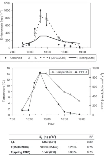
0.73 0.0674 1642 (850) T(spring 2003) 0.78 0.2614 50323 (65442) T(25.03.2003) 0.89 -6460 (571) T,L R2 b E0 [ng g h ]-1 -1 0.73 0.0674 1642 (850) T(spring 2003) 0.78 0.2614 50323 (65442) T(25.03.2003) 0.89 -6460 (571) T,L R2 b E0 0 200 400 600 800 1000 1200 7:00 10:00 13:00 16:00 19:00 E m is si on ra te [n g g -1h -1] Observed T,L T (25/03/2003) T (spring 2003) 0 2 4 6 8 10 12 14 16 7:00 10:00 13:00 16:00 19:00 Hour Te m per at ur e [°C ] 0 200 400 600 800 1000 P P FD [m m ol phot ons m -2s -1] Temperature PPFD
Fig. 4. Measured and modelled 13-carene emissions in Hyyti¨al¨a on 25 March 2003 (upper panel). The light and temperature dependent algorithm (Eq. 4) is denoted by T, L. The temperature algorithm (Eq. 3) is denoted by T. T(25/03/2003) is fitted to the data of 25 March only, while T(spring 2003) refers to the seasonally fitted al-gorithm (same as in the upper panel of Fig. 3a). The error bars indicate the 95% confidence limits of the nonlinear regression fit to T, L. The lower panel shows the temperature and the photosyn-thetically active radiation (PPFD). The standard emission potentials (30◦C) obtained with the different models are given under the fig-ure, together with the standard error of the estimate (in parenthesis), the β coefficient (when applicable) and R squared.
for example in Hyyti¨al¨a cineole was observed in only 14 of the 132 samples, and more measurements are needed, espe-cially in the late summer conditions when the emissions were highest.
In Hyyti¨al¨a, 13-carene was the main compound emitted by Scots pine throughout the study period. The observed and modelled 13-carene emissions for the spring, early and late summer and autumn measurement periods are presented in Figs. 3a and b. Even though the seasonal emissions are rather well predicted by the model based on the simple temperature algorithm (statistics in Table 1), there is some discrepancy, especially in spring. The high emissions of 25 March, in par-ticular, are not captured by the model. As pointed out above,
light dependent monoterpene emissions have been found by several authors (e.g. Hansen and Seufert, 2003; Shao et al., 2001; Schuh et al., 1997; Staudt et al., 1997; Steinbrecher and Hauff, 1996; Steinbrecher et al., 1999; Seufert et al., 1997; Komenda et al., 1999). We therefore also applied the light and temperature dependent emission model (Eq. 4) to the 13-carene data of 25 March. The results are shown in Fig. 4, together with the predictions of the average season-ally fitted temperature algorithm, and a dedicated temper-ature algorithm fitted to the data of 25 March only. The light and temperature dependent algorithm (denoted “T, L” in the figure) captures the daily emission cycle rather well (R2 of 0.89), whereas the dedicated temperature algorithm (T(25/03/2003)) underpredicts the morning and noontime emissions and overpredicts the afternoon and early evening emissions. However, the standard emission potential given by the dedicated temperature algorithm is too large to be re-alistic, and the corresponding β coefficient is also very high. The average spring algorithm (T(spring 2003)), on the other hand, is only able to produce one third of the observed daily maximum emission while also overpredicting the late after-noon emissions.
In search for an explanation for this type of sudden emis-sion bursts in spring one could argue that while monoter-penes are usually emitted from storage pools, the pools might be empty after winter, and when the plant starts to synthesize monoterpenes the emission might at first occur in concert with the light dependent production. Then as the season pro-gresses and the pools start to fill, the emission becomes sat-urated and assumes the more stable temperature dependent pattern. However, our present data is too limited to deduce the origin of this irregular emission behaviour.
Even though the emission burst of 25 March remains un-explained, these results suggest that there may be several dif-ferent processes which all contribute to the 13-carene emis-sions of Scots pine. As there were also other irregularities in the modelled monoterpene emissions when compared to the observations, such processes may apparently be active or in-active at different times during the growing season, bringing an added uncertainty to e.g. regional emission models where annual, seasonal, or other average standard emission poten-tials are used.
4 Conclusions
In conclusion we can say that a clear seasonal cycle has been established for the monoterpene emissions of Scots pine growing in a boreal forest environment. The emission rates are very high in spring, somewhat lower in early summer and high again in late summer, with a gradual decrease in autumn. The spectrum of the emitted compounds also varies during the course of the growing season; the very reactive sesquiterpenes and MBO, for instance, are emitted in quan-tity only during part of the growing season. It is obvious
V. Tarvainen et al.: VOC emissions of Scots pine 997
that these seasonal and spectral variations must be taken into consideration when constructing emission inventories to be used in e.g. atmospheric chemistry modeling in the boreal environment.
According to our results, the simple temperature depen-dent emission algorithm and seasonal emission potentials can be applied to adequately predict the emission rates of most of the compounds emitted by Scots pine. However, our re-sults also suggest that especially during the spring recovery period of the vegetation there may be several different pro-cesses contributing to the monoterpene emissions of Scots pine, and that such processes may also be active or inac-tive at other times during the growing season. Thus, further measurements, preferably combined with plant physiologi-cal data and/or modelling are needed to resolve the details of the emission processes on those occasions.
When standardized to 25◦C, the average noontime
monoterpene emission rate in our study is 1.16 µg g−1h−1, which is in accordance with earlier measurements of Scots pine. Komenda and Koppmann (2002) measured stan-dardized emission rates between 0.06–0.64 µg g−1h−1 for young pines and 0.24–3.7 µg g−1h−1for mature pines. Jan-son (1993) has also reported values quite close to our mea-surements (0.8 µg g−1h−1). The seasonal behaviour of the standard emission potential in our study, with high emission potentials in spring and early summer, lower in late summer and higher again towards autumn, is also in accordance of the seasonal behaviour observed in other similar studies (Janson, 1993; Komenda and Koppmann, 2002). The average β coef-ficient value obtained in Hyyti¨al¨a is 0.10, which is very close to the empirical value of 0.09 usually applied in biogenic emission modelling studies (Guenther et al., 1993; Guenther, 1997).
The darkened enclosure experiments did not resolve the issue of temperature and light dependence of 1,8-cineole and MBO. Based on the experiments and the nonlinear regres-sion analysis of the measured emisregres-sion rates, however, we can tentatively identify Scots pine as a light and temperature dependent 1,8-cineole emitter. The light and temperature dependence of MBO emissions found in some studies (e.g. Harley et al., 1998), on the other hand, can not be confirmed, as the light and temperature dependent algorithm failed dur-ing all seasons, while the temperature dependent algorithm captured the emission pattern fairly well in summer. In order to properly assess the dependencies and the standard emis-sion potentials of these compounds further measurements are needed, especially in late summer when the emissions are highest.
According to our results, Scots pine emits sesquiterpenes only during the summer months. Thus it is not likely that they could cause the new particle formation events observed in Hyyti¨al¨a during spring (Kulmala et al., 2001) – however, their oxidation products can participate in the growth pro-cesses of the newly formed particles later in the summer.
Edited by: A. Laaksonen
References
Bonn, B. and Moortgat, G. K.: Sesquiterpene ozonolysis: origin of atmospheric new particle formation from biogenic hydrocarbons, Geophys. Res. Lett., 30, 1585, doi:10.1029/2003GL017000, 2003.
Boy, M. and Kulmala, M.: Nucleation events in the continental boundary layer; Influence of physical and meteorological param-eters, Atmos. Chem. Phys., 2, 1–16, 2002,
SRef-ID: 1680-7324/acp/2002-2-1.
Ciccioli, P., Fabozzi, C., Brancaleoni, E., Cecinato, A., Frattoni, M., Bode, K., Torres, L., and Fugit, J.-L.: Use of isoprene al-gorithm for predicting the monoterpene emission from Mediter-ranean holm oak Quercus Ilex L: performance and limits of this approach, J. Geophys. Res., 102, 23 319–23 328, 1997.
Finlayson-Pitts, B. J. and Pitts Jr., J. N.: Chemistry of the upper and lower atmosphere, Academic Press, San Diego, California, 969, 2000.
Goldan, P. D., Kuster, W. C., and Fehsenfeld, F. C.: The observa-tion of a C5 alcohol emission in a North American pine forest, Geophys. Res. Lett., 20, 1039–1042, 1993.
Guenther, A., Zimmerman, P. R., Harley, P. C., Monson, R. K., and Fall, R.: Isoprene and monoterpene emission rate variability: Model evaluations and sensitivity analyses, J. Geophys. Res., 98, 12 609–12 617, 1993.
Guenther, A.: Seasonal and spatial variations in natural volatile or-ganic compound emissions, Ecol. Appl., 7(1), 34–45, 1997. Hakola, H., Laurila, T., Rinne, J., and Puhto, K.: The ambient
con-centrations of biogenic hydrocarbons at a Northern European, boreal site, Atmos. Environ., 34, 4971–4982, 2000.
Hakola, H., Tarvainen, V., Laurila, T., Hiltunen, V., Hell´en, H., and Keronen, P.: Seasonal variation of VOC concentrations above a boreal coniferous forest, Atmos. Environ., 37, 1623–1634, 2003. Hansen, U. and Seufert, G.: Temperature and light dependence of β-caryophyllene emission rates, J. Geophys. Res., 108(D24), 4801, doi:10.1029/2003JD003853, 2003.
Harley, P., Fridd-Stroud, V., Greenberg, J., Guenther, A., and Vas-concellos, P.: Emission of 2-methyl-3-buten-2-ol by pines: A potentially large natural source or reactive carbon to the atmo-sphere, J. Geophys. Res., 103(D19), 25 479–25 486, 1998. Hauff, K., R¨ossler, J., Hakola, H., and Steinbrecher, R.: Isoprenoid
emission in European Boreal forests, in: Proc. of EUROTRAC Symposium ’98, edited by: Borrell, P. M. and Borrell, P., WIT Press, Southampton, 97–102, 1999.
Hiltunen, R.: Genetic variation and interrelationships of the cortical monoterpenes, foliar mineral elements, and growth characteris-tics of eastern white pine, Diss., Michigan State University, USA, 1968.
Hoffmann, T., Odum, J. R., Bowman, F., Collins, D., Klockow, D., Flagan, R. C., and Seinfeld, J. H.: Formation of organic aerosols from the oxidation of biogenic hydrocarbons, J. Atmos. Chem., 26, 189–222, 1997.
Jaoui, M., Leungsakul, S., and Kamens, R. M.: Gas and particle products distribution from the reaction of β-caryophyllene with ozone, J. Atmos. Chem., 45, 261–287, 2003.
Janson, R.: Monoterpene emissions from Scots Pine and Norwegian Spruce, J. Geophys. Res., 98, 2839–2850, 1993.
Janson, R. and De Serves, C.: Acetone and monoterpene emissions from the boreal forest in northern Europe, Atmos. Environ., 35, 4629–4637, 2001.
Janson, R., Rosman, K., Karlsson, A., and Hansson, H.-C.: Bio-genic emissions and gaseous precursors to forest aerosols, Tellus B, 53, 423–440, 2001.
Komenda, M., Koppmann, R., von Czapiewski, K., and Wildt, J.: Emissions of volatile organic compounds from pines (Pi-nus sylvestris): a comparison of laboratory and field studies, P1.30, Book of Abstracts of the Sixth Scientific Conference of the International Global Atmospheric Chemistry Project (IGAC), Bologna, Italy, September 13–17, 44, 1999.
Komenda, M. and Koppmann, R.: Monoterpene
emis-sions from Scots pine (Pinus sylvestris): Field studies of emission rate variabilities, J. Geophys. Res., 107, D13, doi:10.1029/2001JD000691, 2002.
Kulmala, M., Pirjola, L., and M¨akel¨a, J. M.: Stable sulphate clusters as a source of new atmospheric particles, Nature, 404, 66–69, 2000.
Kulmala, M., H¨ameri, K., Aalto, P. P., M¨akel¨a, J. M., Pirjola, L., Nilsson, E. D., Buzorius, G., Rannik, ¨U., Dal Maso, M., Seidl, W., Hoffmann, T., Janson, R., Hansson, H. C., Viisanen, Y., Laaksonen, A., and O’Dowd, C. D.: Overview of the interna-tional project on biogenic aerosol formation in the boreal forest (BIOFOR), Tellus B, 53, 324–343, 2001.
Kulmala, M., Vehkam¨aki, H., Pet¨aj¨a, T., Dal Maso, M., Lauri, A., Kerminen, V.-M., Birmili, W., and McMurry, P. H.: Formation and growth rates of ultrafine atmospheric particles: A review of observations, J. Aerosol Sci., 35, 143–176, 2004.
Kurpius, M. R. and Goldstein, A. H.: Gas-phase chemistry domi-nates O3 loss to a forest, implying a source of aerosols and hy-droxyl radicals to the atmosphere, Geophys. Res. Lett., 30, 1371, doi:10.1029/2002GL016785, 2003.
Lamb, B., Westberg, H., Allwine, E., and Quarles, T.: Biogenic hydrocarbon emissions from deciduous and coniferous species in the US, J. Geophys. Res., 90, 2380–2390, 1985.
Lindfors, V. and Laurila, T.: Biogenic volatile organic compound (VOC) emissions from forests in Finland, Boreal Environ. Res., 5, 95–113, 2000.
Lindfors, V., Laurila, T., Hakola, H., Steinbrecher, R., and Rinne, J.: Modeling speciated terpenoid emissions from the European boreal forest, Atmos. Environ., 34, 4983–4996, 2000.
Monson, R. K., Lerdau, M. T., Sharkey, T. D., Schimel, D. S., and Fall, R.: Biological aspects of constructing volatile organic compound emission inventories, Atmos. Environ., 29(21), 2983– 3002, 1995.
M¨akel¨a, J. M., Aalto, P., Jokinen, V., Pohja, T., Nissinen, A., Palm-roth, S., Markkanen, T., Seitsonen, K., Lihavainen, H., and Kul-mala, M.: Observation of ultrafine aerosol particle formation and growth in boreal forest, Geophys. Res. Lett., 24, 1219–1222, 1997.
Niinemets, ¨U. and Reichstein, M.: Controls on the emission of plant volatiles through stomata: Different sensitivity of emission rates to stomatal closure explained, J. Geophys. Res., 108(D7), 4208, doi:10.1029/2002JD002620, 2003.
Rinne, J., Hakola, H., and Laurila, T.: Vertical fluxes of monoter-penes above a Scots pine stand in the boreal vegetation zone, Phys. Chem. Earth (B), 24, 711–715, 1999.
Rinne, J., Hakola, H., Laurila, T., and Rannik, ¨U.: Canopy scale monoterpene emissions of Pinus sylvestris dominated forests, Atmos. Environ., 34, 1099–1107, 2000.
Schuh, G., Heiden, A. C., Hoffmann, Th., Kahl, J., Rockel, P., Rudolph, J., and Wildt, J.: Emissions of volatile organic com-pounds from sunflower and beech: dependence on temperature and light intensity, J. Atmos. Chem., 27, 291–318, 1997. Seufert, G., Bartzis, J., Bomboi, T., Ciccioli, P., Cieslik, S., Dlugi,
R., Foster, P., Hewitt, C. N., Kesselmeier, J., Kotzias, D., Lenz, R., Manes, F., Perez-Pastor, R., Steinbrecher, R., Torres, L., Valentini, R., and Versino, B.: The BEMA-project: an overview of the Casterporziano experiments, Atmos. Environ., 31 (SI), 5– 18, 1997.
Shao, M., Czapiewski, K. V., Heiden, A. C., Kobel, K., Komenda, M., Koppmann, R., and Wildt, J.: Volatile organic compound emissions from Scots pine: Mechanisms and description by al-gorithms, J. Geophys. Res., 106(D17), 20 483–20 492, 2001. Staudt, M., Bertin, N., Hanse, U., Seufert, G., Ciccioli, P., Foster,
P., Frenzel, B., and Fugit, J.-L.: Seasonal and diurnal patterns of monoterpene emissions from Pinus pinea (L.) under field condi-tions, Atmos. Environ., 32, 145–156, 1997.
Staudt, M., Bertin, N., Frenzel, B., and Seufert, G.: Seasonal vari-ation in amount and composition of monoterpenes emitted by young Pinus pinea trees – Implications for emission modelling, J. Atmos. Chem., 35, 77–99, 2000.
Steinbrecher, R. and Hauff, K.: Isoprene and monoterpene emis-sion from Mediterranean oaks, in: Proc. of EUROTRAC Sym-posium ’96, edited by: Borrell, P. M., Borrell, P., Kelly, K., Cvitaˇs, T., and Seiler, W., Computational Mechanics Publica-tions, Southampton, 229–233, 1996.
Steinbrecher, R., Hauff, K., Hakola, H., and R¨ossler, J.: A revised parameterization for emission modeling of isoprenoids for Bo-real plants, in: Biogenic VOC Emissions and Photochemistry in the Boreal Regions of Europe – Biphorep, edited by: Lau-rila, T. and Lindfors, V., Air Pollution Research Report No. 70, Commission of the European Communities, Luxembourg, 29– 43, 1999.