Pattern dynamics, pattern hierarchies, and forecasting in complex multi-scale earth systems

HAL Id: hal-00298711

https://hal.archives-ouvertes.fr/hal-00298711

HAL is a multi-disciplinary open access

archive for the deposit and dissemination of sci-entific research documents, whether they are pub-lished or not. The documents may come from teaching and research institutions in France or abroad, or from public or private research centers.

L’archive ouverte pluridisciplinaire HAL, est destinée au dépôt et à la diffusion de documents scientifiques de niveau recherche, publiés ou non, émanant des établissements d’enseignement et de recherche français ou étrangers, des laboratoires publics ou privés.

Pattern dynamics, pattern hierarchies, and forecasting

in complex multi-scale earth systems

J. B. Rundle, D. L. Turcotte, P. B. Rundle, G. Yakovlev, R. Shcherbakov, A.

Donnellan, W. Klein

To cite this version:

J. B. Rundle, D. L. Turcotte, P. B. Rundle, G. Yakovlev, R. Shcherbakov, et al.. Pattern dynam-ics, pattern hierarchies, and forecasting in complex multi-scale earth systems. Hydrology and Earth System Sciences Discussions, European Geosciences Union, 2006, 3 (3), pp.1045-1069. �hal-00298711�

HESSD

Full Screen / Esc

Printer-friendly Version Interactive Discussion

EGU Hydrol. Earth Syst. Sci. Discuss., 3, 1045–1069, 2006

www.hydrol-earth-syst-sci-discuss.net/3/1045/2006/ © Author(s) 2006. This work is licensed

under a Creative Commons License.

Hydrology and Earth System Sciences Discussions

Papers published in Hydrology and Earth System Sciences Discussions are under open-access review for the journal Hydrology and Earth System Sciences

Pattern dynamics, pattern hierarchies,

and forecasting in complex multi-scale

earth systems

J. B. Rundle1,2, D. L. Turcotte3, P. B. Rundle1,2, G. Yakovlev2, R. Shcherbakov2, A. Donnellan4, and W. Klein5

1

Department of Physics, University of California, Davis, CA, USA

2

Computational Science and Engineering Center, University of California, Davis, CA, USA

3

Geology Department, University of California, Davis, CA, USA

4

Earth and Space Science Division, Jet Propulsion Laboratory, Pasadena, CA, USA

5

Department of Physics, Boston University, Boston, MA, USA

Received: 9 February 2006 – Accepted: 15 February 2006 – Published: 20 June 2006 Correspondence to: J. B. Rundle (jbrundle@ucdavis.edu)

HESSD

Full Screen / Esc

Printer-friendly Version Interactive Discussion

Abstract

Catastrophic disasters afflicting human society are often triggered by tsunamis, earth-quakes, widespread flooding, and weather and climate events. As human populations increasingly move into geographic areas affected by these earth system hazards, fore-casting the onset of these large and damaging events has become increasingly

ur-5

gent. In this paper we consider the fundamental problem of forecasting in complex multi-scale earth systems when the basic dynamical variables are either unobservable or incompletely observed. In such cases, the forecaster must rely on incompletely de-termined, but “tunable” models to interpret observable space-time patterns of events. The sequence of observable patterns constitute an apparent pattern dynamics, which

10

is related to the underlying but hidden Newtonian dynamics by a complex dimensional reduction process. As an example, we examine the problem of earthquakes, which must utilize current and past observations of observables such as seismicity and sur-face strain to produce forecasts of future activity. We show that numerical simulations of earthquake fault systems are needed in order to relate the fundamentally

unobserv-15

able nonlinear dynamics to the readily observable pattern dynamics. We also show that the space-time patterns produced by the simulations lead to a scale-invariant hierar-chy of patterns, similar to other nonlinear systems. We point out that a similar program of simulations has been very successful in weather forecasting, in which current and past observations of weather patterns are routinely extrapolated forward in time via

20

numerical simulations in order to forecast future weather patterns.

1 Introduction

The critical need to forecast natural hazards has been underscored by the 26 Decem-ber 2004 M∼9.3 Sumatra earthquake and tsunami that led to the deaths of more than 275 000 persons (Lay et al., 20051); Hurricane Katrina, a category 5 storm that

weak-25

1

HESSD

Full Screen / Esc

Printer-friendly Version Interactive Discussion

EGU ened to a category 3 storm before flooding New Orleans and the Gulf Coast of the

United States on August 29, 2005, causing as much as $130 billion in damages and killing more than 1000 persons (J. Travis, 20052); and the M∼7.6 Pakistan earthquake of 8 October 2005 with estimated fatalities of more than 87 000 persons3. Secondary disasters can also occur such as landslides, flooding, and tornadoes.

5

Given the spatial scales of these events, and the rapid onset of their most severe effects, the development of a physics-based understanding of these hazards must be a high priority, especially since human populations are increasingly moving into the areas most likely to be affected by these disasters. A physical understanding of these dynamical processes leads to the possibility of forecasting and prediction, based upon

10

the use of numerical simulations, similar to the methods by which progress has been made in the field of weather and climate forecasting during the past few decades.

Earthquakes are an example of a threshold system, in which the stress on a fault in-creases persistently due to plate tectonic forces. In general, driven nonlinear threshold systems are comprised of interacting spatial networks of statistically identical,

nonlin-15

ear units or cells that are subjected to a persistent driving force or current. A cell “fires” or “fails” when the force, electrical potential, or other physical variable σ(x, t) in a cell

at positionx and time t reaches a predefined force threshold σF. The result is an in-crease in an internal state variable s(x, t) of the cell, as well as a decrease in the force

or potential sustained by the cell to a residual value σR. Thresholds, residual stresses,

20

and internal states may be modified by the presence of quenched disorder, and the dynamics also may be modified by the presence of noise or disorder. Interactions be-tween cells may be excitatory (positive) in the sense that failure of connected neighbors brings a cell closer to firing, or inhibiting (negative) in the opposite case.

In the case of earthquake fault systems, the cell or site represents a locationx on

25

a fault; the state variable σ(x, t) represents the stress; the force threshold σF is the static frictional strength; and the residual value σR is the fault stress at the conclusion

2

http://www.nhc.noaa.gov/archive/2005/tws/MIATWSAT aug.shtml

3

HESSD

Full Screen / Esc

Printer-friendly Version Interactive Discussion of sliding. In earthquake fault systems, the fault slips when the static frictional threshold

is reached, in a process that reduces the stress to a lower, residual value. As a result of the earthquake, a portion of the stress is lost during the event, and the remainder is redistributed to other faults and regions in the system. If the redistributed stress leads to a state of supercritical stress on other faults, an avalanche of triggered failures

5

may occur, increasing the magnitude of the earthquake. Other examples of threshold systems are common in nature, and include the occurrence of floods in river networks, landslides, volcanic eruptions, ecological systems, saturation and soil moisture, and bi-ological epidemics. Threshold systems are also seen in other science and engineering applications, such as depinning transitions in charge density waves and

superconduc-10

tors, magnetized domains in ferromagnets, sandpiles, and foams (Rundle et al., 2000, 2002). As another example, for neural networks a cell is a neuron, σ(x, t) represents

the cellular electrical potential, σF is the firing potential, and σR is the potential after the cell discharges.

The failure of the levees when Hurricane Katrina struck New Orleans was also an

15

example of a threshold process. Here the large amounts of rainfall and the storm surges led to overfilling of Lake Ponchartrain and the catastrophic failure of the levee system that protected the sections of the city lying below sea level.

Both weather and seismicity are complex, chaotic phenomena. Current weather pat-terns are routinely extrapolated forward in order to forecast the weather several days

20

into the future. These forecasts utilize numerical simulations of atmospheric behavior. A specific example concerns the future tracks of hurricanes. The standard approach is to utilize ensemble forecasting. Forecasts are made using a variety of numerical simu-lations. If these simulations converge on similar tracks, then the forecast is considered robust. The question is whether a similar approach can be developed for earthquake

25

forecasting, and whether it can then be extended to other driven systems common in geomorphology and hydrology.

HESSD

Full Screen / Esc

Printer-friendly Version Interactive Discussion

EGU

2 Patterns in El Nino events

Among the fields of research that have recently made significant progress in recog-nizing, interpreting, and predicting such patterns are weather forecasting, specifically predictions in the onset of El Nino-Southern Oscillation events. These methods uti-lize variations of Principal Component Analysis, Principal Oscillation Pattern Analysis,

5

and Singular Spectrum Analysis (Preisendorfer, 1988; Penland, 1989; Penland and Sardeshmukh, 1995; Penland and Mangorian, 1993; Broomhead and King, 1986; Vau-tard and Ghil, 1989). Prediction of pattern development and evolution is complicated by the presence of noise, nonlinear mode interactions, and a variety of other factors, but progress has been made in recent years as exemplified by the successful

predic-10

tion of the El Nino weather event of 1998. In most of these methods, it is assumed that the observed time series have Markov characteristics, so that the observed state of the system at time t+∆t depends only on the observed state of the system at time t. There are typically many time scales in the dynamics, some of which can be as small as∆t, and others that can be much longer.

15

However, in making El Nino forecasts for a year in advance, it is typical to focus on processes, such as sea surface warming off the Pacific coast of South America, that take place over the preceeding weeks to months. This assumption of a relatively small range in time scale evidently holds reasonably well for El Nino events.

An additional important assumption made by some investigators is that the

space-20

time patterns of El Nino events can be considered to be described by a linear stochastic equation (Penland and Matrosova, 2006; Penland and Sardeshmukh, 1995), which is used to forecast the future occurrence and evolution of El Nino events. In this proce-dure, which we summarize briefly here, the evolution of tropical sea surface tempera-ture (SST) anomaly θ(x, t) is represented as a stable linear process maintained by a

25

stochastic forcing η(x, t):

∂θ(x, t)

HESSD

Full Screen / Esc

Printer-friendly Version Interactive Discussion In these types of applications, the function θ(x, t), which depends on coarse-grained

locations centered at x, is considered to be a vector in a Hilbert space (see, e.g.,

Jordan, 1969). θ(x, t)has all the usual properties of vectors, including a metric and a

well defined algebra.

In Eq. (1),B is assumed to be a linear operator that is non-normal, meaning that its

5

eigenvectors E_i(x) are non-orthogonal. The eigenvectors evolve at different rates, and

interfere with each other in such a way that, when the initial El Nino anomaly projects strongly onto an “optimal” initial pattern state, the spatial variance of the temperature anomaly field, representing the El Nino event, then increases to a maximum (Farrell, 1988). The eigenvectors ofB are assumed to be complete, so that the actual SST

10

anomaly θ(x, t) at any time can be represented as a linear sum of the eigenvectors

E_i(x): θ(x, t)= N X i=1 α_i(t)E_i(x) (2)

The corresponding pattern evolution operator P(t) is found by formally integrating the dynamical Eq. (1), setting the stochastic forcing η(x, t)=0:

15

P (t)= eB t (3)

Note that in this case, the Eq. (1) does not represent the fundamental equations that govern the SST anomoly, it is rather a simple linear stochastic equation that is assumed to govern the evolution of the space-time patterns associated with El Nino events. Moreover, the pattern evolution operator P(t) is not known a priori, it must instead be

20

determined from data, or from theoretical considerations. An advantage is that SST anomalies can be directly observed via satellite observations, and the El Nino cycles are sufficiently short (∼6 years) that time series techniques can be used to filter and isolate the important SST signals.

HESSD

Full Screen / Esc

Printer-friendly Version Interactive Discussion

EGU

3 Threshold systems

Driven threshold systems are complex systems that are characterized by both sudden observable events, such as earthquakes, as well as an underlying Newtonian dynamics that is largely unobservable, as well as being subject to unobservable stochastic pertur-bations. It is important to note that the events do not represent the true dynamics that

5

governs evolution of the system, they are only a product of the dynamics. Examples of such systems include not only earthquakes, but also landslides and avalanches, floods, and other non-geological systems including neural networks, and magnetic depinning transitions in superconductors. In these cases, the observable events are impulsive phenomena that are the result of the persistent forcing of the underlying dynamics

10

(Rundle et al., 2000). While the time scale for the forcing is often relatively long, the time scale for the observable events is usually short. Since we cannot observe the un-derlying dynamics, we usually have no choice but to interpret, and to try to forecast, the evolution of the system on the basis of the observable events. We are therefore led to define a state vector S(x, t) representing the rate of occurrence of the impulsive events

15

within a small, coarse-grained region centered on the locationx (Rundle et al., 2000).

One example of such a coarse-graining would be to cover a geographic area such as southern California with a lattice of small regions (boxes) of a certain small size, for ex-ample boxes of size .1◦(Lattitude) by .1◦(Longitude). This procedure has been carried out in recent work on earthquake forecasting (Holliday et al., 2006). For the simulations

20

we discuss below,x represents the location of the center of a fault segment. For these

simulations, S(x, t)=1 if the segment slips at time t, and zero otherwise (Rundle et al.,

2000). For observed data, S(x, t) may have any real integer value at time t.

For threshold systems driven at a constant rate, systems that are large compared to the spatial scale of the impulsive events can often be considered to execute small

25

fluctuations around a steady state. This assumption has been shown to hold for earth-quakes (Turcotte, 1997; Tiampo et al., 2003).

complex-HESSD

Full Screen / Esc

Printer-friendly Version Interactive Discussion valued function ψ (x, t), then we have shown in previous work (Rundle et al., 2000) that

ψ (x, t) can be written as:

Ψ(t) = ψ(x, t) = N X n=1 α_nei ωnt_φ n(x) (4)

where the φ_n(x) are eigenfunctions, or “eigenpatterns”, the ω_n are eigenfrequencies, N is the number of coarse-grained regions or boxes, and the expansion coefficients α_n

5

satisfy the constraint: N

X n=1

|α_n|2= 1 (5)

The notation Ψ(t)=ψ(x, t) emphasizes that ψ(x, t) should be regarded as an N-dimensional vector function in a Hilbert space of the N coarse-grained boxes that we also denote byΨ(t) (Jordan, 1969). In this picture, the state vectors of the system

10

oscillate around a steady state, and therefore the pattern states can be represented by sums of complex exponentials (Holmes et al., 1996). The eigenfunctions are therefore complex, and it is possible that a precursor to a future large earthquake may have a large imaginary part and a small real part, meaning that the precursor might be di ffi-cult to detect. This effect would produce a signal with a weak observational amplitude,

15

somewhat similar to the effect produced by interfering non-normal eigenfunctions in Eq. (3).

Given our inability to observe the true dynamics, we therefore seek to define an apparent pattern dynamics for the system. Our goal is to define a pattern dynamics operator P_D(t), similar to the pattern evolution operator in Eq. (3). In previous work

20

(Rundle et al., 2000), we conjectured that such an operator can be constructed by the use of the equal-time correlation operator (matrix) d. d(x,y ) is obtained by

HESSD

Full Screen / Esc

Printer-friendly Version Interactive Discussion

EGU A more rigorous definition of P_D(t) has been developed in Klein et al. (2006)4, which is

found to be related to the inverse of D, D−1. Details of this construction are left to Klein et al. (2006)4and future publications.

For the present, we illustrate the general types of patterns revealed by this analysis by plotting eigenvectors of D , which represents the correlation of activity, considering

5

S(x, t) and S(y , t) as a Brownian “noise”.

To compute the equal-time correlation operator D(x,y ), we evaluate:

D(x, y) ≡ 1 T T Z 0 S(x, t) S(y, t) d t (6)

If we consider x to be the spatial coordinate centered on the coarse-grained (box)

locationx_i, andy to be the spatial coordinate on the coarse-grained (box) location x_j,

10

then we have the N×N square, symmetric matrix D_{i j}, which can be diagonalized by standard techniques of singular value decomposition (Rundle et al., 2000):

D= Q Λ2QT (7)

Here Q is an N×N matrix of orthonormal eigenvectors; QT is its transpose; and Λ2is a diagonal N×N matrix of eigenvalues λ2_n, n=1,...,N. The eigenvectors q_n(x) comprise

15

the columns of Q. The N positive eigenvalues of D_{i j} are written in Eq. (7) as the square of the diagonal elements ofΛ.

4 Numerical simulations and Virtual California

Numerical simulations are needed in the study of driven threshold systems due to the wide range of temporal and spatial scales involved, and because the true dynamics

20

4

Klein, W., Gulbahce, N., Gould, H., Rundle, J. B., and Tiampo, K. F.: Precursors to earth-quake and nucleation, Phys. Rev. Lett., submitted, 2006.

HESSD

Full Screen / Esc

Printer-friendly Version Interactive Discussion are fundamentally unobservable. Simulations are typically carried out on computers

ranging from workstations to supercomputers, and can be used to determine both the spatial and temporal eigenpatterns that characterize the activity, and the pattern dy-namics, or pattern evolution operator P_D(t).

Here we give a brief example of this approach using the Virtual California simulation

5

for earthquakes. Virtual California, which was originally developed by Rundle (1988), includes stress accumulation and release, as well as stress interactions between the San Andreas and other adjacent faults. The model is based on a set of mapped faults with estimated slip rates, prescribed long term rates of fault slip, parameterizations of friction laws based on laboratory experiments and historic earthquake occurrence, and

10

elastic interactions. An updated version of Virtual California (Rundle et al., 2001, 2002, 2004, 2006) is used in this paper. The geologic data on average rates of offset in the model is shown in Table 1 (Rundle et al., 2004). The faults in the model are those that have been active in recent geologic history. Earthquake activity data and slip rates on these model faults are obtained from geologic databases of earthquake activity on

15

the northern San Andreas fault. A similar type of simulation has been developed by Ward and Goes (1993) and Ward (1996, 2000). A consequence of the size of the fault segments used in this version of Virtual California is that the simulations do not generate earthquakes having magnitudes less than about m≈5.8.

Virtual California is a backslip model – the loading of each fault segment occurs

20

due to the accumulation of a slip deficit at the prescribed slip rate of the segment. The vertical rectangular fault segments interact elastically, the interaction coefficients are computed by means of boundary element methods (Crouch and Starfield, 1983). Segment slip and earthquake initiation is controlled by a friction law that has its basis in laboratory-derived physics (Tullis, 1996; Karner and Marone, 2000; Rundle et al.,

25

2004). Onset of initial instability is controlled by a static coefficient of friction. Segment sliding, once begun, continues until a residual stress is reached, plus or minus a ran-dom overshoot or undershoot of typically 10%. Onset of instability is also possible by means of a stress-rate dependent effect, in that segment sliding can initiate if stress on

HESSD

Full Screen / Esc

Printer-friendly Version Interactive Discussion

EGU a segment increases faster than a prescribed value due to failure of a nearby segment.

Finally, the friction law used in Virtual California also includes a term that promotes a small amount of stable segment sliding as stress increases. This latter term has been shown to promote stress-field smoothing along neighboring segments, offsetting the stress-roughening effects of increasing fault complexity, and allowing larger

earth-5

quakes to occur. To prescribe the friction coefficients we use historical earthquakes having moment magnitudes m≥5.0 in California during the last ∼200 years (Rundle et al., 2004).

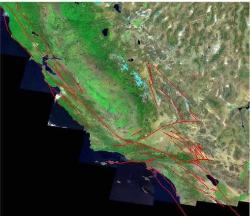
Virtual California includes the major strike-slip faults in California and is illustrated in Fig. 1. In this version of the model, Virtual California is composed of 650 fault

seg-10

ments, each of which has a width of 10 km and a depth of 15 km. A much more detailed treatment and explanation of the dynamics and equations solved numerically for Vir-tual California simulations can be found in (Rundle et al., 2004, 2005, and references therein).

An example of results from Virtual California is shown in Figs. 2a, b in which we

15

show two large earthquakes, one reminiscent of the San Francisco earthquake of 1906 (Fig. 2a) on the northern San Andreas fault, and one similar to the Fort Tejon earth-quake of 1857 on the southern San Andreas fault near the Big Bend between Fort Tejon and Wrightwood (Fig. 2b). In both Figs. 2a, b, red vertical bars represent “right lateral slip” (opposite side of the fault moves to the right) and blue vertical bars represent “left

20

lateral slip”.

It can be seen in Fig. 2a that the earthquake on the Northern San Andreas fault, where most of the slip occurs, also involves triggered slip on the Hayward, Rogers Creek and Maacama faults (these are the faults to the east of – “behind” – the main trace of the San Andreas fault). The dark bar on the San Andreas fault represents the

25

epicentral segment, the segment that was the first to slip in the event. The maximum amplitude of slip, as shown in the figure, is 9.3 m.

Figure 2b shows a large event in southern California similar in extent and magnitude to the 1857 Fort Tejon earthquake. It can be seen that while most of the slip occurs

HESSD

Full Screen / Esc

Printer-friendly Version Interactive Discussion on the main trace of the San Andreas fault, where the maximum amplitude of slip is

12.6 m, other triggered slip occurs on the Big Pine fault, the Garlock fault, the San Gabriel fault, and faults in the Mojave desert and Owens Valley to the east. In fact, it is extremely interesting that all of this activity began with initial slip on a small fault in the Mojave desert, as shown by the location of the dark epicentral vertical slip bar.

5

5 Patterns in Virtual California

We used 10 000 years of simulation data from Virtual California to compute the N=650 spatial patterns of activity for the simulation. These patterns reveal which are the most dominant and important modes of correlated activity, and which are less important. The eigenvectors (spectrum) indicate the fraction of the eigenvectors that are present, on

10

average, in the activity during the simulation. More specifically, p_n=λ2_n, is the fraction of eigenvector q_n(x) of the orthonormal N×N matrix Q of Eq. (7) is present, on average,

in the activity. Note that N P n₌₁

p_n=1. Using a frequency interpretation for probability, we can say that on average, over the 10 000 years of simulation data, the probability of finding eigenvector q_n(x) in the data is on average p_n.

15

In Figs. 3a, b, c, d we show the first four orthonormal correlation eigenvectors q_n(x),

again for the same 10 000 years of simulation data. In these figures, the red and blue bars correspond to locations where the value of q_n(x) is significantly different from 0.

The heights of the red and blue bars represent the values of q_n(x), and can take on

values between −1. and+1. Red bars represent positive values of q_n(x) between 10−3

20

and 1, and blue bars represent negative values of q_n(x) between −1 and −10−3. Green dashed lines are locations where |q_n(x) | has a value less than 10−3, which is roughly the amplitude of the numerical error. The physical meaning of the red and blue colors for a particular eigenvector q_n(x), which represents a particular fundamental pattern of

activity is:

HESSD

Full Screen / Esc

Printer-friendly Version Interactive Discussion

EGU

– Red sites tend to be active when other red sites are active, so that activity at red

sites is positively correlated with activity at other red sites;

– Blue sites tend to be active when other blue sites are active, so that activity at

blue sites is positively correlated with activity at other blue sites;

– Red sites tend to be inactive when the blue sites are active and vice-versa, so

5

that activity at red sites is negatively correlated with activity at other blue sites. Figure 3a is an eigenvector that represents the most important pattern of activity in the 10 000 years of simulation data. This pattern of activity comprises p₁=3.5%, on average, of the activity over 10 000 years of simulations. It bears a strong resemblance to Fig. 2b, the 1857-type event. From Fig. 3a, it can be seen that this pattern is

as-10

sociated with correlated activity on the San Andreas, the Garlock and Big Pine, the Northern Mojave, the Owens Valley and Death Valley faults. If one were to expand the pattern of slip in Fig. 2b as a sum of the eigenvectors q_n(x), the expansion coefficient

q₁(x) would represent the most important term.

Figure 3b shows the second-most important eigenvector q₂(x). Here we

primar-15

ily see strongly correlated activity on the northern San Andreas, the Hayward-Rogers Creek-Maacama, the Calaveras and Bartlett Springs fault systems. This pattern of activity is seen in 3.1% of the activity over the 10 000 years of simulations. This eigen-vector also resembles the event shown in Fig. 2a, the 1906-type event.

It is interesting that these first two patterns of activity are effectively decoupled

be-20

tween northern and southern California. The physical explanation for the decoupling is probably related to the existence of the creeping zone of the central San Andreas fault. This zone is the ∼100 km long part of the San Andreas fault just to the north of the large slipped region in Fig. 2b. Earthquakes do not occur in the creeping zone, rather a steady aseismic slip is observed at a rate corresponding to the long-term rate of plate

25

motion across the fault, 35 mm/yr (Table 1). The creeping zone appears to act as a kind of “shock absorber” for the largest events, effectively eliminating the correlation of these events in the north and south.

HESSD

Full Screen / Esc

Printer-friendly Version Interactive Discussion Eigenvectors 3 and 4 are shown in Figs. 3c and d. Figure 3c shows a pattern,

representing 2.4% of the activity, characterized by correlated slip on the southernmost part of the faults of the San Andreas system, together with slip activity on the eastern Garlock fault. Figure 3d is an interesting pattern, in which a kind of higher “pattern harmonic” of the activity on the faults of the northern San Andreas fault. Comparing

5

Figs. 3b and d, eigenvector 4 (1.8% of the activity) shows an anticorrelation between activity on the extreme northern end of the San Andreas system with the faults near the San Francisco Bay region (refer to Fig. 1 for locations relative to San Francisco). Eigenvector 4 also shows the beginnings of correlations between activity in northern California with activity south of the creeping zone, on the eastern Garlock fault in the

10

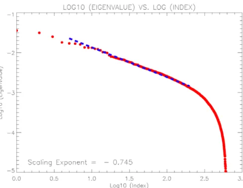
Mojave desert. Evidently the decoupling effect of activity in the north and south by the creeping zone of the San Andreas decreases as the higher pattern harmonics appear. Figure 4 shows the eigenvalue spectrum p_n. Here we plot Log₁₀ p_n as a function of Log₁₀n. We observe that there is a region of scaling or power-law behavior at values of n in the interval between n∼10 and n∼200:

15

Log₁₀p_n∝ −.75Log₁₀n(10 ≤ n ≤ 200) (8)

To understand this, we suppose that we can define a “characteristic wavelength” λ_n for each pattern according to the approximate ansatz:

λ_n∼ 2πL

n (9)

where L represents the linear size (length) of the largest events in the simulations.

20

Then the scaling region shown in Fig. 4 must be an expression of the hierarchical nature of the spatial scale of the patterns generated by the fault system dynamics:

p_n∼ λα_n ∼ n−α (10)

The reason for the particular value of the scaling exponent α=0.745±0.004≈0.75 is not at present known, but its value, which is nearly equal to the ratio of integers3_/3,

25

HESSD

Full Screen / Esc

Printer-friendly Version Interactive Discussion

EGU (Rundle, 1989; Rundle and Klein, 1993; Tiampo et al., 2002a). In mean field dynamics,

it is frequently the case that the scaling exponents are ratios of integers (see Klein et al., 2000).

We note that similar types of overall behavior for patterns has been observed in seismicity data (Tiampo et al., 2002b).

5

6 Conclusions

Forecasting in systems such as ENSO and earthquakes depends on the interpretation of observable space-time patterns, since the true stress-strain rate and stress-strain dynamics cannot be observed. It is likely that similar methods can be used for both systems, based upon the identification of patterns as eigenvectors of a dynamical

cor-10

relation operator. We note that these are linear descriptions of fundamentally nonlinear dynamical systems. However, there are important examples of of probability distribu-tions for nonlinear systems that are known to obey linear Fokker-Planck equadistribu-tions (Haken, 1983). Moreover, Klein et al. (2006)4 show that the evolution of patterns in driven threshold systems can be characterized by correlation functions that have the

15

properties discussed above.

We may speculate that hierarchical patterns that are observed in other nonlinear earth systems may be described in by similar methods. For example, it is known that in hydrology, river networks are observed to display scaling patterns that arise from purely local dynamics. These local dynamics include hill slope and topography, surface

20

winds and erosion, and rainfall. Yet these local effects are often the product of long range interactions, i.e., correlation of hill slope and topography, and rainfall patterns over long distances (Turcotte, 1997). Moreover, the tree-like nature of river networks leads also to the conjecture that pattern hierarchies may have a mean field character, inasmuch as tree-like networks are often found to be mean field constructs, such as

25

the Bethe lattice in percolation theory (Stauffer and Aharony, 1994). Understanding how these hierarchies of pattern scales develop and evolve doubtless holds the key to

HESSD

Full Screen / Esc

Printer-friendly Version Interactive Discussion forecasting the future dynamical states of these systems.

Acknowledgements. This work has been supported by grant DE-FG02-04ER15568 from the

U.S. Department of Energy, Office of Basic Energy Sciences to the University of California, Davis (J. B. Rundle, P. B. Rundle, G. Yakovlev); by grant DE-FG02-95ER14498 from the U.S. Department of Energy, Office of Basic Energy Sciences to the Boston University (W. Klein); 5

grant ATM 0327558 from the National Science Foundation (D. L. Turcotte, R. Shcherbakov); and by grants from the Computational Technologies Program of NASA’s Earth-Sun System Tech-nology Office to the Jet Propulsion Laboratory, the University of California, Davis (J. B. Rundle, P. B. Rundle, A. Donnellan).

References

10

Bowman, D. D., Ouillon, G., Sammis, C. G., Sornette, A., and Sornette, D.: An observational test of the critical earthquake concept, J. Geophys. Res., 103, 24 359–24 372, 1998.

Broomhead, D. S. and King, G. P.: Extracting qualitative dynamics from experimental data, Physica D, 20, 217–236, 1986.

Bufe, C. G. and Varnes, D. J.: Predictive modeling of the seismic cycle of the greater San 15

Francisco Bay region, J. Geophys. Res., 98, 9871–9883, 1993.

Crouch, S. L. and Starfield, A. M.: Boundary Element Methods in Solid Mechanics: with Ap-plications in Rock Mechanics and Geological Engineering, George Allen & Unwin, London, 1983.

Farrell, B.: Optimal excitation of neutral Rossby waves, J. Atmos. Sci., 45, 163–172, 1988. 20

Frankel, A. F.: Mapping seismic hazard in the Central and Eastern United States, Seismol. Res. Lett., 66, 8–21, 1995.

Garcia, A. and Penland, C.: Fluctuating hydrodynamics and principal oscillation pattern analy-sis, J. Stat. Phys., 64, 1121–1132, 1991.

Goes, S. D. B. and Ward, S. N.: Synthetic seismicity for the San Andreas Fault, Ann. Geofisica, 25

37, 1495–1513, 1994.

Haken, H.: Synergetics: An Introduction, Springer-Verlag, Berlin, 1983.

Holliday, J. R., Chen, C. C., Tiampo, K. F., Rundle, J. B., Turcotte, D. L., and Donnellan, A.: A RELM earthquake forecast based on pattern informatics, Seism. Res. Lett., in press, 2006.

HESSD

Full Screen / Esc

Printer-friendly Version Interactive Discussion

EGU

Holmes, P., Lumley, J. L., and Berkooz, G.: Turbulence, Coherent Structures, Dynamical Sys-tems and Symmetry, Cambridge University Press, Cambridge, UK, 1996.

Jordan, T. F.: Linear Operators for Quantum Mechanics, John Wiley, New York, 1969.

Kagan, Y. Y. and Jackson, D. D.: Probabilistic forecasting of earthquakes, Geophys. J. Int., 143, 438–453, 2000.

5

Karner, S. L. and Marone, C.: Effects of loading rate and normal stress on stress drop and stick-slip recurrence interval, in: GeoComplexity and the Physics of Earthquakes, edited by: Rundle, J. B., Turcotte, D. L., and Klein, W., Geophysical Monograph, 120, pp. 187–198, American Geophysical Union, Washington, D.C., 2000.

Keilis-Borok, V.: The lithosphere of the earth as a nonlinear system with implications for earth-10

quake prediction, Rev. Geophys., 28, 19–34, 1990.

Kerr, R. A. and Bagla, P.: A seismic murmur of what’s ahead for India, Science, 310, 208, 2005.

Keilis-Borok, V., Shebalin, P., Gabrielov, A., and Turcotte, D.: Reverse tracing of short-term earthquake precursors, Phys. Earth Planet. Int., 145, 75–85, 2004.

15

Klein, W., Anghel, M., Ferguson, C. D., Rundle, J. B., and Martins, J. S. S.: Statistical analysis of a model for earthquake faults with long-range stress transfer, in: GeoComplexity and the Physics of Earthquakes, edited by: Rundle, J. B., Turcotte, D. L., and Klein, W., Geophysical Monograph, 120, pp. 187–198, American Geophysical Union, Washington, D.C., 2000. Kossobokov, V. G., Keilis-Borok, V. I., Turcotte, D. L., and Malamud, B. D.: Implications of a 20

statistical physics approach for earthquake hazard assessment and forecasting, Pure Appl. Geophys., 157, 2323–2349, 2000.

Lay, T., Kanamori, H., Ammon, C. J., Nettles, M., Ward, S. N., Aster, R. C., Beck, S. L., Bilek, S. L., Brudzinski, M. R., Butler, R., DeShon, H. R., Ekstrom, G., Satake, K., and Sipkin, S.: The great Sumatra-Andaman earthquake of 26 December, 2004, Science, 308, 1127–1133, 25

2005.

Penland, C. and Sardeshmukh, P.: The optimal growth of tropical sea surface temperature anomalies, J. Climate, 8, 1999–2024, 1995.

Penland, C. and Magorian, T.: Prediction of Nino 3 sea surface termperatures using linear inverse modeling, J. Climate, 6, 1067–1075, 1993.

30

Penland, C. and Matrosova, L.: Studies of El Nino and interdecadal variability in tropical sea surface temperatures using a non-normal filter, J. Climate, in press, 2006.

HESSD

Full Screen / Esc

Printer-friendly Version Interactive Discussion

by: Mobley, C. D., Develop. Atmos. Sci., 17, Elsevier, Amsterdam, 1988.

Rundle, J. B.: A physical model for earthquakes, 2, Application to southern California, J. Geo-phys. Res., 93, 6255–6274, 1988.

Rundle, J. B.: A physical model for earthquakes: 3. Thermodynamical approach and its relation to nonclassical theories of nucleation, J. Geophys. Res., 94, 2839–2855, 1989.

5

Rundle, J. B. and Klein, W.: Scaling and critical phenomena in a class of slider block cellular automaton models for earthquakes, J. Stat. Phys., 72, 405–412, 1993.

Rundle, J. B., Rundle, P. B., Donnellan, A., and Fox, G.: Gutenberg-Richter statistics in topo-logically realistic system-level earthquake stress-evolution simulations, Earth Planets Space, 56, 761–771, 2004.

10

Rundle, J. B., Tiampo, K. F., Klein, W., and Martins, J. S. S.: Self-organization in leaky threshold systems: The influence of near-mean field dynamics and its implications for earthquakes, neurobiology, and forecasting, Proc. Nat. Acad. Sci., USA, 99, 2514–2521., Suppl. 1, 2002a. Rundle, J. B., Rundle, P. B., Klein, W., Martins, J. S. S., Tiampo, K. F., Donnellan, A., and

Kellogg, L. H.: Pure Appl. Geophys., 159, 2357–2381, 2002b. 15

Rundle, J. B., Rundle, P. B., Donnellan, A., and Fox, G.: Gutenberg-Richter statistics in topo-logically realistic system-level earthquake stress-evolution simulations, Earth Planets Space, 56, 761–771, 2004.

Rundle, J. B., Rundle, P. B., Donnellan, A., Turcotte, D., Shcherbakov, R., Li, P., Malamud, B. D., Grant, L. B., Fox, G. C., McLeod, D., Yakovlev, G., Parker, J., Klein, W., and Tiampo, K. F.: 20

A simulation-based approach to forecasting the next great San Francisco earthquake, Proc. Nat. Acad. Sci., 102, 15 363–15 367, 2005.

Rundle, J. B., Rundle, P. B., Donnellan, A., Li, P., Klein, W., Morein, G., Turcotte, D. L., and Grant, L.: Stress Transfer in Earthquakes and Forecasting: Inferences from Numerical Sim-ulations, Tectonophysics, 413, 109–125, doi:10.1016/j.tecto.2005.10031, 2006.

25

Rundle, P. B., Rundle, J. B., Tiampo, K. F., Martins, J. S. S., McGinnis, S., and Klein, W.: Nonlinear network dynamics on earthquake fault systems, Phys. Rev. Lett., 8714, Art. No. 148501, 2001.

Stauffer, D. and Aharony, A.: Introduction to Percolation Theory, Taylor and Francis, Bristol, PA, 1994.

30

Sykes, L. R. and Jaume, S. C.: Seismic activity on neighboring faults as a long-term precursor to large earthquakes in the San Francisco Bay area, Nature, 348, 595–599, 1990.

HESSD

Full Screen / Esc

Printer-friendly Version Interactive Discussion

EGU

systems and phase dynamics: An application to earthquake fault systems, Europhys. Lett., 60, 481–487, 2002a.

Tiampo, K. F., Rundle, J. B., Gross, S. J., McGinnis, S., and Klein, W.: Eigenpatterns in south-ern California seismicity, J. Geophys. Res., 107, B12, 2354, doi:10.1029/2001JB000562, 2002b.

5

Tiampo, K. F., Rundle, J. B., Klein, W., Martins, J. S. S., and Ferguson, C. D.: Ergodic dynamics in a natural threshold system, Phys. Rev. Lett., 91, 238 501(1–4), 2003.

Travis, J.: Scientists’ fears come true as hurricane floods New Orleans, Science, 309, 1656– 1659, 2005.

Tullis, T. E.: Rock friction and its implications for earthquake prediction examined via models of 10

Parkfield earthquakes, Proc. Nat. Acad. Sci. USA, 93, 3803–3810, 1996.

Turcotte, D. L.: Fractals and Chaos in Geology and Geophysics, 2nd Edition, Cambridge Uni-versity Press, Cambridge, UK, 1997.

Vautard, R. and Ghil, M.: Singular spectrum analysis in nonlinear dyanmics, with applications to paleoclimate time series, Physica D, 35, 395–424, 1989.

15

Ward, S. N.: An application of synthetic seismicity in earthquake statistics: the Middle America Trench, J. Geophys. Res., 97, 6675–6682, 1992.

Ward, S. N.: A synthetic seismicity model for southern California: Cycles, probabilities, hazards, J. Geophys. Res., 101, 22 393–22 418, 1996.

Ward, S. N.: San Francisco Bay Area earthquake simulations: A step toward a standard physi-20

cal earthquake model, Bull. Seis. Soc. Am., 90, 370–386, 2000.

Ward, S. N. and Goes, S. D. B.: How regularly do earthquakes recur – A synthetic seismicity model for the San Andreas fault, Geophys. Res. Lett., 20, 2131–2134, 1993.

HESSD

Full Screen / Esc

Printer-friendly Version Interactive Discussion

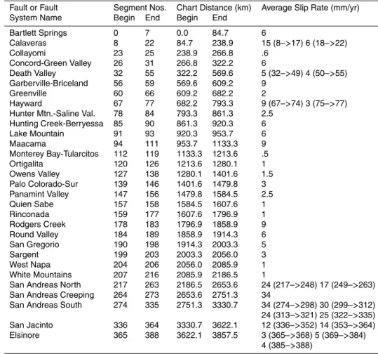
Table 1. Segments and geologic rates of offset for the modified version of VC 2001 used in

Figs. 1–4.

Fault or Fault Segment Nos. Chart Distance (km) Average Slip Rate (mm/yr) System Name Begin End Begin End

Bartlett Springs 0 7 0.0 84.7 6 Calaveras 8 22 84.7 238.9 15 (8–>17) 6 (18–>22) Collayomi 23 25 238.9 266.8 .6 Concord-Green Valley 26 31 266.8 322.2 6 Death Valley 32 55 322.2 569.6 5 (32–>49) 4 (50–>55) Garberville-Briceland 56 59 569.6 609.2 9 Greenville 60 66 609.2 682.2 2 Hayward 67 77 682.2 793.3 9 (67–>74) 3 (75–>77) Hunter Mtn.-Saline Val. 78 84 793.3 861.3 2.5

Hunting Creek-Berryessa 85 90 861.3 920.3 6 Lake Mountain 91 93 920.3 953.7 6 Maacama 94 111 953.7 1133.3 9 Monterey Bay-Tularcitos 112 119 1133.3 1213.6 .5 Ortigalita 120 126 1213.6 1280.1 1 Owens Valley 127 138 1280.1 1401.6 1.5 Palo Colorado-Sur 139 146 1401.6 1479.8 3 Panamint Valley 147 156 1479.8 1584.5 2.5 Quien Sabe 157 158 1584.5 1607.6 1 Rinconada 159 177 1607.6 1796.9 1 Rodgers Creek 178 183 1796.9 1858.9 9 Round Valley 184 189 1858.9 1914.3 6 San Gregorio 190 198 1914.3 2003.3 5 Sargent 199 203 2003.3 2056.0 3 West Napa 204 206 2056.0 2085.9 1 White Mountains 207 216 2085.9 2186.5 1

San Andreas North 217 263 2186.5 2653.6 24 (217–>248) 17 (249–>263) San Andreas Creeping 264 273 2653.6 2751.3 34

San Andreas South 274 335 2751.3 3330.7 34 (274–>298) 30 (299–>312) 24 (313–>321) 25 (322–>335) San Jacinto 336 364 3330.7 3622.1 12 (336–>352) 14 (353–>364) Elsinore 365 388 3622.1 3857.5 3 (365–>368) 5 (369–>384)

HESSD

Full Screen / Esc

Printer-friendly Version Interactive Discussion

EGU

Table 2. Continued.

Fault or Fault Segment Nos. Chart Distance (km) Average Slip Rate (mm/yr) System Name Begin End Begin End

Imperial Valley 389 406 3857.5 4020.0 30 Laguna Salada 407 416 4020.0 4118.5 4

Garlock 417 440 4118.5 4353.0–5 (417–>426)–7 (427–>440) Palos Verdes 441 447 4353.0 4428.6 3

Santa Cruz Island 448 452 4428.6 4481.9 −3 Brawley 453 457 4481.9 4533.8 25 Santa Monica 458 468 4533.8 4653.3 −3 Cleghorn 469 470 4653.3 4676.4 −3 Tunnel Ridge 471 472 4676.4 4695.6 −1.3 Helendale 473 481 4695.6 4781.7 .8 Lenwood-Lockhart 482 499 4781.7 4955.2 .8 Pipes Canyon 500 501 4955.2 4970.8 .7 Gravel Hills-Harper 502 509 4970.8 5051.2 .9 Blackwater 510 516 5051.2 5113.0 2 Camp Rock-Emerson 517 527 5113.0 5227.2 1 (517–>524) .6 (525–>527) Homestead Valley 528 530 5227.2 5254.4 .6 Johnson Valley 531 536 5254.4 5320.4 .6 Calico-Hidalgo 537 549 5320.4 5455.5 1 (537) 1.7 (538) 2.6 (539–>545) .6 (546–>549) Pisgah-Bullion 550 562 5455.5 5571.2 1 Mesquite Lake 563 564 5571.2 5592.2 1 Pinto Mountain 565 573 5592.2 5676.0 −1 Morongo Valley 574 574 5676.0 5690.6 −.5 Burnt Mountain 575 576 5690.6 5707.6.6 Eureka Peak 577 578 5707.6 5725.8 .6 Hollywood-Raymond 579 582 5725.8 5763.7 −1 (579–>580) −.5 (581–>582) Inglewood-Rose Cyn 583 604 5763.7 5979.2 1 (583->590) 1.5 (591->604) Coronado Bank 605 623 5979.2 6179.5 3 San Gabriel 624 637 6179.5 6310.8 3 (624–>628) 2 (630–>633) 1 (634–>637) Big Pine 638 644 6310.8 6379.5 −4 White Wolf 645 649 6379.5 6427.6 −5

HESSD

Full Screen / Esc

Printer-friendly Version Interactive Discussion

EGU

28

Figures

Fig. 1. Fault segments making up Virtual California. The model has 650 strike-slip fault

seg-ments, each approximately 10 km in length along strike and 15 km in depth.

HESSD

Full Screen / Esc

Printer-friendly Version Interactive Discussion

EGU

29

Fig. 2. Illustration of simulated earthquakes on the San Andreas fault. Two large earthquakes

are shown. Panel(a) is an event that is reminiscent of the San Francisco earthquake of 1906

on the northern San Andreas fault. Panel (b) is an event that is similar to the Fort Tejon

earthquake of 1857 on the southern San Andreas fault near the Big Bend between Fort Tejon and Wrightwood.

HESSD

Full Screen / Esc

Printer-friendly Version Interactive Discussion EGU 30 30 31 31

Fig. 3. This figure shows the first (and most important) four correlation eigenvectors for 10 000

years of simulation data. The color-coding of the vertical bars is that: 1) Red sites tend to be active when other red sites are active, so that activity at red sites is positively correlated with activity at other red sites; 2) Blue sites tend to be active when other blue sites are active, so that activity at blue sites is positively correlated with activity at other blue sites; 3) Red sites tend to be inactive when the blue sites are active and vice-versa, so that activity at red sites is negatively correlated with activity at other blue sites.

HESSD

Full Screen / Esc

Printer-friendly Version Interactive Discussion

EGU

32

Fig. 4. Plot of the eigenvalue spectrum pnon a log-log plot. Log10pnis plotted as a function of

Log₁₀n, where n is the index number of the eigenvector (n=1 has the largest value of pn, and

the rest are ordered by descending values of pn).