HAL Id: hal-00302932
https://hal.archives-ouvertes.fr/hal-00302932
Submitted on 23 Nov 2007
HAL is a multi-disciplinary open access
archive for the deposit and dissemination of
sci-entific research documents, whether they are
pub-lished or not. The documents may come from
teaching and research institutions in France or
abroad, or from public or private research centers.
L’archive ouverte pluridisciplinaire HAL, est
destinée au dépôt et à la diffusion de documents
scientifiques de niveau recherche, publiés ou non,
émanant des établissements d’enseignement et de
recherche français ou étrangers, des laboratoires
publics ou privés.
A simple conceptual model of abrupt glacial climate
events
H. Braun, A. Ganopolski, M. Christl, D. R. Chialvo
To cite this version:
H. Braun, A. Ganopolski, M. Christl, D. R. Chialvo. A simple conceptual model of abrupt glacial
climate events. Nonlinear Processes in Geophysics, European Geosciences Union (EGU), 2007, 14 (6),
pp.709-721. �hal-00302932�
www.nonlin-processes-geophys.net/14/709/2007/ © Author(s) 2007. This work is licensed
under a Creative Commons License.
Nonlinear Processes
in Geophysics
A simple conceptual model of abrupt glacial climate events
H. Braun1, A. Ganopolski2, M. Christl3, and D. R. Chialvo4
1Heidelberg Academy of Sciences and Humanities, c/o Institute of Environmental Physics, University of Heidelberg,
Im Neuenheimer Feld 229, 69120 Heidelberg, Germany
2Potsdam Institute for Climate Impact Research, P.O. Box 601203, 14412 Potsdam, Germany
3PSI/ETH Laboratory for Ion Beam Physics, c/o Institute of Particle Physics, ETH Zurich, 8093 Zurich, Switzerland 4Department of Physiology, Feinberg Medical School, Northwestern Univ., 303 East Chicago Ave. Chicago, IL 60611, USA
Received: 11 May 2007 – Revised: 4 October 2007 – Accepted: 5 November 2007 – Published: 23 November 2007
Abstract. Here we use a very simple conceptual model in an
attempt to reduce essential parts of the complex nonlinearity of abrupt glacial climate changes (the so-called Dansgaard-Oeschger events) to a few simple principles, namely (i) the existence of two different climate states, (ii) a threshold pro-cess and (iii) an overshooting in the stability of the system at the start and the end of the events, which is followed by a millennial-scale relaxation. By comparison with a so-called Earth system model of intermediate complexity (CLIMBER-2), in which the events represent oscillations between two climate states corresponding to two fundamentally different modes of deep-water formation in the North Atlantic, we demonstrate that the conceptual model captures fundamen-tal aspects of the nonlinearity of the events in that model. We use the conceptual model in order to reproduce and re-analyse nonlinear resonance mechanisms that were already suggested in order to explain the characteristic time scale of Dansgaard-Oeschger events. In doing so we identify a new form of stochastic resonance (i.e. an overshooting stochastic
resonance) and provide the first explicitly reported
manifes-tation of ghost resonance in a geosystem, i.e. of a mecha-nism which could be relevant for other systems with thresh-olds and with multiple states of operation. Our work enables us to explicitly simulate realistic probability measures of Dansgaard-Oeschger events (e.g. waiting time distributions, which are a prerequisite for statistical analyses on the regu-larity of the events by means of Monte-Carlo simulations). We thus think that our study is an important advance in or-der to develop more adequate methods to test the statistical significance and the origin of the proposed glacial 1470-year climate cycle.
Correspondence to: H. Braun
1 Introduction
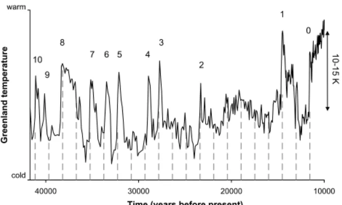
Time series of North Atlantic atmospheric/sea surface tem-peratures during the last ice age reveal the existence of re-peated large-scale warming events, the so-called Dansgaard-Oeschger (DO) events (Dansgaard et al., 1982; Grootes et al., 1993). In climate records from the North Atlantic region the events have a characteristic saw-tooth shape (Fig. 1): They typically start with a warming by up to 10–15 K (Severing-haus and Brook, 1999; Leuenberger et al., 1999) over only a few years/decades. Temperatures remain high for cen-turies/millennia until they drop back to pre-events values over a century or so. A prominent feature of DO events is their millennial time scale: During Marine Isotope Stages (MIS) 2 and 3, successive events in the GISP2 ice core were reported to be often spaced by about 1470 years or multiples thereof (Alley et al., 2001a; Schulz, 2002; Rahmstorf, 2003), compare Fig. 1. A leading spectral peak corresponding to the 1470-year period was found (Grootes and Stuiver, 1997; Yiou et al., 1997), and this spectral component was reported to be significant at least over a certain time interval (Schulz, 2002). We note, however, that the statistical significance of this pattern is still under debate (Ditlevsen et al., 2007), in particular because of the lack of adequate nonlinear analysis methods.
It was proposed that DO events represent rapid transi-tions between two fundamentally different modes of the ther-mohaline ocean circulation (THC) (Oeschger et al., 1984; Broecker et al., 1985), most likely corresponding to differ-ent modes of deep-water formation (Alley and Clark, 1999; Ganopolski and Rahmstorf, 2001). The origin of these transi-tions is also under debate: In principle they could have been caused by factors from outside of the Earth system (Keel-ing and Whorf, 2000; Rial, 2004; Clemens, 2005; Braun et al., 2005), but they could also represent internal oscilla-tions of the climate system (Broecker et al., 1990; Sakai and Peltier, 1997; van Kreveld et al., 2000). Several nonlinear
10000 20000
30000 40000
Time (years before present)
G re e n la n d te m p e ra tu re 0 1 2 3 4 5 6 7 8 9 10 warm cold 1 0 -1 5 K
Fig. 1. DO events as seen in the GISP2 ice-core from Greenland
(Grootes et al., 1993; Grootes and Stuiver, 1997). The figure shows Greenland temperature changes over the interval between 10000 and about 40000 years before present. DO events (0–10) manifest themselves as saw-tooth shaped warm intervals. Dashed lines are spaced by 1470 years.
resonance mechanisms have been suggested in order to ex-plain the characteristic timing of DO events, including co-herence resonance (Ganopolski and Rahmstorf, 2002; Tim-mermann et al., 2003; Ditlevsen et al., 2005) and stochastic resonance (Alley et al., 2001a,b; Ganopolski and Rahmstorf, 2002; Rahmstorf and Alley, 2002).
2 Spectrum of models
DO events have already been simulated by a variety of mod-els, ranging from simple conceptual ones to Earth system models of intermediate complexity (EMICs). Conceptual models are most suitable to perform large numbers of long-term investigations because they require very little compu-tational cost. However, they are often based on ad-hoc as-sumptions and only consider processes in a highly simplified way. In addition to that, the number of adjustable parame-ters is typically large compared to the degrees of freedom in those models. This implies that seemingly good results can often be obtained merely by excessive tuning. Nevertheless, conceptual models can provide important help for the inter-pretation of complex climatic processes.
The gap between conceptual models and the most com-prehensive general circulation models (GCMs), which are not yet applicable for millennial-scale simulations because of their large computational cost, is bridged by EMICs (Claussen et al., 2002). EMICs include most of the pro-cesses described in comprehensive models (in a more re-duced form), and interactions between different components of the Earth system (atmosphere, hydrosphere, cryosphere, biosphere, etc.) are simulated. The number of degrees of freedom typically exceeds the number of adjustable
param-eters by orders of magnitude. Since many EMICs are fast enough for studies on the multi-millennial time scale, they are the most adequate tools for the simulation of DO events.
3 The conceptual model
The simple conceptual model which we use here is an ex-tended version of the model described by Braun et al. (2005) (in the Supplementary Material of that publication). Here we use the model to demonstrate and analyse two appar-ently counterintuitive resonance phenomena (stochastic
res-onance and ghost resres-onance) that can exist in a large class of
highly nonlinear systems. Due to the complexity of many of those systems it is often impossible to precisely identify the reasons for the occurrence of these resonance phenomena. Our conceptual model, in contrast, has a very clear forcing-response relation as well as a very low computational cost and thus provides a powerful tool to explore these phenom-ena and to test their robustness. Furthermore, we describe and discuss the applicability of the model for improved statis-tical analyses (i.e. Monte-Carlo simulations) on the regular-ity of DO events. In the following the key assumptions of the conceptual model are first discussed. In the Supplementary Material we then compare the model performance under a number of systematic forcing scenarios with the performance of a more comprehensive model (the EMIC CLIMBER-2), compare Supplementary Information File and Supplemen-tary Figs. 1–6 (http://www.nonlin-processes-geophys.net/14/ 709/2007/npg-14-709-2007-supplement.pdf). In the frame-work of the conceptual model we finally demonstrate and interpret two hypotheses that were previously suggested in order to explain the recurrence time of DO events, and we discuss how these hypotheses could be tested.
3.1 Model description
Our conceptual model is based on three key assumptions: 1. DO events represent repeated transitions between two
different climate states, corresponding to warm and cold conditions in the North Atlantic region.
2. These transitions are rapid compared to the character-istic life-time of the two climate states (i.e. in first or-der approximation they occur instantaneously) and take place each time a certain threshold is crossed.
3. With every transition between the two states the thresh-old overshoots and afterwards approaches equilibrium following a millennial-scale relaxation process. This implies that the conditions for a switch between both states ameliorate with increasing duration of the cold and warm intervals.
Our three assumptions are supported by paleoclimatic ev-idence and/or by simulations with a climate model:
1. Since long, DO events have been regarded as repeated oscillations between two different climate states (Dans-gaard et al., 1982). It has been suggested that these states are linked with different modes of operation of the THC (Oeschger et al., 1984; Broecker et al., 1985). This seminal interpretation has since then influenced numerous studies and is now generally accepted (Rahm-storf, 2002). Indirect data indicate that the glacial THC indeed switched between different modes of operation (Sarnthein et al., 1994; Alley and Clark, 1999) which, according to their occurrence during cold and warm in-tervals in the North Atlantic, were labelled stadial and interstadial modes. A third mode named Heinrich mode (because of its presence during the so-called Heinrich events) is not relevant here.
2. High-resolution paleoclimatic data show that transitions from cold conditions in the North Atlantic region to warm ones often happened very quickly, i.e. on the decadal-scale or even faster (Taylor et al., 1997; Sev-eringhaus and Brook, 1999). The opposite transitions were slower, i.e. on the century-scale (Schulz, 2002), but nevertheless still faster that the characteristic life-time of the cold and warm intervals (which is on the cen-tennial to multi-millennial time scale, compare Fig. 1). The abruptness of the shifts from cold conditions to warm ones has commonly been interpreted as evidence for the existence of a critical threshold in the climate system that needs to be crossed in order to trigger a shift between stadial and interstadial conditions (Alley et al., 2003). Such a threshold could be provided by the THC (more precisely, by the process of deep-water formation): When warm and salty surface water from lower latitudes cools on its way to the North Atlantic, its density increases. If the density increase is large enough (i.e. if the surface gets denser than the deeper ocean water), surface water starts to sink. Otherwise, surface water can freeze instead of sinking. The onset of deep-water formation can thus hinder sea-ice forma-tion and facilitate sea-ice melting (due to the vertical heat transfer between the surface and the deeper ocean). A switch between two fundamentally different modes of deep-water formation can thus dramatically change sea ice cover and can cause large-scale climate shifts. Such nonlinear, threshold-like transitions between different modes of deep-water formation are at present consid-ered as the most likely explanation for DO events (Alley et al., 1999; Ganopolski and Rahmstorf, 2001).
3. The time-evolution of Greenland temperature during the warm phase of DO events has a characteristic saw-tooth shape (Fig. 1). Highest temperatures typically occur during the first decades of the events. These temper-ature maxima are followed by a gradual cooling trend over centuries/millennia, before the system returns to
cold conditions at the end of the events. This asym-metry supports the idea that the system overshoots in some way during the abrupt warming at the beginning of the events and that the subsequent cooling trend repre-sents a millennial-scale relaxation towards a new equi-librium (Schulz et al., 2002; Centurelli et al., 2006). We note that the time-evolution of Greenland temperature provides no clear evidence for an overshooting during the opposite transitions (i.e. from the warm state back to the cold one). This, however, is not necessarily in contradiction to our assumption: This lack of an over-shooting in the temperature fields does not necessarily mean that the ocean-atmosphere system did not over-shoot, since Greenland temperature evolution in the sta-dial state might have been dominated by factors other than the THC (respectively its stability), e.g. by Green-land ice accumulation, which would mask the signature of the THC in the ice core data.
We will show later (in Sect. 3.3.) that the assumption of an overshooting in the stability of the system is in fact strengthened by the analysis of model results obtained with the coupled model CLIMBER-2. In that model the overshooting results from the dynamics of the tran-sitions between the two climate states: In the stadial state deep convection occurs south of the Greenland-Scotland ridge (i.e. at about 50◦N). In the interstadial state, however, deep convection takes place north of the ridge (i.e. at about 65◦N). The onset of deep convection north of the Greenland-Scotland ridge, which releases accumulated energy to the atmosphere (i.e. heat that is stored mainly in the deep ocean), in first place starts DO events in the model. This heat release leads to a reduction of sea ice, which in turn further enhances sea surface densities between 50◦N and 65◦N (e.g. by in-creased local evaporation and reduced sea ice transport into that area). As a result deep convection also starts between 50◦N and 65◦N, and much more heat can be released to the atmosphere. Without a further response of the THC the system would return quickly (within years or decades, i.e. with the convective time scale) to its original state. In CLIMBER-2, however, the changes in deep convection trigger a northward extension and also an intensification of the ocean circulation (i.e. an overshooting of the Atlantic meridional overturning cir-culation; compare Ganopolski and Rahmstorf (2001)), which maintains the interstadial climate state since it is accompanied by an increase in the salinity and heat flux to the new deep convection area (at about 65◦N). In response to the overshooting of the overturning cir-culation, the system relaxes slowly (within about 1000 years, i.e. with the advective time scale) towards the sta-dial state. We note that the advective time scale corre-sponds to the millennial relaxation time in our concep-tual model. The model CLIMBER-2 also supports the
-1 0 1 F o rc in g f T h re s h o ld T A0 B0 B1 A1 -1 0 1 2 0 900 Time Mo d e l s ta te s S ta te v a ri a b le S t'' t'
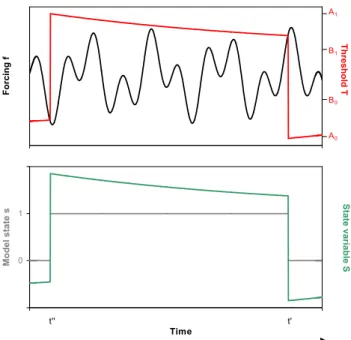
Fig. 2. Dynamics of our conceptual model. Shown is the time
evo-lution of the model, in response to a forcing that is large enough to trigger switches between both model states. Top: Forcing f (black) and threshold function T (red). Bottom: Model state s (grey; s=0 corresponds to the cold state, s=1 to the warm one) and state
vari-able S (green). At time t′′ the forcing falls below the threshold
function and a shift from the cold state into the warm one is trig-gered. With this transition, the threshold function switches to a non-equilibrium value (representing an overshooting of the system) and afterwards approaches equilibrium following a millennial-scale
relaxation. At time t′the forcing exceeds the threshold function,
and a transition from the warm state back into the cold one is trig-gered. With this transition, the threshold function switches to an-other non-equilibrium value and approaches equilibrium following another millennial-scale relaxation, until the forcing again falls be-low the threshold function and the next switch into the warm state is triggered. Note that the state variable S is chosen to be identical to the threshold function T . For convenience, discontinuities in T and
S are eliminated by linear interpolation. T , S and f are normalised
in the figure.
validity of our overshooting assumption during the op-posite transition (from the warm state back to the cold one), as we will show in Sect. 3.3. We would like to stress that our interpretation of the processes during DO events is, of course, not necessarily true since we can only speculate that the underlying mechanism of the events is correctly captured by CLIMBER-2.
3.2 Model formulation
We implement the above assumptions in the following way (compare Fig. 2): First we define a discrete index s(t) that indicates the state of the system at time t (in years). Since we postulate the existence of two states, s can only take two
values (s=1: warm state, s=0: cold state). We further define a threshold function T (t ) that describes the stability of the system at time t (i.e. the stability of the current model state). Second we define rules for the time evolution of the thresh-old function T . When the system shifts its state, we assume a discontinuity in the threshold function: With the switch from the warm state to the cold one (at time t′in Fig. 2) T takes the value A0. Likewise, with the switch from the cold state
into the warm one (at time t′′in Fig. 2) T takes the value A1.
As long as the system does not change its state the evolution of T is assumed to be given by a relaxation process:
dT
dt = −
(T − Bs)
τs
(1) (s labels the current model state, τs denotes the relaxation
time in that state, Bs is a state-dependent constant that
la-bels the equilibrium value of T in each model state). These assumptions result in the following expression for the thresh-old function T :
T (t ) = (As−Bs) · exp(−
t − δs
τs
) + Bs. (2)
Note that in the above expression the index s again denotes the current state of the model (i.e. s=0 stands for the cold state and s=1 for the warm one), δ0labels the time of the last
switch from the warm state into the cold one, and δ1indicates
the time of the last switch from the cold state into the warm one.
Third we assume that transitions from one state to the other are triggered each time a given forcing function f (t ) crosses the threshold function T . More precisely, we assume that when the system is in the cold state (s[t′′]=0) and the forcing
is smaller than the threshold value (f [t′′+1]<T [t′′+1]) the
system switches into the warm state (s[t′′+1]=1). This shift marks the start of a DO event. Likewise, when the system is in the warm state (s[t′]=1) and the forcing is larger than the threshold value (f [t′+1]>T [t′+1]) the system switches into the cold state (s[t′+1]=0). That shift represents the termina-tion of a DO event. If none of these conditermina-tions is fulfilled, the system remains in its present state (i.e. s[t+1]=s[t ]).
To simplify the comparison of the model output with pale-oclimatic records we further define a state variable S, which represents anomalies in Greenland temperature during DO events. For simplicity we assume that the state variable is equal to the threshold function: S(t )=T (t ) (i.e. we as-sume that Greenland temperature evolution during DO events is closely related to the current state of the THC, respec-tively to its stability). We stress that this assumption is of course highly simplified, because Greenland temperature is certainly not only influenced by the THC but also by other processes such as changes in ice accumulation during DO oscillations. However, this assumption is not crucial for the dynamics of our model, since the timing of the switches be-tween both model states is solely determined by the relation between the forcing function f and the threshold function T .
This means that even if we included a more realistic relation between T and S, the timing of the simulated climate shifts would be unchanged and the model dynamics would thus es-sentially be invariant.
Note that δ0 and δ1are not adjustable; they rather
repre-sent internal time markers. Thus, six adjustable parameters exist in our model as described here, namely A0, A1, B0, B1,
τ0and τ1. Our choice for these parameters is shown in
Ta-ble 1. With these parameter values the system is bistaTa-ble (i.e. no transition is ever triggered in the absence of any forcing, since B0≤0 and B1≥0) and almost symmetric. That means
that the average duration of the simulated warm and cold intervals is almost equal. When compared with Greenland paleotemperature records this situation most likely corre-sponds to the time interval between about 27 000 and 45 000 years before present, during which the duration of the cold and warm intervals in DO oscillations was also comparable (Fig. 1). The model can, however, also represent an unsta-ble (for B0>0 and B1<0) or a mono-stable system, in which
the stable state is either the warm one (for B0>0 and B1≥0)
or the cold one (for B0≤0 and B1<0); when compared to
the ice core data this situation is closer to the time inter-val between 15 000 and 27 000 years before present, since during that time the system was preferably in its cold state and the forcing apparently crossed the threshold only infre-quently and during short periods of time.
3.3 Comparison with a coupled climate model
In order to test our conceptual model we compare its per-formance under a number of systematic forcing scenarios with the performance of the far more comprehensive model CLIMBER-2 (a short description of that model is given in the Appendix; a detailed description exists in the publication of Petoukhov et al. (2000)).
Analogous to Braun et al. (2005), we investigate the re-sponse of both models to a forcing that consists of two century-scale sinusoidal cycles. In the conceptual model, the forcing is implemented as the forcing function f. In the EMIC, the forcing is added to the surface freshwater flux in the latitudinal belt 50–70◦N, following Ganopolski and Rahmstorf (2001) and Braun et al. (2005). This anomaly changes the vertical density gradient in the ocean and can thus trigger DO events. Switches from the cold state into the warm one are excited by sufficiently large (order of magni-tude: a few centimetre per year in the surface freshwater flux into the relevant area of the North Atlantic) negative fresh-water anomalies (i.e. by positive surface density anomalies that are strong enough to trigger buoyancy [deep] convec-tion), and the opposite switches are triggered by sufficiently large positive freshwater anomalies (i.e. by negative surface density anomalies that are strong enough to stop buoyancy [deep] convection). This justifies our choice for the logical relations that govern the dynamics of the transitions in the conceptual model (i.e. f (t )<T (t ) as the condition for the
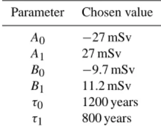
Table 1. Parameters of the conceptual model. All parameters have
the same values as in the publication of Braun et al. (2005). A0,
A1, B0and B1are given in freshwater units (i.e. in mSv =
milli-Sverdrup; 1 mSv=103m3/s), since the conceptual model was
orig-inally designed to mimic the response of the THC to an anomaly in the surface freshwater flux.
Parameter Chosen value
A0 −27 mSv A1 27 mSv B0 −9.7 mSv B1 11.2 mSv τ0 1200 years τ1 800 years
switch from the cold state to the warm one, f (t )>T (t ) for the opposite switch).
A detailed comparison between both model out-puts is presented in the Supplementary Material (http://www.nonlin-processes-geophys.net/14/709/2007/ npg-14-709-2007-supplement.pdf). We here only sum-marise the main results: We find a general agreement between both models, which is robust when the forcing parameters are varied over some range (Supplementary Figs. 1–6 – http://www.nonlin-processes-geophys.net/14/ 709/2007/npg-14-709-2007-supplement.pdf). The con-ceptual model reproduces the existence of three different regimes (cold, warm, oscillatory) in the output of the EMIC and also their approximate position in the forcing parameter-space. By construction only the nonlinear component in the response of the EMIC to the forcing is reproduced by the conceptual model (this component represents the saw-tooth shape of DO events). A second, more linear component is not included in the conceptual model (this component represents small-amplitude temperature anomalies which are superimposed on the saw-tooth shaped events in the EMIC). In particular, the conceptual model very well repro-duces the timing of the onset of DO events in the EMIC. The fact that our conceptual model, despite its simplicity, agrees in so many aspects with the much more detailed model CLIMBER-2 suggests that it indeed captures the key features in the dynamics of DO events in that model.
We would like to stress that the output of the EMIC indeed supports our assumption of an overshooting in the stability of the system during the transitions between both climate states: When driven by a periodic forcing (with a period of 1470 years), the EMIC can show pe-riodic oscillations during which it remains in either of its states for more than one forcing period (i.e. for con-siderably more than 1470 years, compare Supplementary Fig. 4a – http://www.nonlin-processes-geophys.net/14/709/ 2007/npg-14-709-2007-supplement.pdf). This implies that (at least in the EMIC) the conditions for a return to the
(a) 0 2940 5880 8820 Time (years) F o rc in g f Sta te v a ri a b le S - A1 - B1 - B0 - A0 0 0,1 0,2 0,3 0,4 0,5 0,6 0,7 0 5 10 15 20 Noise level σ (mSv) Relative frequency 0.1 0.2 0.3 0.4 0.5 0.6 (b)
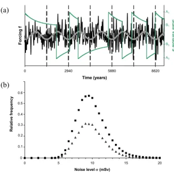
Fig. 3. Stochastic resonance. The input consists of: 1. a sub-threshold sinusoidal signal with a period of 1470 years and an
am-plitude of 4.5 mSv (about 40 percent of the threshold value B1
above which DO events occur in the model), 2. a random Gaussian-distributed signal with white noise power signature (standard devi-ation σ =8 mSv) and a cutoff frequency of 1/(50 years). The cutoff is used since no damping exists in the model and it thus shows an unrealistically large sensitivity to high-frequency (i.e. decadal-scale or faster) forcing. (a) Total input (black), periodic input compo-nent (grey), model output (green). Dashed lines are spaced by 1470 years. (b) Relative frequency to obtain a spacing of 1470 years
±10% (triangles) respectively ±20% (squares) between successive
events, as a function of the noise level σ .
opposite state indeed ameliorate with increased duration of the cold or warm intervals. If the thresholds in the model were constant (or gradually increasing with increasing dura-tion of the simulated cold/warm intervals), in contrast, the duration of the cold and warm intervals during the simu-lated oscillation could never be longer than 1470 years: If a periodic forcing does not cross a constant (or gradually in-creasing) threshold within its first period, it never crosses the threshold, due to the periodicity of the forcing.
4 Nonlinear resonance mechanisms in the model
Strongly nonlinear systems can show complex and appar-ently counterintuitive resonance phenomena that cannot oc-cur in simple linear systems. In this section we use our con-ceptual model to demonstrate and to discuss two of these phenomena, i.e. stochastic resonance (SR) and ghost reso-nance (GR). Since the explanation of the 1470-year cycle (and in fact even its significance) is still an open question,
we further discuss how future tests could distinguish between the proposed mechanisms.
4.1 Stochastic resonance (SR)
In linear systems that are driven by a periodic input, the exis-tence of noise generally reduces the regularity of the output (e.g. the coherence between the input and the output). This is not necessarily the case in nonlinear systems: Excitable or bistable nonlinear systems with a threshold and with noise, which are driven by a sinusoidal sub-threshold input, can show maximum coherence between the input and the output for an intermediate noise level, for which the leading out-put frequency of the system is close to the inout-put frequency. This phenomenon is called stochastic resonance (SR) (Benzi et al., 1982; Gammaitoni et al., 1998). SR has been suggested to explain the characteristic timing of DO events (Alley et al., 2001a), i.e. the apparent tendency of the events to occur with a spacing of about 1470 years or integer multiples thereof. It has further been demonstrated that DO events in the model CLIMBER-2 can be subject to SR (Ganopolski and Rahm-storf, 2002).
Here we apply our conceptual model to reproduce these results and to reanalyse the underlying mechanism. We use an input that is composed of: (i) a sinusoidal signal with a period of 1470 years, (ii) additional white noise. Figures 3 and 4 show that for a suitable noise level the model can in-deed show DO events with a preferred spacing of about 1470 years or integer multiples thereof. The reason for this pattern in the output is easily understandable in the context of the model dynamics: DO events in the model are triggered by pronounced minima of the total input (total input = periodic signal plus noise). These minima generally cluster around the minima of the sinusoidal signal, and the start of the sim-ulated events thus has a tendency to coincide with minima of the sinusoidal signal (Fig. 3a). Some minima of the si-nusoidal signal, however, are not able to trigger an event, because the magnitude of the noise around these minima is too small so that the threshold function is not reached by the total input. Consequently, a cycle is sometimes missed, and the spacing of successive events can change from about 1470 years to multiples thereof.
Unlike the model CLIMBER-2 (which has a complex re-lationship between the input and the output and also a large computational cost) our conceptual model can be used for a detailed investigation of the SR, e.g. because the dynam-ics of the model is simple and precisely known and because probability measures (such as waiting time distributions) can be explicitly computed. In fact, the resonant pattern in the conceptual model (Fig. 3) is due to two time-scale matching conditions: The noise level is such that the average waiting time between successive noise-induced transitions is compa-rable to half of the period of the periodic forcing, and also comparable to the relaxation times τ0 and τ1of the
0 500 1000 1500 2000 N u m b e r o f e v e n ts (a) 0 1000 2000 3000 4000 5000 (b) 0 500 1000 1500 2000 0 1470 2940 4410 5880 7350 8820 Spacing ∆T (years) N u m b e r o f e v e n ts 0 1000 2000 3000 4000 5000 0 1470 2940 4410 5880 7350 8820 Spacing ∆T (years) (d)
(c)
Fig. 4. Distribution of the spacing 1T between successive events. The input in (a) and (b) consists of noise only, with a standard deviation
σ of 8 mSv (as in Fig. 3a). In (c) and (d), a sinusoidal input component (amplitude=4.5 mSv, period=1470 years; compare Fig. 3) is added
to the noise. In (a) and (c) the threshold function is constant in each state (20 mSv in the warm state and −20 mSv in the cold one), while the overshooting relaxation assumption is used in (b) and (d) (with threshold parameters as shown in Table 1). Thus, c corresponds to the “usual” SR while d shows our “overshooting” SR.
from the usual SR, in which thresholds (or potentials) are constant in time (apart from the influence of the periodic in-put). In the usual SR, only one time-scale matching condi-tion exists (Gammaitoni et al., 1998), namely the one that the average waiting time between successive noise-induced transitions (i.e. the inverse of the so-called Kramers rate) is comparable to half of the period of the periodic forcing.
In order to investigate the implications of the second con-dition we simulate histograms for four different scenarios in the conceptual model (Fig. 4): 1. noise-only input, con-stant threshold (Fig. 4a); 2. noise-only input, overshooting threshold (Fig. 4b); 3. noise plus periodic input, constant threshold (Fig. 4c); 4. noise plus periodic input, overshoot-ing threshold (Fig. 4d). We note that 3. corresponds to the usual SR, while 4. describes our overshooting stochastic
res-onance. As can be seen from the histograms, the existence
of the millennial-scale relaxation process leads to a synchro-nisation in the sense that the waiting times between succes-sive events are confined within a much smaller time interval (about 1000–4500 years with the overshooting, compared to about 0–10 000 years without overshooting).
This confinement is plausible since the transition proba-bility between both model states strongly depends on the magnitude of the threshold, which declines with increasing duration of the cold or warm intervals: When the standard deviation of the noise level is chosen such that the aver-age waiting time between successive noise-induced transi-tions is comparable to the relaxation times τ0 and τ1, as in
Fig. 4, the overshooting relaxation strongly reduces the tran-sition probability for waiting times much smaller than the relaxation time (since the corresponding values of the thresh-old function are large) and increases the transition probabil-ity for waiting times of the order of the relaxation time or larger (since the corresponding values of the threshold func-tion are considerably smaller). The probability to find an only century-scale spacing between successive events is thus small, because the corresponding transition probabilities are small. On the other hand, the probability to find a multi-millennial spacing is also small, because the states are al-ready depopulated before (i.e. the probability to obtain life-times considerably larger than the relaxation time is almost zero). This explains why the possible values for the spac-ing between successive DO events are restricted to a much smaller range than in the usual SR (i.e. in the case with con-stant thresholds).
This synchronisation effect is indeed not unique to the con-ceptual model: The output of the coupled model CLIMBER-2 shows a similar pattern (with possible waiting times be-tween successive DO events of e.g. about 1500–5000 years or about 1000–3000 years, depending on the noise level; com-pare Fig. 4a–d in the publication of Ganopolski and Rahm-storf (2002)). This similarity is of course not surprising, since the conceptual model is apparently able to mimic the events in the EMIC and since an overshooting in the stabil-ity of both states clearly also exists in CLIMBER-2 (com-pare Sect. 3.3). We note that in the GISP2 ice core data,
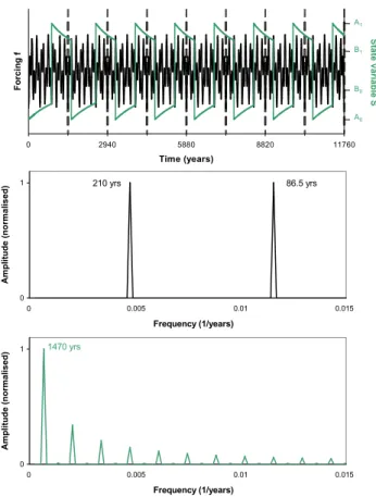
0 2940 5880 8820 11760 Time (years) F o rc in g f S ta te v a ri a b le S A1 B1 B0 A0 0 1 Frequency (1/years) A m p li tu d e (n o rm a li s e d ) 210 yrs 0.01 0.015 0 0.005 86.5 yrs 0 1 Frequency (1/years) A m p li tu d e (n o rm a li s e d ) 1470 yrs 0.01 0.015 0 0.005
Fig. 5. Ghost resonance. Top: Forcing (black) and model re-sponse (green). Middle: Amplitude spectrum of the forcing. Bot-tom: Amplitude spectrum of the model response. We use two sinusoidal forcing cycles, with frequencies of 7/(1470 years) and 17/(1470 years), respectively, and with equal amplitudes. These two cycles coincide every 1470 years and create peaks of particu-larly pronounced magnitude, spaced by exactly that period. Thus, despite the fact that there is no spectral power at the correspond-ing frequency (see middle panel), the forccorrespond-ing repeatedly crosses the threshold at those intervals. Consequently, the response of the con-ceptual model (i.e. the time evolution of the state variable S) shows strictly repetitive DO events with a period of 1470 years (as indi-cated by the dashed lines, which are spaced by 1470 years). Despite the lack of a 1470-year spectral component in the forcing, the output shows a very prominent peak at the corresponding frequency.
DO events in the time interval 27 000–45 000 years before present (which, as discussed in Sect. 3.2, is the best analogue to the “background climate state” in our conceptional model, since the duration of the cold and warm intervals in the data is comparable in that interval) have spacings of about 1000– 3000 years (compare Fig. 1) and were reported to cluster around values of either about 1470 years or about 2940 years (Schulz, 2002). Because the SR mechanism could explain such a pattern (compare Fig. 4d) it has originally been pro-posed. However, this mechanism requires a sinusoidal input with a period of about 1470 years, which has so far not been detected.
4.2 Ghost resonance (GR)
In linear systems which are driven by a periodic input, the frequencies of the output are always identical to the input frequencies. This is not necessarily the case in nonlinear sys-tems. For example, nonlinear excitable (or bistable) systems that are driven by an input with frequencies corresponding to harmonics of a fundamental frequency (which itself is not present in the input) can show a resonance at the fundamen-tal frequency, i.e. at a frequency with zero input power. This phenomenon, which was first described in order to explain the pitch of complex sounds (Chialvo et al., 2002; Chialvo, 2003) and later observed experimentally e.g. in laser systems (Buldu et al., 2003), is called ghost resonance (GR). GR and SR can indeed occur in the same class of systems, e.g. in bistable or excitable systems with thresholds. However, un-like SR, GR requires a periodic driver with more than one frequency. Although many geophysical systems might be subject to GR (since the relevant processes often have thresh-olds), the occurrence of this mechanism has so far not ex-pressly been demonstrated in geoscience.
Here we discuss a hypothesis that was recently proposed to explain the 1/(1470 years) leading frequency of DO events (Braun et al., 2005). The underlying mechanism of the hy-pothesis is in fact the first reported manifestation of GR in a geophysical model system. According to that hypothesis the 1/(1470 years) frequency of DO events could represent the nonlinear climate response to forcing cycles with frequen-cies close to harmonics of 1/(1470 years). Our conceptual model illustrates the plausibility of this mechanism: We use a bi-sinusoidal input with frequencies of 7/(1470 years) and 17/(1470 years), i.e. with frequencies corresponding to the 7th and the 17th harmonic of a 1/(1470 years) fundamental frequency, and with equal amplitudes. A spectral component corresponding to the fundamental frequency is not explicitly present in the input. Since the two sinusoidal cycles corre-spond to harmonics of the missing fundamental, the input signal repeats with a period of 1470 years. For an appro-priate range of input amplitudes, the output of the concep-tual models shows periodic DO events with a period of 1470 years (Fig. 5). Unlike the input, the model output exhibits a pronounced frequency of 1/(1470 years), corresponding to the leading frequency of DO events and to the fundamental frequency that is absent in the input. This apparent para-dox is explained by the fact that the two driving cycles enter in phase every 1470 years, thus creating pronounced peaks spaced by that period. Because the magnitude of these peaks results from constructive interference of the two driving cy-cles, it is indeed robust that a threshold process can be much more sensitive to these peaks than to the two original driving cycles (Chialvo, 2003).
The main strength of the GR mechanism is that – unlike the SR mechanism – it can relate the leading frequency of DO events to a main driver of natural (non-anthropogenic) climate variability, since proxies of solar activity suggest
the existence of solar cycles with periods close to 1470/7 (=210) years (De Vries or Suess cycle) and 1470/17 (≈86.5) years (Gleissberg cycle) (Stuiver and Braziunas, 1993; Wag-ner er al., 2001; Peristykh and Damon, 2003). So far, how-ever, no empirical evidence for this mechanism has been found (Muscheler and Beer, 2006), nor has it been shown yet that changes in solar activity over the solar cycles are sufficiently strong to actually trigger DO events.
In order to investigate the stability of this mechanism we further add a stochastic component (i.e. white noise) to the forcing. In this case the events are – of course – not strictly periodic anymore. Similar to the SR case, an optimal (i.e. intermediate) noise level exists for which the waiting time distribution of the simulated events exhibits a maximum at a value of 1470 years, corresponding to the period of the fundamental frequency of the two input cycles (Fig. 6). In contrast to the SR case, in which a fairly simple waiting time distribution with a few broad maxima of century scale width is obtained (compare Fig. 4d), we now find a much more complex pattern with a large number of very sharp lines of only decadal scale width. Since the waiting time distribu-tions of both mechanisms are considerably different, it could – at least in principle – be possible to distinguish between both mechanisms by analysing the distribution of the ob-served DO events. In practise, however, this approach is complicated by the fact that only about ten events appear to be sufficiently well dated for this kind of analysis, and even their spacing has an uncertainty of about 50 years (Ditlevsen et al., 2007), which is already of the same order as the width of the peaks in Fig. 6b. We note that the mechanism that is described in Fig. 6 is known as ghost stochastic resonance (GSR), and its occurrence and robustness has already been reported before in other systems with thresholds and multi-ple states of operation (Chialvo, 2003). At least in our sys-tem, however, this mechanism is even more complex than the other two types of resonance (SR, GR). It is beyond the scope of this paper to describe the GSR mechanism in more detail.
4.3 Testing the proposed mechanisms
The most direct way to test which of the proposed mech-anisms – if any – provides the correct explanation for the timing of DO events would be to reconstruct decadal-scale density anomalies in the North Atlantic in connection with the events. This is not possible since even the most highly resolved oceanic records do not allow to reconstruct the vari-ability of the glacial ocean on that time scale. Thus, only in-direct tests can be performed. The identification of the postu-lated 1/(1470 years) forcing frequency, which has so far not been detected, would certainly give further support for the SR mechanism. And in order to support the GR mechanism, it remains crucial to demonstrate that century-scale solar ir-radiance variations are indeed of sufficiently large amplitude to trigger repeated transitions (with a preferred time scale
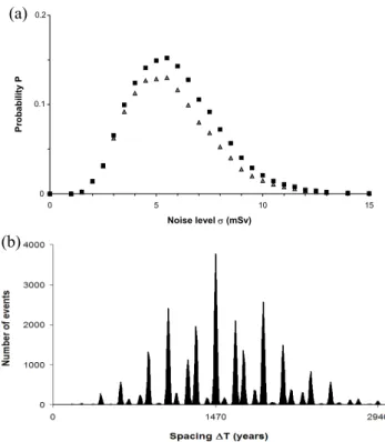
0 0,1 0,2 0 5 10 15 Noise level σ (mSv) Pr o b a b il it y P 0.1 0.2 (a) (b)
Fig. 6. Ghost stochastic resonance. The input consists of: 1. two
sinusoidal forcing cycles with frequencies of 7/(1470 years) and 17/(1470 years), respectively, and with an amplitude of 8 mSv, 2. a random Gaussian-distributed signal with white noise power sig-nature and a cutoff frequency of 1/(50 years), as in Fig. 3. In (a), the relative frequency to obtain a spacing of 1470 years ±1% (tri-angles) respectively ±2% (squares) between successive events is shown as a function of the noise level σ . (b) shows the distribution of the spacing 1T between successive events (standard deviation of the noise: 5.5 mSv).
of about 1470 years) between the two glacial climate states. This could be tested with climate models.
An elegant and simple test is to make use of the observa-tion that DO events in the Earth system model CLIMBER-2 represent the nonlinear response to the forcing, and that an additional (and much smaller) linear response is superim-posed on the events. In the absence of any threshold crossing (e.g. in the Holocene, during which DO events did not oc-cur) the response to the forcing, in contrast, does not show a strong nonlinear component. This suggests that Holocene climate archives from the North Atlantic region might be able to reveal what triggered glacial DO events. This approach has two major advantages: First, more reliable (e.g. better resolved and dated) records are available to solve this issue. Second, linear analysis methods can be used for that pur-pose, e.g. linear correlations. In the context of the GR mech-anism, for example, the existence of a pronounced correla-tion between Holocene climate indices from the North At-lantic and solar activity proxies (reconstructed e.g. from14C
variations in precisely dated tree rings) would be expected. Up to now at least one study exists that supports this pre-diction of a linear relationship between century-scale solar forcing and North Atlantic climate variability throughout the Holocene: Proxies of drift ice anomalies in the North At-lantic show a persistent correlation and a statistically signifi-cant coherency with “rapid (100- to 200-year), conspicuously large-amplitude variations” in solar activity proxies (Bond et al., 2001), in accordance with the proposed GR mecha-nism.
The most challenging test, however, is the direct analysis of the glacial climate records. We are convinced that one of the main difficulties in this approach is the high degree of nonlinearity of the events, which – according to our in-terpretation – has so far not been adequately addressed in many previous studies. For example, several attempts have already been made in order to investigate the 1470-year cy-cle by means of linear spectral analysis methods, and signif-icance levels have commonly been calculated by assuming a red noise background. To us this assumption seems to be oversimplified, since the system responds at a preferred time scale even when driven by white noise (compare Fig. 4b). We thus suspect that the significance levels obtained by this method are unrealistically high. We further think that the re-ported lack of a clear phase relation between solar activity proxies and DO events (Muscheler and Beer, 2006) cannot rule out the idea that solar forcing synchronised DO events, since in the case of an additional stochastic forcing compo-nent (i.e. in the GSR case) the events are triggered by the
combined effect of solar forcing and noise. Thus, the
ob-served lack could also imply that only some of the events were in first place triggered by the Sun, whereas others were caused mainly by random variability (e.g. by noise).
A new and promising approach, which is based on a Monte-Carlo method, has recently been proposed in order to test the significance of the glacial 1470-year climate cy-cle: Ditlevsen et al. (2007) define a certain measure in or-der to distinguish between different hypotheses for the tim-ing of DO events, and they explicitly calculate the value of this measure for the series of events observed in the ice core. They then compare the calculated value with the values ob-tained by several hypothetic processes, e.g. by a random pro-cess (for which assumptions concerning the probability dis-tribution of the recurrence times of the events have to be made). Significance levels are obtained from the (numeri-cally estimated) probability distributions of the measure as generated by the considered process. Although we do not share their conclusions (because we think that more adequate measures can be chosen, which give considerably different results) we think that this approach is elegant because signif-icance levels are not calculated based on linear theories. The method is thus also applicable to highly nonlinear time series. A major hurdle in this method is that for each considered pro-cess the probability distribution of the waiting times – which is unknown for almost all processes – somehow has to be
specified. For example, Ditlevsen et al. (2007) use a sim-ple mathematical (i.e. an exponential) distribution in order to mimic random DO events. In order to improve their novel approach, some method is thus needed to calculate waiting time distributions in response to any possible input. Com-prehensive models are not applicable, due to their large com-putational cost. Our conceptual model, in contrast, is well designed for that purpose because it is combines the ability to mimic the complex nonlinearity of DO events as described by an accepted Earth system model with the extremely low computational cost of a very simple (zeroth order) model. We thus think that our work is an important step in order to develop improved statistical analysis methods which are able to cope with the extreme nonlinearity of DO events.
5 Discussion and conclusions
We here discussed DO events in the framework of a very simple conceptual model that is based on three key as-sumptions, namely (i) the existence of two different cli-mate states, (ii) a threshold process and (iii) an overshoot-ing in the stability of the system at the start and the end of the events, which is followed by a millennial-scale re-laxation. These assumptions are in accordance with pale-oclimatic records and/or with simulations performed with CLIMBER-2, a more complex Earth system model. In a couple of systematic tests we showed (in the Supple-mentary Material – http://www.nonlin-processes-geophys. net/14/709/2007/npg-14-709-2007-supplement.pdf) that de-spite its simplicity, our model very well reproduces DO events as simulated with CLIMBER-2, whose dynamics is based on a (albeit reduced) description of the underlying hydro-/thermodynamic processes. The correspondence be-tween both models thus strengthens our interpretation that the conceptual model can successfully mimic key features of DO events, and that these can be regarded as a new type of non-equilibrium oscillation (i.e. as an overshooting
relax-ation oscillrelax-ation) between two states of a nonlinear system
with a threshold.
Although we discussed our model dynamics in the con-text of the (thermohaline) ocean circulation, our model does not explicitly assume that DO events are linked with changes in the ocean circulation: Threshold behaviour and multiple states exist in many compartments of the climate system (not only in the ocean, but e.g. also in the atmosphere and in the cryosphere). Our model thus cannot rule out a leading role of non-oceanic processes in DO oscillations. The millennial time scale of the events (which is represented in our model by the assumption of a millennial-scale relaxation), however, corresponds to the characteristic time scale of the thermoha-line circulation and thus points to a key role of the ocean in DO oscillations.
The main strength of our model is its simplicity: Due to the obvious relationship between forcing and response,
the model can demonstrate why even a simple bistable (or excitable) system with a threshold can respond in a com-plex way to a simple forcing, which consists of only one or two sinusoidal inputs and noise. We applied our model to discuss two highly nonlinear and apparently counterin-tuitive resonance mechanisms, namely stochastic resonance and ghost resonance. In doing so we reported a new form of stochastic resonance (i.e. an overshooting stochastic
res-onance), in which the overshooting of the system leads to a
further synchronisation effect compared to the usual stochas-tic resonance. Our study provides the first explicitly reported manifestation of ghost resonance in a geophysical (model) system. Since threshold behaviour and multiple equilibria are not unique to DO events but exist in many geophysical systems, we would indeed expect that ghost resonances could be inherent in many geosystems and not just in our model.
In addition to its applicability to demonstrate and inter-pret nonlinear resonance mechanisms, and to test their stabil-ity, we further illustrated the ability of our conceptual model to simulate probability measures (e.g. waiting time distri-butions, which are required in order to test the significance and the cause of the proposed glacial 1470-year climate cy-cle by means of Monte-Carlo simulations). Because it com-bines the ability to reproduce essential aspects of DO events with the extremely low computational cost of a conceptual model (which is up to 107times lower than in the Earth sys-tem model CLIMBER-2), we think that our model represents an important advance in order to develop adequate nonlinear methods for improved statistical analyses on DO events.
Appendix A
Description of CLIMBER-2
The Earth system model CLIMBER-2, which we used for our analysis, has dynamic components of the atmosphere, of the oceans (including sea ice) and the vegetation. Dynamic ice sheets were not included in our study. CLIMBER-2 is a global model with coarse resolution: For the atmosphere and the continents the spatial resolution is 10◦ in latitude, and 7 sectors are considered in longitude. The ocean is zonally averaged with a latitudinal resolution of 2.5◦ for the three large ocean basins. A detailed description of the model is given in the publication of Petoukhov et al. (2000).
DO events in the model represent abrupt switches between two different climate states (stadial [i.e. cold] and
intersta-dial [i.e. warm]), corresponding to two different modes of
the THC: In the interstadial mode, North Atlantic deep water (NADW) forms at about 65◦N and much of the North At-lantic is ice-free. In the stadial mode, NADW forms at about 50◦N and a considerably larger area of the North Atlantic is ice-covered. We note that for the climatic background con-ditions of the Last Glacial Maximum (LGM) only the stadial mode is stable in the model whereas the interstadial mode
is excitable but unstable (Ganopolski and Rahmstorf, 2001). Moreover, the stability of both modes depends on the actual climate state (e.g. on the configuration of the Laurentide ice sheet and on the freshwater input into the North Atlantic), and the stability properties of the system change when the background conditions are modified (more precisely, the sys-tem can be bistable or mono-stable).
Transitions between both modes can be triggered by anomalies in the density field of the North Atlantic, for ex-ample by variations in the surface freshwater flux (since the density of ocean water increases with increasing salinity). In our study we thus implement the forcing as a perturbation in the freshwater flux (in the latitudinal belt 50–70◦N): We start the model with the climatic background conditions of the Last Glacial Maximum (LGM). Following earlier sim-ulations (Braun et al., 2005) we then add a small constant offset of −17 mSv (1 mSv=103m3/s) to the freshwater flux.
For this climate state (which we label perturbed LGM) the THC is in fact bistable and DO events can be triggered more easily than for LGM conditions. This perturbed LGM state gives us the background conditions for the model simulations as presented in this paper.
Acknowledgements. The authors thank R. Calov, A. Mangini,
S. Rahmstorf, K. Roth and A. Witt for discussion, and P. Ditlevsen (in particular for observing the difference between the usual stochastic resonance and our overshooting stochastic resonance) and two anonymous reviewers for helpful comments. H. Braun was funded by Deutsche Forschungsgemeinschaft, DFG project number MA 821/33.
Edited by: H. A. Dijkstra
Reviewed by: P. Ditlevsen and two other anonymous referees
References
Alley, R. B. and Clark, P. U.: The deglaciation of the northern hemi-sphere: A global perspective, Ann. Rev. Earth Planet. Sci., 27, 149–182, 1999.
Alley, R. B., Clark, P. U., Keigwin, L. D., and Webb, R. S.: Mak-ing sense of millennial-scale climate change, in: Mechanisms of Global Climate Change at Millennial Time Scales, edited by: Clark, P. U., Webb, R. S., and Keigwin, L. D., AGU, Washington, DC, 385–394, 1999.
Alley, R. B., Anandakrishnan, S., and Jung, P.: Stochastic resonance in the North Atlantic, Paleoceanography, 16, 190–198, 2001a. Alley, R. B., Anandakrishnan, S., Jung, P., and Clough, A.:
Stochas-tic resonance in the North AtlanStochas-tic: Further insights, in: The Oceans and Rapid Climate Change: Past, Present and Future, edited by Seidov, D., Maslin, M., Haupt, B. J., AGU, Washing-ton, DC, 57–68, 2001b.
Alley, R. B., Marotzke, J., Nordhaus, W. D., Overpeck, J. T., Pe-teet, D. M., Pielke Jr., R. A., Pierrehumbert, R. T., Rhines, P. B., Stocker, T. F., Talley, L. D., and Wallace, J. M.: Abrupt Climate Change, Science, 299, 2005–2010, 2003.
Benzi, R., Parisi, G., Sutera, A., and Vulpiani, A.: Stochastic reso-nance in climatic change, Tellus, 34, 10–16, 1982.
Bond, G., Kromer, B., Beer, J., Muscheler, R., Evans, M. N., Show-ers, W., Hoffmann, S., Lotti-Bond, R., Hajdas, I., and Bonani, G.: Persistent Solar Influence on North Atlantic Climate During the Holocene, Science, 294, 2130–2136, 2001.
Braun, H., Christl, M., Rahmstorf, S., Ganopolski, A., Mangini, A., Kubatzki, C., Roth, K., and Kromer, B.: Possible solar origin of the 1,470-year glacial climate cycle demonstrated in a coupled model, Nature, 438, 208–211, 2005.
Broecker, W. S., Peteet, D. M., and Rind, D.: Does the ocean-atmosphere system have more than one stable mode of opera-tion?, Nature, 315, 21–26, 1985.
Broecker, W. S., Bond, G., Klas, M., Bonani, G., and Wolfli, W.: A salt oscillator in the glacial Atlantic? 1. The concept, Paleo-ceanography, 5, 469–477, 1990.
Buldu, J. M., Chialvo, D. R., Mirasso, C. R., Torrent, M. C., and Garcia-Ojalvo, J.: Ghost resonance in a semiconductor laser with optical feedback, Europhys. Lett., 64, 178–184, 2003.
Centurelli, R., Musacchioa, S., Pasmanterc, R. A., and Vulpiani, A.: Resemblances and differences in mechanisms of noise-induced resonance, Physica A, 360, 261–273, 2006.
Chialvo, D. R., Calvo, O., Gonzalez, D. L., Piro, O., and Savino, G. V.: Subharmonic stochastic synchronization and resonance in neuronal systems, Phys. Rev. E, 65, 050902, doi:10.1103/PhysRevE.65.050902, 2002.
Chialvo, D. R.: How we hear what is not there: A neuronal mech-anism for the missing fundamental illusion, Chaos, 13, 1226– 1230, 2003.
Claussen, M., Mysak, L. A., Weaver, A. J., Crucifix, M., Fichefet, T., Loutre, M.-F., Weber, S. L., Alcamo, J., Alexeev, V. A., Berger, A., Calov, R., Ganopolski, A., Goose, H., Lohmann, G., Lunkeit, F., Mokhov, I. I., Petoukhov, V., Stone, P., and Wang, Z.: Earth system models of intermediate complexity: closing the gap in the spectrum of climate system models, Clim. Dynam., 18, 579–586, 2002.
Clemens, S. C.: Millennial-band climate spectrum resolved and linked to centennial-scale solar cycles, Quat. Sci. Rev., 24, 521– 531, 2005.
Dansgaard, W., Clausen, H. B., Gundestrup, N., Hammer, C. U., Johnsen, S. F., Kristinsdottir, P. M., and Reeh, N.: A New Green-land Deep Ice Core, Science, 218, 1273–1277, 1982.
Ditlevsen, P. D., Kristensen, M. S., Andersen, K. K.: The recur-rence time of Dansgaard-Oeschger events and possible causes, J. Climate, 18, 2594–2603, 2005.
Ditlevsen, P. D., Andersen, K. K., Svensson, A.: The DO-climate events are probably noise induced: statistical investigation of the claimed 1470 years cycle, Clim. Past, 3, 129–134, 2007, http://www.clim-past.net/3/129/2007/.
Gammaitoni, L., H¨anggi, P., Jung, P., and Marchesoni, F.: Stochas-tic resonance, Rev. Mod. Phys., 70, 223–288, 1998.
Ganopolski, A. and Rahmstorf, S.: Simulation of rapid glacial cli-mate changes in a coupled clicli-mate model, Nature, 409, 153–158, 2001.
Ganopolski, A. and Rahmstorf, S.: Abrupt glacial climate changes due to stochastic resonance, Phys. Rev. Lett., 88, 038501, doi:10.1103/PhysRevLett.88.038501, 2002.
Grootes, P. M., Stuiver, M., White, J. W. C., Johnsen, S., and Jouzel, J.: Comparison of oxygen isotope records from the GISP2 and GRIP Greenland ice cores, Nature, 366, 552–554, 1993. Grootes, P. M. and Stuiver, M.: Oxygen 18/16 variability in
Green-land snow and ice with 103to 105-year time resolution, J.
Geo-phys. Res., 102, 26 455–26 470, 1997.
Keeling, C. D. and Whorf, T. P.: The 1,800-year oceanic tidal cycle: A possible cause of rapid climate change, Proc. Natl. Acad. Sci. USA, 97, 3814–3819, 2000.
Leuenberger, M., Schwander, J., and Johnsen, S.: 16◦C Rapid
Tem-perature Variations in Central Greenland 70,000 Years Ago, Sci-ence, 286, 934–937, 1999.
Muscheler, R. and Beer, J.: Solar forced
Dans-gaard/Oeschger events?. Geophys. Res. Lett., 33, L20706, doi:10.1029/2006GL026779, 2006.
Oeschger, H., Beer, J., Siegenthaler, U., Stauffer, B., Dansgaard, W., and Langway Jr., C. C.: Late glacial climate history from ice cores, in: Climate Processes and Climate Sensitivity, edited by: Hansen, J. E. and Takahashi, T., AGU, Washington, DC, 299– 306, 1984.
Peristykh, A. N. and Damon, P. E.: Persistence of the Gleiss-berg 88-yr solar cycle over the last 12,000 years: Evidence from cosmogenic isotopes, J. Geophys. Res., 108(A1), 1003, doi:10.1029/2002JA009390, 2003.
Petoukhov, V., Ganopolski, A., Brovkin, V., Claussen, M., Eliseev, A., Kubatzki, C., and Rahmstorf, S.: CLIMBER-2: A climate system model of intermediate complexity. Part I: Model descrip-tion and performance for present climate, Clim. Dynam., 16, 1– 17, 2000.
Rahmstorf, S.: Ocean circulation and climate during the past 120,000 years, Nature, 419, 207–214, 2002.
Rahmstorf, S.: Timing of abrupt climate change: a precise clock, Geophys. Res. Lett., 30, 1510–1514, 2003.
Rahmstorf, S. and Alley, R. B.: Stochastic resonance in glacial cli-mate, EOS, 83, 129–135, 2002.
Rial, J. A.: Abrupt Climate Change: Chaos and Order at Orbital and Millennial Scales, Global Planet. Change, 41, 95–109, 2004. Sakai, K. and Peltier, W. R.: Dansgaard-Oeschger oscillations in a
coupled atmosphere-ocean climate model, J. Climate, 10, 949– 970, 1997.
Sarnthein, M., Winn, K., Jung, S. J. A., Duplessy, J. C., Labeyrie, L., Erlenkeuser, H., and Ganssen, G.: Changes in East Atlantic Deepwater Circulation over the Last 30,000 Years: Eight Time Slice Reconstructions, Paleoceanography, 9, 209–267, 1994. Schulz, M.: On the 1470-year pacing of Dansgaard-Oeschger warm
events. Paleoceanography, 17, 1014–1022, 2002.
Schulz, M., Paul, A., and Timmermann, A., Relaxation oscilla-tors in concert: A framework for climate change at millennial timescales during the late Pleistocene, Geophys. Res. Lett., 29, 2193–2197, 2002.
Severinghaus, J. P. and Brook, E.: Abrupt Climate Change at the End of the Last Glacial Period Inferred from Trapped Air in Polar Ice, Science, 286, 930–934, 1999.
Stuiver, M. and Braziunas, T. F.: Sun, ocean, climate and atmo-spheric CO2: An evaluation of causal and spectral relationships, Holocene, 3, 289–305, 1993.
Taylor, K. C., Mayewski, P. A., Alley, R. B., Brook, E. J., Gow, A. J., Grootes, P. M., Meese, D. A., Saltzman, E. S., Sever-inghaus, J. P., Twickler, E. S., White, J. W. C., Whitlow, S., and Zielinski, G. A.: The Holocene-Younger Dryas Transition Recorded at Summit, Greenland, Science, 278, 825–827, 1997. Timmermann, A., Gildor, H., Schulz, M., and Tziperman, E.,
by Massive Meltwater Pulses, J. Climate, 16, 2569–2585, 2003. van Kreveld, S. A., Sarnthein, M., Erlenkeuser, H., Grootes, P.,
Jung, S., Nadeau, M. J., Pflaumann, U., and Voelker, A.: Po-tential links between surging ice sheets, circulation changes and the Dansgaard-Oeschger cycles in the Irminger Sea, 60–18 kyr, Paleoceanography, 15, 425–442, 2000.
Wagner, G., Beer, J., Masarik, J., Muscheler, R., Kubik, P. W., Mende, W., Laj, C., Raisbeck, G. M., and Yiou, F.: Presence of the solar de Vries cycle (≈205 years) during the last ice age, Geophys. Res. Lett., 28, 303–306, 2001.
Yiou, P., Fuhrer, K., Meeker, L. D., Jouzel, J., Johnsen, S., and Mayewski, P. A.: Paleoclimatic variability inferred from the spectral analysis of Greenland and Antarctic ice-core data, J. Geophys. Res., 102, 26 441–26 454, 1997.