HAL Id: hal-01983460
https://hal.archives-ouvertes.fr/hal-01983460
Submitted on 16 Jan 2019
HAL is a multi-disciplinary open access
archive for the deposit and dissemination of
sci-entific research documents, whether they are
pub-lished or not. The documents may come from
teaching and research institutions in France or
abroad, or from public or private research centers.
L’archive ouverte pluridisciplinaire HAL, est
destinée au dépôt et à la diffusion de documents
scientifiques de niveau recherche, publiés ou non,
émanant des établissements d’enseignement et de
recherche français ou étrangers, des laboratoires
publics ou privés.
Efficient Algorithms to Test Digital Convexity
Loïc Crombez, Guilherme da Fonseca, Yan Gerard
To cite this version:
Loïc Crombez, Guilherme da Fonseca, Yan Gerard. Efficient Algorithms to Test Digital Convexity.
21st IAPR International Conference on Discrete Geometry for Computer Imagery, DGCI 2019, Mar
2019, Paris, France. �hal-01983460�
Efficient Algorithms to Test Digital Convexity
Lo¨ıc Crombez
Universit´
e Clermont Auvergne and
LIMOS
Clermont-Ferrand, France
[email protected]
Guilherme D. da Fonseca
Universit´
e Clermont Auvergne and
LIMOS
Clermont-Ferrand, France
[email protected]
Yan G´
erard
Universit´
e Clermont Auvergne and
LIMOS
Clermont-Ferrand, France
[email protected]
Abstract
A set S ⊂ Zd is digital convex if conv(S) ∩ Zd = S, where conv(S) denotes the convex hull of S. In this paper, we consider the algorithmic problem of testing whether a given set S of n lattice points is digital convex. Although convex hull computation requires Ω(n log n) time even for dimension d = 2, we provide an algorithm for testing the digital convexity of S ⊂ Z2 in O(n + h log r) time, where h is the number of edges of the convex hull and r is the diameter of S. This main result is obtained by proving that if S is digital convex, then the well-known quickhull algorithm computes the convex hull of S in linear time. In fixed dimension d, we present the first polynomial algorithm to test digital convexity, as well as a simpler and more practical algorithm whose running time may not be polynomial in n for certain inputs.
1
Introduction
Digital geometry is the field of mathematics that studies the geometry of points with integer coor-dinates, also known as lattice points [1]. Convexity is a fundamental concept in digital geometry, as well as in continuous geometry [2]. From a historical perspective, the study of digital convexity dates back to the works of Minkowski [3] and it is the main subject of the mathematical field of geometry of numbers.
While convexity has a unique well stated definition in any linear space, different definitions have been investigated in Z2
and Z3 [4, 5, 6, 7, 8]. In two dimensions, we encounter at least five different
approaches, called respectively digital line, triangle, line [4], HV (for Horizontal and Vertical [9]), and Q (for Quadrant [10]) convexities. These definitions were created in order to guarantee that a digital convex set is connected (in terms of the induced grid subgraph), which simplifies several algorithmic problems.
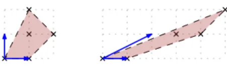
The original definition of digital convexity in the geometry of number does not guarantee connec-tivity of the grid subgraph, but provides several other important mathematical properties, such as being preserved under certain affine transformations (Fig. 1). The definition is the following. A set of lattice points S ⊂ Zd
is digital convex if conv(S) ∩ Zd= S, where conv(S) denotes the convex hull
of S.
Herein, we consider the fundamental problem of verifying whether a given set of lattice points is digital convex.
Problem TestConvexity(S)
Input: Set S ⊂ Zd of n lattice points given by their coordinates.
Output: Determine whether S is digital convex or not.
The input of TestConvexity(S) is an unstructured finite lattice set (without repeating elements). Related work considered more structured data in dimension 2, in which S is assumed to be connected.
Figure 1: Shearing a digital convex set. Example of a set whose connectivity is lost after a linear shear.
The contour of a connected set S of lattice points is the ordered list of the points of S having a grid neighbor outside S. When S is connected, it is possible to represent S by its contour, either directly as in [11] or encoded as binary word [12]. The algorithms presented in [11, 12] test digital convexity in linear time on the respective input representations.
Our work, however, does not make any assumption on S being connected, or any particular ordering of the input. In this setting, a naive approach to test the digital convexity is:
1. Compute the convex hull conv(S) of the n lattice points of S. 2. Compute the number n0 of lattice points inside the convex hull of S. 3. If n = n0, then S is convex. Otherwise, it is not.
Step 1 consists of computing the convex hull of n points. The field of computational geometry provides a plethora of algorithms to compute the convex hull of a finite set S ⊂ Rd of n points [13].
The fastest algorithms for dimensions 2 and 3 take O(n log n) time [14], which matches the lower bound in the algebraic decision tree model of computation [15]. In dimension d ≤ 3, if we also take into consideration the output size h, i.e. the number of vertices of the convex hull, the fastest algorithms take O(n log h) time [16, 17]. Some polytopes with n vertices (e.g., the cyclic polytope) have Θ(nb(d−1)/2c) facets. Therefore, any algorithm that outputs this facet description of the convex
hull requires Ω(nb(d−1)/2c) time. Optimal algorithms to compute the convex hull in dimension d ≥ 4
match this lower bound [18].
Step 2 consists of computing the number of lattice points inside a polytope (represented by its vertices), which is a well studied problem. In dimension 2, it can be solved using Pick’s formula [19]. The question has been widely investigated in the framework of the geometry of numbers, from Ehrhart theory [20] to Barvinok’s algorithm [21]. Currently best known algorithms have a complexity of O(nO(d)) for fixed dimension d [22]. As conclusion, the time complexity of this naive approach is at
least the one of the computation of the convex hull.
1.1
Results
In Section 2, we consider the 2-dimensional version of the problem and show that the convex hull of digital convex sets can be computed in linear time. Our main result is an algorithm for dimension d = 2 to solve TestConvexity(S) in O(n + h log r) time, where h is the number of edges of the convex hull and r is the diameter of S.
In Section 3, we consider the problem in fixed dimension d. We present the first polynomial-time algorithm to test digital convexity, as well as a simpler and more practical algorithm whose running time may not be polynomial in n for certain inputs.
2
Digital Convexity in 2 Dimensions
The purpose of this section is to provide an algorithm to test the convexity of a finite lattice S ⊂ Z2
in linear time in n. To this endeavour, we show that the convex hull of a digital convex set S can be computed in linear time. In fact, we show that this linear running time is achieved by the well-known quickhull algorithm [23].
Quickhull is one the many early algorithms to compute the convex hull in dimension 2. Its worst case time is O(n2), which makes it generally less attractive than the O(n log n) algorithm. However for
certain inputs and variations of the algorithm, the average time complexity is reduced to O(n log n) or O(n) [13, 24].
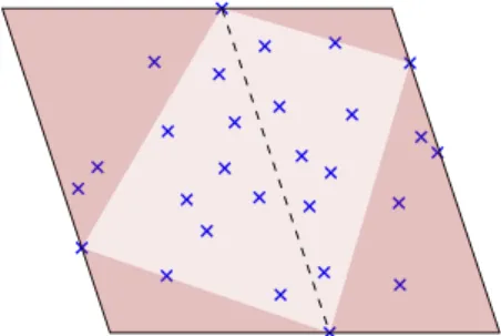
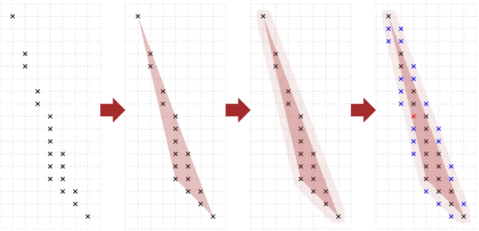
Figure 2: Quickhull initialization. Points inside the partial hull (light brown) are discarded. The remaining points are potentially part of the hull.
The quickhull algorithm starts by initializing a convex polygon in the following manner. First it computes the top-most and bottom-most points of the set. Then it computes the two extreme points in the normal direction of the line supported by the top-most and bottom-most points. Those four points describe a convex polygon that we call a partial hull, which is contained inside the convex hull of S. The points contained in the interior of the partial hull are discarded. Furthermore, horizontal lines and lines parallel to the top-most to bottom-most line passing through these points describe an outlying bounding box in which the convex hull lies (Fig. 2).
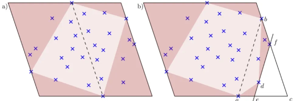
The algorithm adds vertices to the partial hull until it obtains the actual convex hull. This is done by inserting new vertices in the partial hull one by one. Given an edge of the partial hull, let v denote its outwards normal vector. The algorithm searches for the extreme point in direction v. If this point is already an edge point, then the edge is part of the convex hull. Otherwise, we insert the farthest point found between the two edge vertices, discarding the points that are inside the new partial hull. Throughout this paper, we call a step of the quickhull algorithm the computation of the farthest point of every edge for a given partial hull. When adding new vertices to the partial hull, the region inside the partial hull expands. Points inside that expansion are discarded by quickhull and herein we name this region discarded region. The points that still lie outside the partial hull are preserved, and we call the region within which points might still lies preserved region (Fig. 3).
We show that quickhull steps takes linear time and that at each step half of the remaining input points of the convex hull is discarded. Therefore, as in standard decimation algorithms, the total running time remains linear. In Section 2.2, we explain how to use this algorithm to test the digital convexity of any lattice set in linear time in n.
Theorem 1. If the input is a digital convex set of n points, then QuickHull has O(n) time and space complexities.
2.1
Proof of Theorem 1
We prove Theorem 1 with the help of the following lemma.
Lemma 2. The area of the discarded region is larger than the area of the preserved region.
Proof. Consider one step of the algorithm: Let ab be the edge associated to the step. When a was added to the hull, it was as the farthest point in a given direction. Hence, there is no point behind the line orthogonal to this direction going through a. (Fig. 3b). The same can be said for b. Let c be the intersection point of those two lines. Every point that lies within 4abc will be fed to the following steps. At this step, we are looking for the point that is the farthest from the supporting line of ab and outside the partial hull (let that point be d) (Fig. 4). Let e and f be the intersections between the line parallel to ab going through d, and respectively ac and bc. There are no points from S inside the triangle 4cef . Adding d to the partial hull creates two other edges to further be treated: one with ad as an edge that will be fed the points inside 4ade and one with bd as the edge that will be fed the points inside 4bdf . The triangle 4abd lies within the partial hull, therefore 4abd is the region in which points are discarded. (Fig. 4)
a c d b f e a) b)
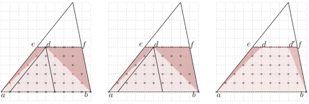
Figure 3: Quickhull regions. The preserved region (region in which we look for the next vertex to be added to the partial hull) is a triangle. This stays true when adding new vertices to the hull (as shown here in the bottom right corner). The partial hull (whose interior is shown in light brown) grows at each vertex insertions to the partial hull. The new region added to the partial hull is called discarded region. c f e d c1 c2 a e1 f2 b
Figure 4: Symmetrical regions.The next step of the algorithm will only be fed the points inside the dark brown regions (search regions). Each lattice points inside the light brown region (discarded region) is inside the partial hull and is therefore discarded. Each search region (in dark brown) has a symmetrical region (either through c1 or c2) that lies inside the discarded region. Furthermore, this
symmetrical transformation also preserve lattice points.
the discarded lattice points are those within 4abd. Let c1 be the middle of ad and c2 be the middle
of bd. As shown in Fig. 4, the symmetrical of 4ade and 4bdf through respectively c1 and c2
both lie inside 4abd and do not intersect each other. Hence 4abd is larger in terms of area than 4aed ∪ 4bdf .
Remark 1. Pick’s formula does not apply here since all vertices of the triangle (namely c in Fig. 4) are not necessarily lattice points.
Remark 2. As there is no direct relation between the area of a triangle and the number of lattice points inside it, this result is not sufficient to conclude that a constant proportion of points are discarded at each step.
Corollary 3. The reflection of lattice points inside 4aed and 4bdf across respectively c1 and c2 are
lattice points.
Proof. The points a, b, d are lattice points so c1 and c2 (middle of respectively ad and bd) have their
coordinates in multiple of half integers. Hence the reflection of a lattice point across c1 or c2 is a
lattice point. Therefore, every lattice point within 4aed has a lattice point reflection across c1within
a b d e f a b e d f a b e d d0f
Figure 5: Lonely points. The lattice points without discarded symmetrical counterparts are shown in red. On the left: if every points inside the triangle is preserved, and in the center: if the points on the edges of the partial hull are discarded. Finally on the right a visualization of what happens if we discard all the farthest points and update the partial hull accordingly.
Remark 3. This previous result would prove that half the points are discarded at each step if it were not for the lattice points on the diagonals ad and bd.
We will now show that quickhull discards at least half of the remaining points at each step, hence proving theorem 1
Proof. We established in Corollary 3 that lattice points inside the search regions (4aed and 4bf d) have symmetrical counterparts inside the discarded region (more precisely inside 4ae1d and 4bf2d)
(Fig. 4). By preserving each points inside 4aed and 4bf d at each step, we do not have a discarded symmetrical counterpart for the lattice points lying on ad and bd. But we do not need to preserve those points, since ad and bd are at this step edges of the partial hull. Removing lattice points from ad and bd implies that in the following step there will be no lattice points on ab, leaving lattice points on ef without a discarded symmetrical counterparts (Fig. 5).
Let actually discard every points on ef , since they all are equally farthest from ab in the outer direction, they all belong to the hull. Hence we can add the first and last lattice point on ef to the partial hull (Fig. 5). Note that this only takes linear time and does not change the time complexity of each individual step. Hence, at each step of quickhull, for every preserved points there is at least a discarded point. Consequently, the number of operations is proportional to n
∞ P i=0 (1 2) i = 2n and
quickhull takes linear time for digital convex sets.
2.2
Determining the digital convexity of a set
We showed in Theorem 1 that the quickhull algorithm computes the convex hull of digital convex sets in linear time thanks to the fact that at each step quickhull discards at least half of the remaining points. By running quickhull on any given set S, and stopping the computation if any step of the algorithm discards less than half of the remaining points, we ensure both that the running time is linear, and that if S is digital convex, quickhull finishes and we get the convex hull of S. If the computation finishes for S, we still need to test its digital convexity. To do so, we use the previously computed convex hull and compute |conv(S) ∩ Z2| using Pick’s formula [19]. The set S is digital convex if |conv(S) ∩ Z2| = |S|. Hence the resulting Algorithm 1.
Theorem 4. Algorithm 1 tests digital convexity of any 2 dimensional set S, and runs in O(n+h log r) time, where h is the number of edges of conv(S) and r is the diameter of S.
Proof. As Algorithm 1 runs quickhull, but stops as soon as less than half the remaining points have been removed, the running time of the quickhull part is bounded by the series n
∞ P i=0 (1 2) i = 2n, and
is hence linear. Thanks to Theorem 1 we know that the computation of quickhull will not stop for any digital convex sets. Computing |conv(S) ∩ Z2| using Pick’s formula requires the computation of
Algorithm 1 isDigitalConvex(S) Input: S a set of points
Output: true if S is digital convex, false if not.
1: while S is not empty do
2: Run one step of the quickhull algorithm on S
3: if quickhull discarded less than half the remaning points of S then
4: return false
5: Compute |conv(S) ∩ Z2| 6: if |conv(S) ∩ Z2| > |S| then 7: return false
8: return true
the area of conv(S) and of the number of lattice points lying on its boundary, which requires the computation of a greatest common divisor. Hence this takes O(h log r) time where h is the number of edge of conv(S) and r is the diameter of S. As S is digital convex if and only if |S| = |conv(S) ∩ Z2|,
Algorithm 1 effectively tests the digital convexity of a 2 dimensional set in O(n + h log r) time.
3
Test Digital Convexity in Dimension d
We provide two algorithms for verifying the digital convexity in any fixed dimension.
3.1
Naive algorithm
The naive algorithm mentioned in the Introduction is based on the following equivalence: the set S ⊂ Zd
is digital convex if and only if its cardinality is equal to the cardinality of conv(S) ∩ Zd. In
Step 1, we compute the convex hull of S (in O(n log n + nbd2c) time [18]). In Step 2, we need to count
the number of integer points inside conv(S). The classical algorithm to achieve this goal is known as Barvinok algorithm [21]. This approach determines only the number of missing points. If we want to enumerate the points, it is possible to do so through a formal computation of the generating functions used in Barvinok algorithm.
Theorem 5. The naive algorithm tests digital convexity in any fixed dimension d and runs in poly-nomial time.
Proof. Computing the convex hull of any set can be done in O(n log n + nbd2c) time [18]).
Count-ing lattice points inside a convex lattice polytope can be done in polynomial time [22]. A direct consequence of the digital convexity definition is that a set S ⊂ Zd is digital convex if and only if |S| = |conv(S) ∩ Zd|, hence the naive algorithm tests digital convexity in any fixed dimension d and
runs in polynomial time.
3.2
Alternative algorithm
This new algorithm computes all integer points in the convex hull of S with a more direct approach. Its principle is to enumerate the points x of a finite lattice set S0 ⊂ Zd
surrounding conv(S) ∩ Zd (conv(S) ∩ Zd ⊂ S0). In a first variant, we count the number of points of S0 belonging to conv(S).
At the end, the set S is convex if and only if |conv(S) ∩ Zd| is equal to the cardinality of S. In a second variant, for each point of S0, we test whether it belongs to S and in the negative case, we
test whether it belongs to the convex hull of S. If a point of S0\ S ∩ conv(S) is found, then S is not
convex.
We define the set S0 as the set of points x ∈ Zd such that the cube x + [−1 2,
1 2]
d has a nonempty
intersection with the convex hull of S, where + denotes the Minkowski sum. It can be easily proved that S0 is 2d-connected (the 2d neighbors of a lattice point x ∈ Zd are the 2d integer points at
Euclidean distance 1) and by construction, it contains S. The graph structure induced by the 2d-connectivity on S0 allows to visit all the points of S0 efficiently: for each point x ∈ S0, we consider
Figure 6: Practical algorithm. A lattice set S, its convex hull and its dilation by a centered cube of side 1. The intersection of conv(S) + [−12,12]d with the lattice is the set S0. It is 2d-connected and
contains the convex hull of S. The principle of the algorithm is either to count the points of S0 in conv(S) (variant 1) or to search for a point of S0\ S (blue points) in the convex hull of S (variant 2).
its 2d neighbors and test whether they belong to S0. If they do, we add them to the stack of the remaining points of S0. The goal is to test whether a point of S0\ S is in the convex hull of S.
Then the algorithm has two main routines:
• InConvexHullS tests whether a given point x ∈ Rd belongs to the convex hull of S. It is
equivalent with testing whether there exists a hyperplane separating x from the points of S. It can be done by linear programming with a worst-case time complexity of O(n) for fixed dimension d [13].
• InConvexHullS+[−1
2,12]dtests whether a given point x belongs to the convex hull of S +[− 1 2,
1 2]
d.
It follows the same principle as InConvexHullS with 2dn points. The time complexity remains
linear in fixed dimension. This routine is used to test whether an integer point belongs to S0. The algorithm is the following. First, we create a stack T of the points of S0 to visit and initialize it with the set S. For each point x in T , we remove it from the stack T and label it as already visited. Then, we consider its 2d neighbors x0. If x0belongs to S0and has not been visited previously, we add it in the stack T . We test whether x belongs to conv(S) and increment the cardinality of conv(S) ∩ Zd accordingly (variant 1) or test whether x is in S and conv(S) and return S not convex
if x ∈ conv(S) \ S (variant 2).
The running time is strongly dependent on the cardinality of S0. It is O(n|S0|). If the size of S0
is of the same magnitude as the initial set, the algorithm runs in O(n2) time. It is unfortunately not possible to bound |S0| as a function of n. The ratio |S|S|0| can go to infinity. It is easy to build such an example with a set S consisting of only two lattice points, for instance for any k ∈ Z the set S = {(0, 0); (1, 2k)} induces |S|S|0| ≥ k. A direction of improvement could be to consider a linear transformation of the lattice Zd in order to obtain a more compact lattice set and then a lower ratio
|S0|
|S|. LLL algorithm [25] could be useful to achieve this goal in future work.
As in the naive algorithm, a variant of this approach can be easily developed in order to enumerate the missing points.
4
Perspectives
In this paper, we presented an algorithm to test digital convexity in time linear in n for dimension d = 2. In higher dimensions, our running time depends on the complexity of general convex hull algorithms. The questions of whether digital convexity can be tested in linear time in 3 dimensions,
or faster than convex hull computation in arbitrary dimensions remain open. A tentative approach consists of changing the lattice base, in order to obtain certain connectivity properties.
We showed that the convex hull of a digital convex set in dimension 2 can be computed in linear time. Can the convex hull of digital convex sets be computed in linear time in dimension 3, or more generally, what is the complexity of convex hull computation of a digital convex set in any fixed dimension? We note that the number of faces of any digital convex set in d dimensions is O(V(d−1)/(d+1)), where V is the volume of the polytope [26, 27]. Therefore, the lower bound of Ω(nb(d−1)/2c) for the complexity of the convex hull of arbitrary polytopes does not hold for digital convex sets.
4.0.1 Acknowledgement
This work has been sponsored by the French government research program “Investissements d’Avenir” through the IDEX-ISITE initiative 16-IDEX-0001 (CAP 20-25).
References
[1] Reinhard Klette and Azriel Rosenfeld. Digital geometry: Geometric methods for digital picture analysis. Elsevier, 2004.
[2] Christian Ronse. A bibliography on digital and computational convexity (1961-1988). IEEE Transactions on Pattern Analysis and Machine Intelligence, 11(2):181–190, February 1989. [3] H. Minkowski. Geometrie der Zahlen. Number vol. 2 in Geometrie der Zahlen. B.G. Teubner,
1910.
[4] Chul E. Kim and Azriel Rosenfeld. Digital straight lines and convexity of digital regions. IEEE Transactions on Pattern Analysis and Machine Intelligence, 4(2):149–153, 1982.
[5] Chul E. Kim and Azriel Rosenfeld. Convex digital solids. IEEE Trans. Pattern Anal. Mach. Intell., 4(6):612–618, 1982.
[6] Jean-Marc Chassery. Discrete convexity: Definition, parametrization, and compatibility with continuous convexity. Computer Vision, Graphics, and Image Processing, 21(3):326 – 344, 1983. [7] Kazuo Kishimoto. Characterizing digital convexity and straightness in terms of length and total
absolute curvature. Computer Vision and Image Understanding, 63(2):326 – 333, 1996.
[8] Bidyut Baran Chaudhuri and Azriel Rosenfeld. On the computation of the digital convex hull and circular hull of a digital region. Pattern Recognition, 31(12):2007 – 2016, 1998.
[9] Elena Barcucci, Alberto Del Lungo, Maurice Nivat, and Renzo Pinzani. Reconstructing convex polyominoes from horizontal and vertical projections. Theoretical Computer Science, 155(2):321– 347, 1996.
[10] Alain Daurat. Salient points of q-convex sets. International Journal of Pattern Recognition and Artificial Intelligence, 15(7):1023–1030, 2001.
[11] Isabelle Debled-Rennesson, Jean-Luc R´emy, and Jocelyne Rouyer-Degli. Detection of the dis-crete convexity of polyominoes. Disdis-crete Applied Mathematics, 125(1):115 – 133, 2003. 9th International Conference on Discrete Geometry for Computer Im agery (DGCI 2000).
[12] Xavier Proven¸cal Christophe Reutenauer Srecko Brlek, Jacques-Olivier Lachaud. Lyndon + christoffel = digitally convex. Pattern Recognition, 42(10):2239 – 2246, 2009. Selected papers from the 14th IAPR International Conference on Discrete Geometry for Computer Imagery 2008. [13] Mark de Berg, Otfried Cheong, Marc van Kreveld, and Mark Overmars. Computational Ge-ometry: Algorithms and Applications. Springer-Verlag TELOS, Santa Clara, CA, USA, 3rd ed. edition, 2008.
[14] Andrew Chi-Chih Yao. A lower bound to finding convex hulls. J. ACM, 28(4):780–787, October 1981.
[15] F. P. Preparata and S. J. Hong. Convex hulls of finite sets of points in two and three dimensions. Communications of the ACM, 20(2):87–93, February 1977.
[16] D. Kirkpatrick and R. Seidel. The ultimate planar convex hull algorithm? SIAM Journal on Computing, 15(1):287–299, 1986.
[17] T. M. Chan. Optimal output-sensitive convex hull algorithms in two and three dimensions. Discrete & Computational Geometry, 16(4):361–368, Apr 1996.
[18] Bernard Chazelle. An optimal convex hull algorithm in any fixed dimension. Discrete & Com-putational Geometry, 10(4):377–409, Dec 1993.
[19] Georg Pick. Geometrisches zur zahlenlehre. Sitzungsberichte des Deutschen Naturwissenschaftlich-Medicinischen Vereines f¨ur B¨ohmen ”Lotos” in Prag., v.47-48 1899-1900, 1899.
[20] Eug`ene Ehrhart. Sur les poly`edres rationnels homoth´etiques `a n dimensions. Technical report, acad´emie des sciences, Paris, 1962.
[21] Alexander I. Barvinok. A polynomial time algorithm for counting integral points in polyhedra when the dimension is fixed. Mathematics of Operations Research, 19(4):769–779, 1994.
[22] A. I. Barvinok. Computing the Ehrhart polynomial of a convex lattice polytope. Discrete & Computational Geometry, 12(1):35–48, Jul 1994.
[23] C. Bradford Barber, David P. Dobkin, and Hannu Huhdanpaa. The quickhull algorithm for convex hulls. ACM Transactions on Mathematical Software, 22:469–483, 1996.
[24] Jonathan Scott Greenfield. A proof for a quickhull algorithm. Technical report, Syracuse Uni-versity, 1990.
[25] Arjen K. Lenstra, H. W. Lenstra, and L. Lovasz. Factoring polynomials with rational coefficients. Mathematische Annalen, 261(4):515–534, 1982.
[26] G. E. Andrews. A lower bound for the volumes of strictly convex bodies with many boundary points. Transactions of the American Mathematical Society, 106:270–279, 1963.
[27] I. B´ar´any. Extremal problems for convex lattice polytopes: A survey. Contemporary Mathemat-ics, 453:87–103, 2008.