HAL Id: hal-00599342
https://hal.archives-ouvertes.fr/hal-00599342v6
Preprint submitted on 5 Jul 2012
HAL is a multi-disciplinary open access
archive for the deposit and dissemination of
sci-entific research documents, whether they are
pub-lished or not. The documents may come from
teaching and research institutions in France or
abroad, or from public or private research centers.
L’archive ouverte pluridisciplinaire HAL, est
destinée au dépôt et à la diffusion de documents
scientifiques de niveau recherche, publiés ou non,
émanant des établissements d’enseignement et de
recherche français ou étrangers, des laboratoires
publics ou privés.
Vincent Padovani
To cite this version:
Ticket Entailment is decidable
V I N C E N T P A D O V A N I
Equipe Preuves, Programmes et Syst`emes Universit´e Paris VII - Denis Diderot Case 7014
75205 PARIS Cedex 13
Received 19 June 2010; Revised 6 March 2012
We prove the decidability of the logic T→of Ticket Entailment. Raised by Anderson and
Belnap within the framework of relevance logic, this question is equivalent to the question of the decidability of type inhabitation in simply-typed combinatory logic with the partial basis BB′
IW. We solve the equivalent problem of type inhabitation for the restriction of simply-typed lambda-calculus to hereditarily right-maximal terms.
The partial bases built upon the atomic combinators B, B′, C, I, K, W of combinatory logic
are well-known for being closely connected with propositional logic. The types of their combinators form the axioms of implicational logic systems that have been studied for well over 70 years (Trigg et al. 1994). The partial basis BB′IWcorresponds, via the types
of its combinators, to the system T→ of Ticket Entailment introduced and motivated in
(Anderson and Belnap 1975; Anderson et al. 1990). The system T→ consists of modus
ponens and four axiom schemes that range over the following types for each atomic combinator:
— B: (χ → ψ) → ((φ → χ) → (φ → ψ)) — B′ : (φ → χ) → ((χ → ψ) → (φ → ψ)) — I: φ → φ
— W: (φ → (φ → χ)) → (φ → χ)
The type inhabitation problem for BB′IW is the problem of deciding for a given type whether there exists within this basis a combinator of this type. This problem is equiva-lent to the problem of deciding whether a given formula can be derived in T→.
Surprisingly, the question of the decidability of T→ has remained unsolved since it
was raised in (Anderson and Belnap 1975), although the problem has been thoroughly explored within the framework of relevance logic with proofs of decidability and undecid-ability for several related systems. For instance the system R→ of Relevant Implication
(which corresponds to the basis BCIW) and the system E→of Entailment (Anderson and
Belnap 1975) are both decidable (Kripke 1959) whereas the extensions R, E, T of R→,
In 2004, a partial decidability result for the type inhabitation problem was proposed in (Broda et al. 2004) for a restricted class of formulas – the class of 1-unary formulas in which every maximal negative subformula is of arity at most 1. Broda, Dams, Finger and Silva e Silva’s approach is based on a translation of the problem into a type inhabitation problem for the hereditary right-maximal (HRM) terms of lambda calculus (Trigg et al. 1994; Bunder 1996; Broda et al. 2004). The closed HRM-terms form the closure under β-reduction of all translations of BB′IW-terms, accordingly the type inhabitation problem
within the basis BB′IWis equivalent to the type inhabitation problem for HRM-terms.
We use in this paper the same approach as Broda, Dams, Finger and Silva e Silva’s. We prove that the type inhabitation problem for HRM-terms is decidable, and conclude that the logic T→is decidable†.
Summary
In Section 1, we recall the definition of hereditarily right-maximal terms and the equiv-alence between the decidability of type inhabitation for BB′IW and the decidability of type inhabitation for HRM-terms. The principle of our proof is depicted on Figure 1.
In Sections 2 and 3 we provide for each formula φ a partial characterisation of the inhabitants of φ in normal form and of minimal size. We show that all those inhabitants belong to two larger sets of terms, the set of compact and locally compact inhabitants of φ. In Section 4 we show how to associate, with each locally compact inhabitant M of a formula φ, a labelled tree with the same tree structure as M . We call this tree the shadow of M . We define for shadows the analogue of compactness for terms and prove that the shadow of a compact term is itself compact.
Finally, in Section 5, we prove that for each formula φ the set of all compact shadows of inhabitants of φ is a finite set (hence the set of compact inhabitants of φ is also a finite set), and that this set is effectively computable from φ. The proof appeals to Higman Theorem and Kruskal Theorem – more precisely, to Melli`es’ Axiomatic Kruskal Theorem. The decidability of the type inhabitation problem for HRM-terms and the decidability of T→ follow from this last key result: given an arbitrary formula φ, this formula is
inhabited if and only if there exists a compact shadow with the same tree structure as an inhabitant of φ, and our key lemma proves that the existence of such a shadow is decidable.
Preliminaries
The first section of this paper assumes some familiarity with pure and simply-typed lambda-calculus and with the usual notions of α-conversion, β-reduction and β-normal form (Barendregt 1984; Krivine 1993). The last three notions are not essential to our discussion, as we later focus exclusively on a particular set of simply-typed terms in β-normal form. We shall briefly recall the definitions and results used in Section 1.
†In the course of the publication of this article, we heard of a work in progress by Katalin Bimb`o and
Fig. 1. Principle of the proof of decidability of type inhabitation for HRM-terms.
The set of terms of pure lambda-calculus (λ-terms) is inductively defined by: —every variable x is a λ-term,
—if M is a λ-term and x is a variable, then (λxM ) is a λ-term, —if M, N are λ-terms, then (M N ) is a λ-term.
Terms yielded by the second and third rules are called abstractions and applications re-spectively. The parentheses surrounding applications and abstractions are often omitted if unambiguous. We let λx1. . . xn.M N1. . . Npabbreviate (λx1(. . . (λxn(((M N1) . . .)Np)) . . .)).
For instance, λxy.x(xy)z stands for (λx(λy((x(xy))z))).
The bound variables of M are all x such that λx occurs in M . A variable x is free in M if and only:
—M = x, or,
—M = λy.N , y 6= x and x is free in N , or, —M = N P and x is free in N or free in P .
A closed term is a term with no free variables. The raw substitution of N for x in M , written M hx ← N i, is the term obtained by substituting N for every free occurrence of x in M (every occurrence of x that is not in the scope of a λx). We require this substitution to avoid variable capture (for all y free in N , no free occurrence of x in M is in the scope of a λy):
—if y = x, then yhx ← N i is equal to N , otherwise it is equal to y, —(λx.M )hx ← N i = λx.M ,
—if y 6= x and y is free in N , then (λy.M )hx ← N i is undefined,
—if y 6= x, y is not free in N and M hx ← N i = M′, then (λy.M )hx ← N i = λy.M′,
—if M1hx ← N i = M1′ and M2hx ← N i = M2′, then (M1M2)hx ← N i = (M1′M2′).
The α-conversion is defined as the least binary relation ≡αsuch that:
—if M ≡αM′, y is not free in M′ and M′hx ← yi = M′′, then (λx.M ) ≡α(λy.M′′)
—if M1≡αM1′ and M2≡αM2′, then (M1M2) ≡α(M1′M2′).
For instance λx.y ≡αλz.y 6≡α λy.y. It is a common practice to consider λ-terms up to
α-conversion, however we will not follow this practice in our exposition. The β-reduction is the least binary relation β satisfying:
—if M ≡α(λx.N )P and N hx ← P i = N′, then M βN′.
—if M βM′, then (λx.M )β(λx.M′), (M N )β(M′N ) and (N M )β(N M′).
In the first rule, x is not necessarily free in N , so we may have N = N′ – in particular,
free variables may disappear in the process of reduction.
We write β∗for the reflexive and transitive closure of β. A term M is in β-normal form
– or β-normal – if there is no M′ such that M βM′. A term M is normalising if there is
a normal N – called normal form of M – such that M β∗N . It is strongly normalising if
there is no infinite sequence M = M0βM1βM2. . .
It is well-known that β-conversion enjoys the Church-Rosser property: if M β∗N and
M β∗N′, then there exist two α-convertible P, P′ such that N β∗P and N′β∗P′. As a
consequence, if a term is normalising then its normal form is unique up to α-conversion. The judgment “assuming x1, . . . , xn are of types ψ1, . . . ψn, the term M is of type φ”,
written {x1: ψ1, . . . , xn : ψn} ⊢ M : φ, where ψ1, . . . , ψn, φ are formulas of propositional
calculus and x1, . . . , xn are distinct variables, is defined by:
—Γ ⊢ x : ψ for each x : ψ ∈ Γ,
—if Γ ∪ {x : φ} ⊢ M : ψ, then Γ ⊢ λx.M : φ → ψ. —if Γ ⊢ M : φ → ψ and Γ ⊢ N : φ, then Γ ⊢ (M N ) : ψ
The simply-typable terms are all M for which there exist Γ, φ such that Γ ⊢ M : φ. Note that Γ contains all variables free in M . The following properties are well-known: 1 (Strong normalisation) If Γ ⊢ M : φ, then M is strongly normalising.
2 (Subject reduction) If Γ ⊢ M : φ and M βN , then Γ ⊢ N : φ.
1. From BB′IW to simply-typed lambda-calculus
The aim of this first section is to provide a precise characterisation of simply-typable terms that are typable with inhabited types in BB′IW, so as to transform the problem
of type inhabitation in BB′IWinto a type inhabitation problem in lambda-calculus. The
types of atomic combinators in BB′IW are also types for their respective counterparts
λf gx.f (gx), λf gx.g(f x), λx.x, λhx.hxx in lambda-calculus, hence to each inhabited type φ in BB′IWcorresponds at least one closed λ-term of type φ. Moreover, subject reduction
and strong normalisation (see above) also ensure the existence of a closed normal λ-term of type φ. What we lack is a criterion to distinguish amongst all typed normal forms the ones that are reducts of translations of combinators within BB′IW.
The material and the results of this section are not new (Bunder 1996; Broda et al. 2004). The reader may as well skip the contents of Sections 1.3 and 1.4 entirely, accept Lemma 1.10 then go on with the study of stable parts and blueprints in Section 2.
The definition of hereditarily right-maximal terms is an adaptation of the definition given in (Bunder 1996). The proof of Lemma 1.6 (subject reduction for HRM-terms)
is similar to the proof of Property 2.4, p.375 in (Broda et al. 2004). The right-to-left implication of Lemma 1.10 can be deduced from Property 2.20, p.390 in (Broda et al. 2004), although our proof method seems to be simpler.
1.1. Lambda-calculus
Let X be a countably infinite set of variables x, y, z . . . together with a one-to-one func-tion O from X to N . For all x, y in X , we write x < y when O(x) < O(y). Throughout the sequel, by term we always mean a term of lambda-calculus built over those vari-ables. For each term M , we write Free(M ) for the strictly increasing sequence of all free variables of M .
Terms are not identified modulo α-conversion - apart from Section 1, all considered terms will be in normal form, and the Greek letters α, β will be even used with new meaning at the beginning of Section 2. We adopt however the usual convention according to which two distinct λ’s may not bound the same variable in a term, and no variable can be simultaneously free and bound in the same term.
1.2. Hereditarily right-maximal terms
Definition 1.1. The set of hereditarily right-maximal (HRM) terms is inductively de-fined as follows:
1 Each variable x is HRM.
2 If M is HRM and x is the greatest free variable of M then λx.M is HRM.
3 If M, N are HRM, and for each free variable x of M there exists a free variable y of N such that x ≤ y, then (M N ) is HRM.
The second rule ensures that all HRM-terms are λI-terms, that is, terms in which every
subterm λx.M is such that x is free in M . As a consequence the set of free variables of an HRM-term is preserved under β-reduction. As we shall see below (Lemma 1.6), right-maximality can also be preserved at the cost of appropriate bound variable renamings.
In the third rule, if N is closed then so is M . When M and N are non-closed terms, the greatest free variable of M is less than or equal to the greatest free variable of N . For instance, if f < g < x and h < x, then λf gx.f (gx), λf gx.g(f x), λx.x, λhx.hxx are HRM, whereas λyz.zy is not, no matter if y < z or y > z.
Definition 1.2. Let Ω be a function mapping each variable to a formula, in such a way that Ω−1(φ) is an infinite set for each φ. We extend this function to the set of all strictly
increasing finite sequences of variables, letting Ω(x1, . . . , xn) = (Ω(x1), . . . , Ω(xn)).
Definition 1.3. The judgment M : φ, in words “M is of type φ w.r.t Ω”, is defined by: —if Ω(x) = φ, then x : φ,
—if x : χ, M : ψ and λx.M is HRM, then λx.M : χ → ψ, —if M : χ → ψ, N : χ and (M N ) is HRM, then (M N ) : ψ.
term M w.r.t Ω will be called the type of M , without any further reference to the choice of Ω. Note that every typed term is HRM.
Definition 1.4. We write ΛNFfor the set of all typed terms in β-normal form. We call
ΛNF-inhabitant of φ every closed term M ∈ ΛNFof type φ.
The next lemma is the well-known subformula property of simply-typed lambda-calculus: Lemma 1.5. (Subformula Property) Let M be a ΛNF-inhabitant of φ. The types of the
subterms of M are subformulas of φ.
1.3. Subject reduction of hereditarily right-maximal terms
Lemma 1.6. Suppose there exists a closed M : φ. Then φ is ΛNF-inhabited.
Proof. (1) We leave to the reader the proof of the fact that for every variable y and for every N : φ, there exists N′ ≡
α N such that N′ : φ and every bound variable of N′
is strictly greater than y.
(2) We prove the following proposition by induction on P . Let P, Q be typed HRM-terms. Suppose:
—x and Q are of the same type,
—if Q is closed and x ∈ Free(P ), then x = min(Free(P )) —if Q is not closed, then for all z ∈ Free(P ):
if z < x then z ≤ max(Free(Q)), if x < z then max(Free(Q)) < z.
—if Q is not closed, then max(Free(Q)) < z for all bound variables z of P .
Then R = P hx ← Qi is defined, HRM and of the same type as P . The proposition is clear if P is a variable.
Suppose P = λz.P′. Then Free(P′) = Free(P ) · (z). By induction hypothesis R′ =
P′hx ← Qi is defined, HRM and of the same type as P′. The variable z is still the
greatest free variable of R′ and z is not free in Q, hence R = λz.R′.
Suppose P = (P1P2). By induction hypothesis Ri= Pihx ← Qi is defined, HRM and
of the same type as Pi for each i ∈ {1, 2}. It remains to check that R = (R1R2) is HRM.
Assume x is free in P and P1 is not closed.
Suppose max(Free(P1)) > x. Then max(Free(P1)) = max(Free(R1)) ≤ max(Free(P2)) =
max(Free(R2)).
Suppose max(Free(P1)) < x. The term Q cannot be closed, and max(Free(P1)) =
max(Free(R1)) ≤ max(Free(Q)). We have either max(Free(P2)) = x and max(Free(R2)) =
max(Free(Q)), or max(Free(P2)) > x and max(Free(P2)) = max(Free(R2)).
Otherwise max(Free(P1)) = x. Suppose max(Free(P2)) > x. Then max(Free(P2)) =
max(Free(R2)). If Q is closed, then Free(P1) = (x) and R1 is closed. Otherwise we have
max(Free(R1)) = max(Free(Q)) ≤ max(Free(P2)). The remaining case is max(Free(P2)) =
x. If Q is closed then Free(P1) = Free(P2) = (x) and R1, R2 are closed. Otherwise
max(Free(R1)) = max(Free(R2) = max(Free(Q)).
existence of N′ : φ such that N βN′. If N = λx.P , or if N = (N
1N2) with N1 or N2
not in normal form, then the existence of N′ follows from the induction hypothesis and the fact that β-reduction preserves the set of free variables of an HRM-term. Otherwise N = (λx.P )Q where for each free variable z of λx.P , we have z < x and there exists a free variable y of Q such that z < y. By (1) there exists P′≡
αP such that P′ : φ and no
bound variable of P′ is less than or equal to a free variable of Q. The variable x is the
greatest free variable of P′. By (2), the term N′ = P′hx ← Qi is well-defined, HRM and
of the type φ. Moreover N βN′.
(4) We now prove the lemma. The term M is a simply-typable HRM-term. The strong normalisation property implies the existence of a normal form N of M . The term N is still a closed term. By (1), there exists N′≡
αN such that N′ : φ, that is, φ is ΛNF-inhabited,
1.4. Equivalence between inhabitation in BB′IW and Λ
NF-inhabitation
In the next three lemmas by φ1. . . φn → ψ we mean the formula (φ1→ (. . . (φn→ ψ) . . .))
if n > 0, and otherwise the formula ψ. We write ⊢BB’IW φ for the judgment “there exists within the basis BB′IWa combinator of type φ”.
Lemma 1.7. If ⊢BB’IW φ, then φ is ΛNF-inhabited.
Proof. If f < g < x and h < x, then λx.x, λf gx.f (gx), λf gx.g(f x) and λhx.hxx are HRM. For each type φ of an atomic combinator, the variables f, g, h, x can be chosen so that one of those terms is of type φ. The set of all formulas φ for which there exists a closed M of type φ is closed under modus ponens. By Lemma 1.6, every such formula is ΛNF-inhabited.
Lemma 1.8. If ⊢BB’IW χ → ψ, then ⊢BB’IW (φ1. . . φn → χ) → (φ1. . . φn → ψ) for
all φ1, . . . , φn.
Proof. By induction on n, using left-applications of B.
Lemma 1.9. Suppose (i1, . . . , in), (j1, . . . , jm), (k1, . . . , kp) are strictly increasing
se-quences of integers, {k1, . . . , kp} = {i1, . . . , in, j1, . . . , jm}, n = 0 or (n > 0, m > 0,
in≤ jm). If
1 ⊢BB’IW ωi1. . . ωin→ (χ → ψ), 2 ⊢BB’IW ωj1. . . ωjm → χ, then ⊢BB’IW ωk1. . . ωkp→ ψ.
Proof. By induction on n+m. The proposition is true if n = m = 0. Assume n+m > 0. Then m > 0.
Suppose n = 0. Then (ji, . . . , jm) = (k1, . . . , kp). We have:
(i) ⊢BB’IW (χ → ψ) → ((ωjm → χ) → (ωjm → ψ)) (ii) ⊢BB’IW (ωjm → χ) → (ωjm → ψ)
⊢BB’IW ωj1→ ψ follows from (ii), (2) and modus ponens. Otherwise ⊢BB’IW ωj1. . . ωjm → ψ follows from (ii), (2) and the induction hypothesis.
We now assume n > 0. Suppose m > 1 and in≤ jm−1. Then
(iii) ⊢BB’IW (χ → ψ) → ((ωjm → χ) → (ωjm → ψ))
(iv) ⊢BB’IW (ωi1. . . ωin→ (χ → ψ)) → (ωi1. . . ωin → ((ωjm→ χ) → (ωjm → ψ))) (v) ⊢BB’IW ωi1. . . ωin→ ((ωjm → χ) → (ωjm→ ψ))
where: (iii) is a type for B; (iv) follows from (iii) and Lemma 1.8; (v) follows from (iv), (1) and modus ponens. We have kp= jmand {k1, . . . , kp−1} = {i1, . . . , in, j1, . . . , jm−1}.
Since in≤ jm−1, we have ⊢BB’IW ωk1. . . ωkp−1 → (ωjm → ψ) by (v), (2) and the induction hypothesis.
Suppose m = 1 or (m > 1 and in> jm−1). Then
(vi) ⊢BB’IW (ωjm → χ) → ((χ → ψ) → (ωjm → ψ))
(vii) ⊢BB’IW (ωj1. . . ωjm → χ) → (ωj1. . . ωjm−1 → ((χ → ψ) → (ωjm → ψ))) (viii) ⊢BB’IW ωj1. . . ωjm−1 → ((χ → ψ) → (ωjm → ψ))
(ix) ⊢BB’IW ωn1. . . ωnq → (ωjm → ψ)
where: (vi) is a type for B′; (vii) follows from (vi) and Lemma 1.8; (viii) follows from
(vii), (2) and modus ponens; {n1, . . . , nq} = {j1, . . . , jm−1, i1, . . . , in}; (ix) follows from
(viii), (1) and the induction hypothesis. If jm> in, then (n1, . . . , nq, jm) = (k1, . . . , kp).
Otherwise jm= in, nq = in, (n1, . . . nq) = (k1, . . . , kp) and
(x) ⊢BB’IW ωk1. . . ωkp−1→ (ωin→ (ωin → ψ)) (xi) ⊢BB’IW (ωin→ (ωin→ ψ)) → (ωin → ψ)
(xii) ⊢BB’IW (ωk1. . . ωkp−1→ (ωin→ (ωin → ψ))) → (ωk1. . . ωkp−1→ (ωin → ψ)) (xiii) ⊢BB’IW ωk1. . . ωkp−1→ (ωin→ ψ)
where: (x) is (ix); (xi) is a type for W; (xii) follows from (xi) and Lemma 1.8; (xiii) follows from (x), (xii) and modus ponens; (xiii) is ⊢BB’IW ωk1. . . ωkp→ ψ.
Lemma 1.10. For every formula φ, we have ⊢BB’IW φ if and only if φ is ΛNF-inhabited.
Proof. The left to right implication is Lemma 1.7. Using Lemma 1.9 when M is an application, an immediate induction on M shows that if M : ψ, Free(M ) = (x1, . . . , xn)
and x1: χ1, . . . , xn : χn, then ⊢BB’IW χ1. . . χn→ ψ
2. Stable parts and blueprints
The last lemma showed that the decidability of type inhabitation for BB′IWis equivalent
to the decidability of ΛNF-inhabitation. The sequel is devoted to the elaboration of a
decision algorithm for the latter problem.
The problem we shall examine throughout Sections 2 and 3 is the following: if an inhabitant is not of minimal size, is there any way to transform it (with the help of grafts and/or another compression of some sort) into a smaller inhabitant of the same type? This question is not easy because we are dealing with a lambda-calculus restricted with strong structural constraints (righ-maximality). There are however simple situations in which an inhabitant is obviously not of minimal size.
Consider a ΛNF-inhabitant M and two subterms N, P of M such that P is a strict
—N, P are applications of the same type or abstractions of the same type. — Free(N ) = X = (x1, . . . , xn), — Free(P ) = Y = (y1 0, . . . , y1p1, . . . , y n 0, . . . , ypnn) —Ω(X) = (χ1, . . . , χn), —Ω(Y ) = (χ10, . . . , χ1p1, . . . , χ n 0, . . . , χnpn), —χi j= χi for each i, j.
Then M is not of minimal size. Indeed we can rename the free variables of P (letting ρ(yi
j) = xi) so as to obtain a term P′of the same size as P , of the same type and the same
free variables as N . The subterm N of M can be replaced with P′ in M . The resulting
term is a ΛNF-inhabitant of the same type but of strictly smaller size.
This simple property is far from being enough to characterise the minimal inhabi-tants of a formula: there are indeed formulas with inhabiinhabi-tants of abitrary size in which this situation never occurs. What we need is a more flexible way to reduce the size of non-minimal inhabitants. In particular, we need a better understanding of our available freedom of action if we are to rename the free variables of a term – possibly occurrence by occurrence – and if we want to ensure that right-maximality is preserved. This section is devoted to the proof of two key lemmas that delimit this freedom.
—In Sections 2.1, 2.2 and 2.2 we show how to build from any term M ∈ ΛNF a
par-tial tree labelled with formulas. This parpar-tial tree is called the blueprint of M . This blueprint can be seen as a synthesized version of M that contains all and only the information required to determine whether a (non-uniform) renaming of the free vari-ables of M will preserve hereditarily right-maximality.
—In Sections 2.4 and 2.5 we introduce a rewriting relation on blueprints that allows one to “extract” sequences of formulas from a blueprint.
—In section 2.6 we prove our two key lemmas. Lemma 2.15 clarifies the link between the blueprints of M and λx.M (provided both are in ΛNF). This lemma proves in
particu-lar that the sequence of the types of the free variables of M (that is, Ω(Free(M ))) can always be extracted from its blueprint. Lemma 2.16 shows that for every sequence of formulas φ that can be extracted from the blueprint of M , there exists a (non-uniform) renaming of the free variables of M that will produce a term N of the same type and with the same blueprint as M , and such that Ω(Free(N )) = φ.
As a continuation of our first example, let us examine the consequences of this last result. Consider again a ΛNF-inhabitant M and two subterms N, P of M such that P is a strict
subterm of N and N, P are applications of the same type or abstractions of the same type. Suppose:
—the sequence Ω(Free(N )) can be extracted from the blueprint of P .
This situation is a generalization of the preceding one (in our first example Ω(X) could also be extracted from the blueprint of P , see Definition 2.10). The term M is still not of minimal size. Indeed, we may use the second key lemma to prove the existence of (non-uniform) renaming of the free variables of P that will produce a term P′ of the
same type as P such that Free(P′) = Free(N ). The term N can be replaced with P′ in
2.1. Partial trees and trees
Definition 2.1. Let (A , ≤) be the set of all finite sequences over the set N+of natural
numbers, ordered by prefix ordering. Elements of A are called addresses. We call partial tree every function π whose domain is a set of addresses. For each partial tree π and for each address a, we let π|adenote the partial tree c 7→ π(a·c) of domain {c | a·c ∈ dom(π)}.
Definition 2.2. For all partial trees π, π′ and for every address a, we let π[a ← π′]
denote the partial tree π′′ such that π′′
|a= π′ and π′′(b) = π(b) for all b ∈ dom(π) such
that a 6≤ b.
Definition 2.3. A tree domain is a set A ⊆ A such that for all a ∈ A: every prefix of a is in A; for every integer i > 0, if a · (i) ∈ A, then a · (j) ∈ A for each j ∈ {1, . . . , i − 1}. A tree domain A is finitely branching if and only if for each a ∈ A, there exists an i > 0 such that a · (i) is undefined. We call tree every function whose domain is a tree domain. In the sequel terms will be freely identified with trees. We identify: x with the tree mapping ε to x; λx.M with the tree τ mapping ε to λx and such that τ|(1) is the tree
of M ; (M1M2) with the tree τ mapping ε to @ and such that τ|(i) is the tree of Mi for
each i ∈ {1, 2}.
2.2. Blueprints
Definition 2.4. Let S be the signature consisting of all formulas and all symbols of the form @φ where φ is a formula. Each formula is considered as a symbol of null arity. Each
@φis of arity 2.
We call blueprint every finite partial tree α : A → S satisfying the following condition: for each a ∈ A, if α(a) = @φ, then α|a·(1)and α|a·(2)are of non-empty domains. A rooted
blueprint is a blueprint α such that ε ∈ dom(α).
For each S ⊆ S, we call S-blueprint every blueprint whose image is a subset of S. We write B(S) for the set of all S-blueprints, and Bε(S) for the set of all rooted S-blueprints.
Definition 2.5. For every blueprint α and every address a, the relative depth of a in α is the number of b ∈ dom(α) such that b < a. The relative depth of α is defined as 0 if α is of empty domain, the maximal relative depth of an address in α otherwise.
In the sequel the following notations will be used to denote blueprints (see Figure 2): —∅B denotes the blueprint of empty domain.
—we abbreviate ε 7→ φ as φ.
—@φ(α1, α2) denotes the (rooted) blueprint α such that α(ε) = φ, α|(1)= α1, α|(2)= α1.
—for every sequence a = (a1, . . . , ak) of pairwise incomparable addresses, ∗a(α1, . . . , αk)
denotes the blueprint α of minimal domain such that α|ai = αi for each i ∈ [1, . . . , k]. —we let ∗(α1, . . . , αk) denote the blueprint ∗a(α1, . . . , αk) such that a = ((1), . . . , (k)).
For each blueprint α, the choice of a, α1, . . . , αk such that α = ∗a(α1, . . . , αk) is
obvi-ously not unique. The sequence (α1, . . . , αk) may contain an arbitrary number of empty
Fig. 2. Construction of blueprints, with the notations of Section 2.2. In the upper diagram, the blueprints α and β must be non-empty. Although α1, . . . , αk are displayed
from left to right, the sequence (a1, . . . , ak) needs not to be lexicographically ordered.
k = 1, a1 = ε and α1 is rooted) or empty (if k = 0 or α1 = . . . = αk = ∅B). Those
ambiguities will not be difficult to deal with, but they will require a few precautions in our proofs and definitions by induction on blueprints.
2.3. Blueprint of a term
Definition 2.6. For all M ∈ ΛNF, the stable part of M is the set of all a ∈ dom(M )
such that Free(M|a) ⊆ Free(M ) and M|a is a variable or an application.
It is easy to check that our conventions (no variable is simultaneously free and bound in a term) ensure that the stable part of a term does not depend on the choice of variable names. Since M is in normal form, M is of empty stable part if and only if it is closed. Definition 2.7. For all M ∈ ΛNF, we call blueprint of M the function α mapping each
a in the stable part of M to:
—ψ if M|ais a variable of type ψ,
—@ψ if M|a is an application of type ψ.
We let M α denote the judgment “M is of blueprint α” (Figure 3).
If M = (M1M2) ∈ ΛNF, M : φ, M1 α1, M2 α2, then each αi is of non-empty
domain and (M1M2) @φ(α1, α2) – in other words the so-called blueprint of M is indeed
a blueprint, provided so are the blueprints of M1, M2. When M = λx.M1 the blueprint
of M is of the form ∗(α) – the relation between α and the blueprint of M1 in that case
will be clarified by Lemma 2.15.
Lemma 2.8. For all M ∈ ΛNF and forall a · b ∈ dom(M ):
1 If Free(M|a·b) ⊆ Free(M ) then Free(M|a·b) ⊆ Free(M|a).
Fig. 3. An element of ΛNFwith its blueprint (x0< x1< y1, x2< x3< y0< y2,
x1< y0< y2).
Fig. 4. Principle of blueprint reduction.
Proof. The first proposition is a consequence of our bound variable convention (see Section 1.1): if Free(M ) = X, Free(M|a) = X′∪ Y where X′⊆ X and X, Y are disjoint,
then every element of Free(M|a·b) in X is also an element of X′. Thus if a · b is in the
stable part of M , then b is also in the stable part of M|a. The second proposition is
equivalent to the first.
2.4. Extraction of the formulas of a blueprint
Definition 2.9. The judgment “β is the blueprint obtained by extracting the formula φ at the address a in the blueprint α”, written α ⊲a
φβ, is inductively defined by:
1 φ ⊲ε φ∅B, 2 if α ⊲a φβ, then @ψ(γ, α) ⊲ (2)·a φ ∗(γ, β) 3 if α ⊲a φβ, then ∗(b,c1,...,ck)(α, γ1, . . . , γk) ⊲ b·a φ ∗(b,c1,...,ck)(β, γ1, . . . , γn).
In (2) we assume of course that α and γ are non-empty. In (3) we assume b 6= ε in order to avoid circularity.
Fig. 5. Full reductions of @ψ(χ → ψ, @χ(φ → χ, φ)) to ∅B.
For instance (Figure 5):
— @ψ(χ → ψ, @χ(φ → χ, φ)) ⊲ (2,2) φ ∗(χ → ψ, ∗(φ → χ, ∅B)) ⊲(2,1)φ→χ ∗(χ → ψ, ∗(∅B, ∅B)) ⊲(1)χ→ψ ∗(∅B, ∗(∅B, ∅B)) = ∅B — @ψ(χ → ψ, @χ(φ → χ, φ)) ⊲ (2,2) φ ∗(χ → ψ, ∗(φ → χ, ∅B)) ⊲(1)χ→ψ ∗(∅B, ∗(φ → χ, ∅B)) ⊲(2,1)φ→χ ∗(∅B, ∗(∅B, ∅B)) = ∅B When α ⊲a
φβ, the blueprint β can be seen as α in which the formula φ at a is erased
together with all @’s in the path to a. At each @ this path must follow the right branch of @. The constraints on the construction of blueprints imply the existence of at least one such path in every non-empty blueprint, even if it is not the blueprint of a term.
2.5. Sets of extractible sequences
Definition 2.10. For each formula φ, let ⊲φ be the relation defined by: α ⊲φβ if and
only if there exists a such that α ⊲a
φβ. We write ⊲ +
φ for the transitive closure of ⊲φ. For
each α, we write F (α) for the set of all sequences (φ1, . . . , φn) such that α ⊲+φn. . . ⊲
+ φ1∅B. The set F (α) is what we called “set of extractible sequences of α” in the introduction of Section 2. Note that F (∅B) = {ε}. If α 6= ∅B, then all elements of F (α) are
non-empty sequences. Note also that each ⊲-reduction strictly decreases the cardinality of the domain of a blueprint, therefore F (α) is a finite set for all α. We now introduce the notion of shuffle which will allow us to characterise F (α) depending on the structure of α.
Fig. 6. Shuffling of two sequences. The chunks of F and G need not to be of the same size – some of them can be empty. Every contraction of the resulting sequence belongs to ⊛(F, G). Each contraction belongs also to ⊚(F, G) when F, G are non-empty and the last chunk Gpof G is non-empty.
Definition 2.11. A contraction of a sequence F is either the sequence F or a sequence G · (f ) · H where G · (f ) · (f ) · H is a contraction of F .
Definition 2.12. For all finite sequences F1, . . . , Fn we call shuffle of (F1, . . . , Fn) every
sequence F1
1 · . . . · Fn1· . . . · F p
1 · . . . · Fnp such that Fi1· . . . · F p
i = Fi for each i. For each
tuple of sets of finite sequences (F1, . . . , Fn) we write ⊛(F1, . . . , Fn) for the closure under
contraction of the set of shuffles of elements of F1× . . . × Fn.
Definition 2.13. Given two non-empty finite sequences F1, F2, we call right-shuffle of
(F1, F2) every sequence F11· F21· . . . · F1p· F p
2 such that Fi1· . . . F p
i = Fi for each i and
F2p6= ε. For each pair of sets of non-empty finite sequences (F1, F2) we write ⊚(F1, F2)
for the closure under contraction of the set of right-shuffles of elements F1× F2.
The principle of (right-)shuffling is depicted on Figure 6. The following properties follow from our definitions and will be used without reference:
1 If α = ∅B, then F (α) = {ε}.
2 If α = φ, then F (α) = {(φ)}.
3 If α = ∗a(α1, . . . , αk), then F (α) = ⊛(F (α1), . . . , F (αk)).
4 If α = @φ(α1, α2), then F (α) = ⊚(F (α1), F (α2)).
2.6. Abstraction vs. extraction
Lemma 2.14. Suppose {a1, . . . , ap} = {b1, . . . , bp}, and:
—α ⊲a1 χ . . . ⊲ ap χ β, —α ⊲b1 χ . . . ⊲ bp χ β′. Then β = β′.
Proof. By an easy induction on α.
Recall that for every strictly increasing sequence of variables X = (x1, . . . , xn), we write
Ω(X) for the sequence of the types of x1, . . . , xn. We now clarify the link between the
blueprint α of a term M and the one of λx.M .
Fig. 7. How the blueprint of M evolves into the blueprint of λx.M
are of blueprints α and β if and only if there exist a0, . . . , ap such that {a0, . . . , ap} =
{a | M|a = x}, α ⊲aχ0. . . ⊲ ap
χ α′ and β = ∗(α′) (Figure 7).
Lemma 2.15. Suppose M ∈ ΛNF is of blueprint α, with Free(M ) = (x1, . . . , xn) and
Ω(x1, . . . , xn) = (χ1, . . . , χn). For each i ∈ [0, . . . , n]:
—let αi be the restriction of α to dom(α) ∩ {a | Free(M|a) ⊆ {x1, . . . , xi}}.
—let βi be the blueprint of λxi+1. . . xn.M ,
Then:
1 For each i ∈ [0, . . . , n] we have dom(βi) = {1n−1· a | a ∈ dom(αi)} and βi|1n−i= αi.
2 For each i ∈ ]0, . . . , n]: (a) there exist ai
0, . . . , aipi such that {a i 0, . . . , aipi} = {a | M|a= xi} and αi⊲ ai 0 χi. . . ⊲ ai pi χi αi−1, (b) if {b0, . . . , bpi} = {a | M|a= xi} and αi⊲ b0 χi. . . ⊲ bpi χi α ′ then α′ = α i−1. 3 We have (χ1, . . . , χn) ∈ F (α).
Proof. Property (1) follows immediately from the definition of a blueprint. Since αn = α and α0 = ∅B, Property (3) follows from Property (2.a). Property (2.b)
fol-lows from Property (2.a) and Lemma 2.14. As to prove (2.a) we introduce the following notations.
For each N ∈ ΛNF, we let ρN be the least partial function satisfying the following
variables Y and for every blueprint γ, if ρN(Y, γ) = δ, {b | N|b= y} = {b0, . . . , bm} and
δ ⊲b0
χ . . .⊲bχmδ′, then ρM((y)·Y, γ) = δ′. By Lemma 2.14, if {b | N|b= y} = {b0, . . . , bm} =
{c0, . . . , cm}, δ⊲bχ0. . .⊲bχmδ′and δ⊲χc0. . .⊲cχmδ′′, then δ′ = δ′′, thus ρN is indeed a function.
For each finite sequence of variables Y′and for each blueprint γ, we let µ
N(Y′, γ) be the
restriction of γ to dom(γ) ∩ {b | Free(N|b) ⊆ Y′}.
We shall prove by induction on M that for all pairs (X, X′) such that Free(M ) = X ·X′,
we have µM(X, α) = ρN(X′, α) – in particular for all i > 0 we have
αi−1 = µM((x1, . . . , xi−1), α)
= ρM((xi, . . . , xn), α)
= ρM((xi), ρM((xi+1. . . , xn), α))
= ρM((xi), µM((x1. . . , xi), α))
= ρM((xi), αi)
thus (2.a) holds. The case X′ = ε is immediate, hence we may as well assume that X′
is a non-empty suffix of Free(M ). The case of M equal to a variable follows immediately from our definitions.
Suppose M = (M1M2), M1 γ1 and M2 γ2. There exist X1, X2, X1′, X2′ such that:
X1∪ X2 = X; X1′ ∪ X2′ = X′; Free(Mj) = Xj · Xj′ for each j ∈ {1, 2}. We have α =
@ψ(γ1, γ2) where ψ is the type of M , and µM(X, α) = ∗(µM1(X1, γ1), µM2(X2, γ2)). By induction hypothesis µMi(Xi, γi) = ρMi(X
′
i, γi) for each i. The sequence X′is non-empty
hence the last elements of X′, X′
2are equal. Assume X′ = X′′· (x) and X2′ = X2′′· (x).
If x is not the last element of X′ 1then: ρM(X′, α) = ρM(X′′· (x), @ψ(γ1, γ2)) = ρM(X1′ ∪ X2′′, ∗(γ1, ρM2((x), γ2))) = ∗(ρM1(X ′ 1, γ1), ρM2(X ′′ 2, ρM2((x), γ2))) = ∗(ρM1(X ′ 1, γ1), ρM2(X ′′ 2 · (x), γ2)) = ∗(ρM1(X ′ 1, γ1), ρM2(X ′ 2, γ2)) Otherwise, X′ 1= X1′′· (x) and we have: ρM(X′, α) = ρM(X′, @ψ(γ1, γ2)) = ρM(X1′′∪ X2′′, ∗(ρM1((x), γ1), ρM2((x), γ2))) = ∗(ρM1(X ′′ 1, ρM1((x), γ1)), ρM2(X ′′ 2, ρM2((x), γ2))) = ∗(ρM1(X ′′ 1 · (x), γ1), ρM2(X ′′ 2 · (x), γ2)) = ∗(ρM1(X ′ 1, γ1), ρM2(X ′ 2, γ2)) In either case ρM(X′, α) = ∗(ρM1(X ′ 1, γ1), ρM2(X ′ 2, γ2)) = ∗(µM1(X1, γ1), µM2(X2, γ2)) = µM(X, α)
Suppose M = λx.M1, M1 γ1. By induction hypothesis µM1(X, γ1) = ρM1(X
′·(x), γ 1) = ρM1(X ′, ρ M1((x), γ1)) = ρM1(X ′, µ(X ·X′, γ 1)) = ρM1(X ′, α |(1)). Moreover µM1(X, γ1) = µM1(X, µM1(X·X ′, γ 1)) = µM1(X, α|(1)). Hence µM1(X, α|(1)) = ρM1(X ′, α |(1)), therefore µM1(X, α) = ρM1(X ′, α).
Fig. 8. A non-uniform renaming of the variables of M , based on an alternate extraction of the formulas of its blueprint.
its blueprint. The next lemma shows that conversely for each sequence χ in F (α), there exists a term N with the same domain, blueprint and of the same type as M , and such that the sequence of types of the free variables of N is equal to χ, see Figure 8.
Lemma 2.16. Let M ∈ ΛNFbe a term of blueprint α. Suppose
α ⊲bm0 ωm. . . ⊲ bm pm ωm . . . ⊲ b1 0 ω1. . . ⊲ b1 p1 ω1 ∅B
Then for every strictly increasing sequence of variables Y = (y1, . . . , ym) such that
Ω(Y ) = (ω1, . . . , ωm), there exists N with the same domain, blueprint and of the same
type as M such that Free(N ) = Y and {b | N|b= yi} = {bi1, . . . , bipi} for each i.
Proof. By induction on M . The proposition is clear if M is a variable. The case of M = (M1M2) follows easily from the induction hypothesis. Suppose M = λx.M1: φ → ψ
with M1 γ. Let Y′ = (y1, . . . , ym, x). By Lemma 2.15.(2.a) there exist a1, . . . , ap such
that {a1, . . . , ap} = {a | M|a= x} and γ ⊲aφ0. . . ⊲ ap φ γ′= α|1. Now α ⊲bm0 ωm. . . ⊲ bm pm ωm . . . ⊲ b1 0 ω1. . . ⊲ b1 p1 ω1 ∅B hence each bi
j is of the form (1) · cij. Furthermore
γ ⊲a0 φ . . . ⊲ ap φ ⊲ cm0 ωm. . . ⊲ cm pm ωm . . . ⊲ c10 ω1. . . ⊲ c1 p1 ω1 ∅B
By induction hypothesis there exists N1with the same domain, blueprint and of the same
type as M1such that Free(N1) = Y′, {a | N1|a= x} = {a0, . . . , ap} and {c | N1|c = yi} =
{ci
0, . . . , cipi} for each i. By Lemma 2.15.(2.b) we have λx.N1 α, hence we may take N = λx.N1.
3. Vertical compressions and compact terms
The aim of this section is to provide a partial characterisation of minimal inhabitants. Section 3.1 is just a simple remark on the relative depths of their blueprints, and an easy
Fig. 9. How the compression of terms is able to follow the compression of blueprints.
consequence of the subformula property (Lemma 1.5): if M is a minimal ΛNF-inhabitant
of φ, then for all addresses a in M the blueprint of M|ais of relative depth at most k × p,
where:
—k is the number of λ in the path from the root to M to a, —p is the number of subformulas of φ.
We call locally compact every ΛNF-inhabitant satisfying this condition. In Section 3.2 we
introduce the notion of vertical compression of a blueprint. A (strict) vertical compression of β is obtained by taking any address b in β, then by grafting β|bat any address a < b such
that β(a) = β(b). The vertical compressions of β are all blueprints obtained by applying this transformation to β zero of more times. The key property of those compressions is the following (see Figure 9):
—If M is of blueprint β and α is a vertical compression of β, the compression of β into α can be mimicked by a compression of M into an HRM-term, in the following sense. Assuming α = β[a ← β|b] (the base case), the term Q = M [a ← M|b] is not in general
an HRM-term. However, there exists an HRM-term M′ with the same domain as Q and of the same type as M . Moreover M′ and M are applications of the same type
or abstractions of the same type.
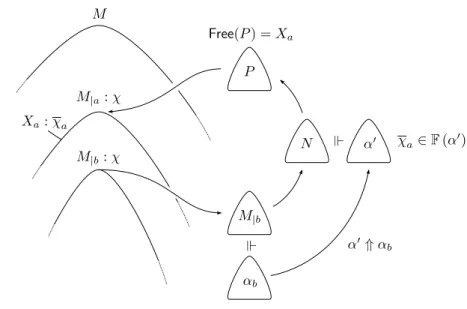
Let us again consider a ΛNF-inhabitant M and two addresses a, b such that a < b, M|a
and M|bare applications of the same type or abstractions of the same type. Suppose:
—there exists a vertical compression α′ of the blueprint of M
|b such that the sequence
Ω(Free(M|a)) can be extracted from α′.
This situation is a generalisation of the last example in the introduction of Section 2 (in which α′ was equal to the blueprint of M
|b, thereby a trivial compression of this
blueprint). The term M is not minimal. Indeed, the key property above implies the existence of a term N of blueprint α′ whose size is not greater than the size of M
|b, and
such that N, M|b, M|aare applications of the same type or abstractions of the same type.
By Lemma 2.16, there exists a term P of the same type and with the same domain as N such that Free(P ) = Free(M|a). The graft of P at a yields an inhabitant of strictly
We will call compact all inhabitants in which the preceding situation does not occur. All inhabitants of minimal size are of course compact. As we shall see in Section 5, we will not need a sharper characterisation of minimal inhabitants. For every formula φ, the set of compact inhabitants of φ is actually a finite set, and our decision method will consist in the exhaustive computation of their domains.
3.1. Depths of the blueprints of minimal inhabitants
Definition 3.1. Two terms M, M′ ∈ ΛNF are of the same kind if and only if they are
both variables, or both applications, or both abstractions, and if they are of the same type.
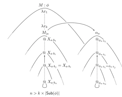
Definition 3.2. For all formulas φ, we write Sub(φ) for the set of all subformulas of φ. Definition 3.3. Let M ∈ ΛNF. Let a be any address in M . Let (a1, . . . , am) be the
strictly increasing sequence of all prefixes of a. Let (λx1, . . . , λxk) be the subsequence
of (M (a1), . . . , M (am)) consisting of all labels of the form λx. We write Λ(M, a) for
(x1, . . . , xk).
Definition 3.4. Let M be a ΛNF-inhabitant of φ. We say that M is locally compact if for
all addresses a in M , the blueprint of M|ais of relative depth at most |Λ(M, a)|×|Sub(φ)|.
Lemma 3.5. Let M be a ΛNF-inhabitant of φ. If M is not locally compact, then there
exist two addresses b, b′ such that b < b′, M
|b and M|b′ are of the same kind and Free(M|b) = Free(M|b′). Moreover, M is not a ΛNF-inhabitant of φ of minimal size.
Proof. For each address a in dom(M ), let αa be the blueprint of M|a and let Xa =
Free(M|a). Assume the existence of an αa of relative depth n > |Λ(M, a)| × |Sub(φ)|. There exist b1, . . . , bn+1∈ dom(αa) such that b1 < . . . < bn < bn+1. By Lemma 2.8.(1)
we have Xa·bn⊆ . . . ⊆ Xa·b1 ⊆ Λ(M, a). By Lemma 1.5, each φa·bi is a subformula of φ. Hence there exist i, j such that i < j and (Xa·bi, φa·bi) = (Xa·bj, φa·bj), that is, M|a·bi and M|a·bj are applications of the same type and with the same free variables (Figure 10). Now, let M′ = M [a · bi← M|a·bj]. The term M
′ is a Λ
NF-inhabitant of φ of strictly
smaller size.
3.2. Vertical compression of a blueprint
Definition 3.6. We let ⇑ be the least reflexive and transitive binary relation on blueprints satisfying the following: if a, b ∈ dom(β), a < b and β(a) = β(b), then β[a ← β|b] ⇑ β.
Lemma 3.7. Suppose M ∈ ΛNF, M : φ, M β and α ⇑ β. There exists a term
M′∈ Λ
NFof the same kind as M , of blueprint α and such that |dom(M′)| ≤ |dom(M )|.
Proof. It suffices to consider the case of α = β[a ← β|b] with a, b ∈ dom(β), a < b and
β(a) = β(b). We prove the existence of M′ by induction on the length of a. If a = ε then
M is necessarily an application and β(ε) = β(b) = @φ, hence M|b is an application of
type φ, and we can take M′= M
Fig. 10. Proof of Lemma 3.5.
(1) Suppose M = (M1M2), M1 β1, M2 β2, a = (i) · aiand b = (i) · bi. By induction
hypothesis there exists M′
i of blueprint αi = βi[ai ← βi|bi] = βi[ai ← β|b], of the same kind as Mi and such that dom(Mi′) ≤ dom(Mi). Let j = 1 if i = 2, otherwise let j = 2.
Let (M′
j, αj) = (Mj, βj). Let X = (x1, . . . , xn) be the strictly increasing sequence of all
variables free or bound in M′
2. Let Y = (y1, . . . , yn) be a strictly increasing sequence of
variables such that Ω(X) = Ω(Y ) and y1is greater that or equal to the greatest variable
of M′
1. Let M2′′ be the term obtained by replacing each xi by yi in M2′. We can take
M′= (M′ 1M2′′).
(2) Suppose M = λx.M1, M1 β1, x : χ, a = (1) · a1and b = (1) · b1. As a, b ∈ dom(β),
we have also a1, b1∈ dom(β1). By induction hypothesis there exists M1′ of the same kind
as M1, of blueprint α1= β1[a1← β1|b1] and such that dom(M
′
1) ≤ dom(M1). By Lemma
2.15.(2.a) there exist γ1, c0, . . . , cpsuch that {c0, . . . , cp} = {c | M|c= x}, β1⊲cχ0. . . ⊲ cp
χ γ1
and β = ∗(γ1). Since a, b ∈ dom(α), a1and ci are incomparable addresses for all i. Hence
α1 = β1[a1 ← β1|b1] ⊲
c0
χ . . . ⊲ cp
χ γ1[a1 ← β1|b1] = β[a ← β|b]|(1) = α|1. By Lemma 2.16
there exists a term M′′
1 of the same type and with the same domain as M1′ such that the
greatest variable y free in M′′
1 is of type χ and {c | M1 |c′′ = y} = {c0, . . . , cp}. By Lemma
2.15.(2.b) we have λy.M′′
1 α, hence we may take M′ = λy.M1′′.
Definition 3.8. A term M ∈ ΛNFis compact when there are no a, b, α′ such that a < b,
M|a and M|bare of the same kind, M|b αb, α′⇑ αb and Ω(Free(M|a)) ∈ F (α′).
Lemma 3.9. Every ΛNF-inhabitant of minimal size is compact. Every compact ΛNF
-inhabitant of φ is locally compact.
Fig. 11. Proof of Lemma 3.9, part (1).
(1) Assume M is not compact. Let a, b be such that a < b, M|a and M|b are of the
same kind, M|b αb, α′ ⇑ αb, Free(M|a) = Xa and Ω(Xa) ∈ F (α′) (see Figure 11). By
Lemma 3.7 there exists a term N ∈ ΛNF of blueprint α′, of the same kind as M|b and
such that |dom(N )| ≤ |dom(M|b)|. By Lemma 2.16 there exists P ∈ ΛNF of blueprint
α′, of the same kind as N , such that dom(P ) = dom(N ) and Free(P ) = X
a. The term
M [a ← P ] is then a ΛNF-inhabitant of φ of smaller size.
(2) Suppose M meets the conditions of Lemma 3.5. Let αb′ be the blueprint of M|b′. By Lemma 2.15.(3) we have Ω(Free(M|b)) = Ω(Free(M|b′) ∈ F (αb′). Since the relation ⇑ is reflexive, M is not compact.
4. Shadows
So far we have isolated two properties shared by all minimal inhabitants (Lemma 3.9). We shall now exploit these properties so as to design a decision method for the inhabitation problem.
In Section 4.1 and 4.2 we show how to associate, with each locally compact inhabitant M of a formula φ, a tree with the same domain as M which we call the shadow of M . At each address a this tree is labelled with a triple of the form (χa, γa, φa) where φa is
the type of M|a, the sequence χa is Ω(Free(M|a)), and γa is a “transversal compression”
of the blueprint αa of M|a (Definitions 4.1 and 4.2). Recall that χa∈ F (αa) (by Lemma
2.15.(3)). The blueprint γacan be seen as a synthesized version of αa of the same relative
depth but of smaller “width”, and such that χa ∈ F (γa) ⊆ F (αa).
Each tree prefix of the shadow of M belongs to a finite set effectively computable from φ and the domain of this prefix. In particular, one can compute all possible values for
its labels, regardless of the full knowledge of M – or even without the knowledge of the existence of M . The key property satisfied by this shadow at every address a is:
—for each γ′ ⇑ γ
a, there exists α′ ⇑ αa such that F (γ′) ⊆ F (α′).
This property is sufficient to detect the non-compactness of M for a pair of addresses (a, b) only from the knowledge of χa, φa, γb, φb and the arity of the nodes at a and b.
Indeed, suppose a < b, φa = φb and the nodes at a, b are of the same arity (1, or 2).
Now, assume:
—there exists γ′ ⇑ γ
b such that χa∈ F (γ′).
Then M|a and M|b are of the same kind and there exists α′ ⇑ αb such that χa =
Ω(Free(M|a)) ∈ F (γ′) ⊆ F (α′), therefore M is not compact.
In Section 4.2, what we call a shadow is merely a tree a 7→ (χa, γa, φa) of a certain
shape, no matter if this tree is the shadow of a term or not. This shadow is compact if there is no pair (a, b) as above. Of course, the shadow of a compact term is always compact in this sense.
In Section 5 we will prove that for every formula φ, the set of shadows of compact inhabitants of φ is a finite set effectively computable from φ (hence the same property holds for the set of compact inhabitants of φ), and we will deduce from this key property the decidability of type inhabitation for HRM-terms.
4.1. Blueprint equivalence and transversal compression
Definition 4.1. We let ≡ be the least binary relation on blueprints such that: 1 ∅B ≡ ∅B,
2 φ ≡ φ,
3 if α1≡ β1, α2≡ β2, then @φ(α1, α1) ≡ @φ(β1, β2),
4 if |a| = |b| = n and αi≡ βifor each i ∈ [1, . . . , n], then ∗a(α1, . . . , αn) ≡ ∗b(β1, . . . , βn).
In (3), we assume α1, α2, β1, β2 non-empty. In (4), we assume that the elements of each
sequence a, b are pairwise incomparable addresses. As to avoid circularity we assume also a 6= ε or b 6= ε, and αi, βi6= ∅B for at least one i.
To some extent this equivalence allows us to consider blueprints regardless of the exact values of addresses. For instance ∗a(α1, . . . , αn) ≡ ∗(α1, . . . , αn) ≡ ∗(αn, . . . , α1),
also ∗(∗(α, β), γ) ≡ ∗(α, β, γ) ≡ ∗(α, ∗(β, γ)), etc. It is easy to check that α ≡ β implies F(α) = F (β) – this property will be used without reference.
Definition 4.2. For each m ∈ N , we let xmbe the least binary relation such that:
1 if γ1≡ . . . ≡ γm≡ γm+16≡ ∅B, then ∗a(γ1, . . . , γm) xm∗a·(b)(γ1, . . . , γm, γm+1),
2 if α = ∗a(α1, . . . , αn), β = ∗b(β1, . . . , βp) and α xmβ, then:
(a) @φ(α, γ) xm@φ(β, γ),
(b) @φ(γ, α) xm@φ(γ, β),
(c) ∗a·(c)(α1, . . . , αn, γ) xm∗b·(c)(β1, . . . , βp, γ).
We call m-compression of β every α such that α xmβ. The width of β is defined as the
Again the elements of a · (b), a · (c) and b · (c) must be pairwise incomparable addresses, and α, β, γ must be non-empty. Note that for all non-empty β, we have ∅B x0β, hence
the empty blueprint is the only blueprint of null width. If β is of width m > 0, then for all addresses a, for β|a = ∗a(γ1, . . . , γk) and for each γi 6= ∅B, the sequence (γ1, . . . , γk)
contains no more than m blueprints ≡-equivalent to γi. For instance, if φ, ψ, χ are distinct
formulas, ∗(φ, φ, φ, ψ, ψ, χ) is of width 3, ∗(ω, @ω(∗(φ, ψ), φ), @ω(∗(ψ, φ), φ)) is of width
2, etc.
Definition 4.3. For each m ∈ N , we write ⊑m for the reflexive and transitive closure
of the union of ≡ and xm. We let ⊑maxm denote the subset of the relation ⊑mof all pairs
with a left-hand-side of width at most m. For instance, if φ, ψ, χ are distinct formulas:
∅B ⊑max0 ∗(ψ, χ, φ) ⊑max1 ∗(χ, φ, φ, ψ, ψ) ⊑max2 ∗(φ, φ, φ, ψ, ψ, χ)
Of course α ⊑m β implies α ⊑j β for all j ∈ [1, . . . , m] and clearly, α xm β implies
|dom(α)| < |dom(β)|, therefore xmis well-founded.
Definition 4.4. For all S ⊆ S, for all d ∈ N and for all m ∈ N :
—we let B(S, d, ∞) be the set of S-blueprints of relative depth at most d, —we let B(S, d, m) be the set of all blueprints in B(S, d, ∞) of width at most m. Lemma 4.5. For all finite S ⊆ S, for all d ∈ N and for all m ∈ N :
1 The set B(S, d, m)/≡ is a finite set.
2 A selector R (S, d, m) for B(S, d, m)/≡ is effectively computable from (S, d, m).
Proof. (1) Let Bε(S, d, m) be the set of all rooted blueprints in B(S, d, m). Assuming
Bε(S, d, m)/≡ is a finite set and a selector Rε(S, d, m) for Bε(S, d, m)/≡ is effectively
computable from (S, d, m), we prove that B(S, d, m)/≡ and Bε(S, d + 1, m)/≡ are finite
sets and show how to compute a selector for each set.
Let (α1, . . . , αk) be an enumeration of Rε(S, d, m). Let Σd be the set of all
func-tions from {1, . . . , k} to {0, . . . , m}. For each β ∈ B(S, d, m) there exist β1, . . . , βn ∈
Bε(S, d, m) and b such that β = ∗b(β1, . . . , βn). We let σβ be the function mapping each
i ∈ {1, . . . , k} to the number of occurrences of an element ≡-equivalent to αi in the
sequence (β1, . . . , βn). Clearly σβ ∈ Σd and furthermore for all β′ ∈ B(S, d, m) we have
β ≡ β′ if and only if σ
β= σβ′, hence B(S, d, m) is a finite set. For each τ ∈ Σd, let ρτ = ∗(α11, . . . , α
τ(1) 1 , . . . , α1k, . . . , α τ(k) k ) where each α j i is equal
to αi. We have ρτ ∈ B(S, d, m) and σ(ρτ) = τ , that is, if τ, τ′ ∈ Σd and τ 6= τ′, then
ρτ6≡ ρτ′. Hence we may define R (S, d, m) as {ρτ| τ ∈ Σd}.
The finiteness of Bε(S, d+1, m)/≡follows immediately from the finiteness of B(S, d, m)
and the fact that if β = @φ(β1, β2) and β′= @ψ(β1′, β′2) are elements of Bε(S, d + 1, m),
then β1, β2, β1′, β2′ are non-empty elements of B(S, d, m) and furthermore β ≡ β′ if and
only if β1≡ β1′ and β2 ≡ β2′. The same property allows us to define Rε(S, d + 1, m) as
the set of all blueprints of the form @φ(γ1, γ2) where @φ ∈ S and each γiis a non-empty
element of R (S, d, m).
empty (hence B(S, d, 0) = {∅B} for all d); if m ∈ N+, then Bε(S, 0, m) is the finite set
of all formulas of S.
4.2. Shadow of a term
Definition 4.6. Let φ be a formula. Let Sφ be the union of Sub(φ) (Definition 3.2) and
the set of all @ψ such that ψ ∈ Sub(φ). For each integer k, for each formula φ, we let
R(φ, k) = R (Sφ, k × |Sub(φ)|, k), where R is the function introduced in Lemma 4.5.(2). Definition 4.7. A shadow is a finite tree in which each node is of arity at most 2 and is labelled with a triple of the form (χ, γ, ψ), where χ is a sequence of formulas, γ is a blueprint and ψ is a formula.
We call φ-shadow every shadow Ξ satisfying the following conditions. We have Ξ(ε) = (ε, ∅B, φ). For each a ∈ dom(Ξ), let ka be the number of b < a such that the node of Ξ
at b is unary, and let (χa, γa, ψa) = Ξ(a). Then:
—χa is a sequence of subformulas of φ of length at most ka,
—γa∈ R(φ, ka),
—χa∈ F (γa)
—ψa is a subformula of φ.
Definition 4.8. Let M be a locally compact ΛNF-inhabitant of φ. For each a ∈ dom(M ):
—let χa = Ω(Free(M|a)),
—let αa be the blueprint of M|a,
—let γa∈ R(φ, |Λ(M, a)|) be such that γa⊑max|Λ(M,a)|αa,
—let φa be the type of M|a.
The tree Ξ mapping each a ∈ dom(M ) to (χa.γa, φa) will be called the shadow of M .
Recall that if M is a locally compact ΛNF-inhabitant of φ, then for each address a in M ,
the blueprint αa of M|ais of relative depth at most |Λ(M, a)| × |Sub(φ)|. Every maximal
|Λ(M, a)|-compression of αa produces a shadow α′a with the same relative depth and of
width at most |Λ(M, a)|, to which some element of R(φ, |Λ(M, a)|) is equivalent, thus the shadow of M is well-defined. Note that the choice of γa is possibly not unique (although
it is, since R is a selector and one can actually prove that γ ⊑max
m α and γ′ ⊑maxm α
implies γ ≡ γ′, but this property is irrelevant to our discussion). We assume that some
γa is chosen for each address a in M .
Obviously the shadow of M satisfies the first, second and fourth conditions in the definition of φ-shadows given above – in the next section, we prove that it satisfies also the third.
4.3. Compact shadows and compact inhabitants
Definition 4.9. A shadow Ξ is compact if and only if there are no a, b such that: a < b, the nodes of Ξ at a, b are of the same arity, Ξ(a) = (χa, γa, ψ), Ξ(b) = (χb, γb, ψ) and
there exists γ′⇑ γ
Fig. 12. A compact inhabitant and its shadow.
Compare this definition with the definition of compactness for term (Definition 3.8). With the help of three auxiliary lemmas, we now prove the key lemma of Section 4: if M is a compact inhabitant – a fortiori locally compact by Lemma 3.9 – then the shadow of M is a compact φ-shadow.
Lemma 4.10. If α ⇑ β ⊑1β′, then there exists α′ such that α ⊑1α′ ⇑ β′.
Proof. (1) An immediate induction on |dom(β′)| shows that if α = β[a ← β |b] and
β ≡ β′, then there exist a′, b′ such that a′ < b′ and α ≡ α′ = β′[a′ ← β′
|b′]. As a consequence, an immediate induction on the length of the derivation of α ⇑ β shows that the lemma holds if β ≡ β′.
(2) Another induction on |dom(β′)| shows that if α ⇑ β x
1 β′, then there exists α′
such that α x1 α′ ⇑ β′. The only non trivial case is α = ∗(a1)(α1), β = ∗(a1)(β1) with α1⇑ β1and β′= ∗(a1,a2)(β1, β2) with β1≡ β2. Since α1⇑ β1≡ β2, by (1) there exists α2 such that α1≡ α2⇑ β2. Hence α = ∗(a1)(α1) x1∗(a1,a2)(α1, α2) ⇑ ∗(a1,a2)(β1, β2) = β
′.
(3) Using (1) and (2), the lemma follows by induction on the length of an arbitrary sequence (β0, . . . , βn) such that β0 = β, βn = β′ and βi−1 ≡ βi or βi−1 x1 βi for each
i ∈ [1, . . . , n].
Lemma 4.11. If α ⊑1β, then F (α) ⊆ F (β).
Proof. By induction on |dom(β)|. Since γ ≡ γ′ implies F (γ) = F (γ′) and |dom(γ)| =
|dom(γ′)|, it suffices to consider the case where α is a 1-compression of β. The case
α = ∗(a1)(α1) and β = ∗(a1,a2)(α1, α2) is clear. The remaining cases follow easily from the induction hypothesis.
Lemma 4.12. If α ⊑mβ, then the set of all elements of F (β) of length at most m is a
subset of F (α).
proposition is trivially true if m = 0. Suppose m > 0. The only non-trivial case is α ≡ ∗a(γ1, . . . , γm) and β ≡ ∗a(γ1, . . . , γm, γm+1) with γi ≡ γ for all i. Let Φ = F (γ).
For each integer k, let Φ(k) = ⊛(Φ
1, . . . , Φk) where Φi = F (γ) for each i. Let φ =
(φ1, . . . , φp) ∈ F (β) be such that p ≤ m. We have to prove that φ ∈ F (α). For each J ⊆
{1, . . . , p}, let (j1, . . . , jq) be the strictly increasing enumeration of all elements of J and
let f (J) = (φj1, . . . , φjq). We have φ ∈ F (β) = Φ
(m+1), hence there exist J
1, . . . , Jm+1
such that J1∪ . . . ∪ Jm+1 = {1, . . . , p}, and f (Ji) ∈ F (γ) for each i ∈ {1, . . . , m + 1}.
For each j ∈ {1, . . . , p}, let kj be any element of {1, . . . , m + 1} such that j ∈ Jkj. Then Jk1∪ . . . ∪ Jkp = {1, . . . , p}, so φ ∈ ⊛({f (Jk1)}, . . . , {f (Jkp)}) ⊆ Φ
(p) ⊆ Φ(m)= F (α).
Lemma 4.13. Let M be a locally compact ΛNF-inhabitant of φ. The shadow of M is a
φ-shadow. If M is compact, then this shadow is also compact.
Proof. For each address a in M , the sequence χa = Ω(Free(M|a)) is a subsequence
of Ω(Λ(M, a)), hence the first proposition follows from the definition of the shadow of M , Lemma 1.5, Lemma 2.15.(3) and Lemma 4.12. Let Ξ be shadow of M . Assume Ξ is not compact. There exist a, b ∈ dom(Ξ) = dom(M ) such that Ξ(a) = (χa, γa, ψ),
Ξ(b) = (χb, γb, ψ), the nodes at a,b in Ξ are of the same arity, and there exists γ′ ⇑ γb
such that χa∈ F (γ′). We have M
|a, M|b of the same kind. Let αa, αb be the blueprints
of M|a, M|b. Since γb ⊑max|Λ(M,a·b)| αb, we have γ′⇑ γb⊑1αb. By Lemma 4.10 there exists
α′ such that γ′ ⊑
1 α′ ⇑ αb. By Lemma 4.11, we have χa ∈ F (γ′) ⊆ F (α′), hence M is
not compact.
5. Finiteness of the set of compactφ-shadows
Our last aim will be to prove that for each formula φ, the set of all compact φ-shadows is a finite set effectively computable from φ.
In definition 5.1, we introduce a last binary relation ⋐ on blueprints. The key lemma of this section (Lemma 5.14) shows that whenever S ⊂ S is a finite set (in particular when S is the set of all subformulas of φ and all @’s tagged with a subformula of φ), the relation ⋐ is an almost full relation (Bezem, Klop and de Vrijer 2003) on the set of all S-blueprints: for every infinite sequence γ1, γ2, . . . over B(S), there exists i, j such that
i < j and γi⋐γj. This result will be proven with the help of Melli`es’ Axiomatic Kruskal
Theorem (Melli`es 1998). The finiteness of the set of compact φ-shadows follows from this key lemma with the help of K¨onig’s Lemma (Lemma 5.15). The ability to compute these shadows follows directly from their definition.
By Lemma 4.13, a consequence of this result is also the finiteness for each φ of the set of all compact ΛNF-inhabitants of φ, although our decision method is based on the
computation of shadows of compact terms rather than a direct computation of those terms. It is worth mentioning that the proof of Theorem 5.13 is non-constructive and that it gives no information about the complexity of our proof-search method – this question might be itself another open problem.
5.1. Almost full relations and Higman Theorem
Definition 5.1. We let ⋐ be the relation on blueprints defined by α ⋐ β if and only if for all χ ∈ F (α), there exists γ ⇑ β such that χ ∈ F (γ).
Definition 5.2. Let U be an arbitrary set. An almost full relation (AFR) on U is a binary relation ≪ such that for every infinite sequence (ui)i∈N over U, there exist i, j
such that i < j and ui≪ uj.
The main aim of Section 5 will be to prove the last key lemma from which we will easily infer the decidability of ΛNF-inhabitation: for each finite S ⊆ S, the relation ⋐ is an
AFR on B(S). Proposition 5.3.
1 If ≪ and ≪′ are AFRs on U, then ≪ ∩ ≪′ is an AFR on U.
2 Suppose ≪U is an AFR on U and ≪V is an AFR on V. Let ≪U ×V be the relation
defined by (U, V ) ≪U ×V(U′, V′) if and only if U ≪UU′ and V ≪V V′. Then ≪U ×V
is an AFR on U × V.
Proof. See (Melli`es 1998). Both results appear in the proof of Theorem 1, Step 4 (p.523) as a corollary of Lemma 4 (p.520)
Definition 5.4. Let U be a set, let ≪ be a binary relation. We let S(U) denote the set of all finite sequences over U. The relation ≪S induced by ≪ on S(U) is defined by
(U1, . . . , Un) ≪S (V1, . . . , Vm) if and only if there exists a strictly monotone function
η : {1, . . . , n} → {1, . . . , m} such that Ui≪ Vη(i) for each i ∈ {1, . . . , n}.
Theorem 5.5. (Higman) If ≪ is an AFR on U, then ≪S is an AFR on S(U).
Proof. See (Higman 1952; Kruskal 1972; Melli`es 1998).
5.2. From rooted to unrooted blueprints
Melli`es’ Axiomatic Kruskal Theorem allows one to conclude that a relation is an AFR (a “well binary relation” in (Melli`es 1998)) as long as it satisfies a set of five properties or “axioms” (six in the original version of the theorem – see the remarks of Melli`es at the end of its proof explaining why five axioms suffice). The details of those axioms will be given in Section 5.3.
Four of those five axioms are relatively easy to check. The remaining axiom is more problematical. This rather technical section is entirely devoted to the proof of Lemma 5.11, which will ensure that this last axiom is satisfied. We want to prove the following proposition:
LetS be a finite subset of S. Let Bε be a subset of Bε(S).
LetB = {∗a(β1, . . . , βn)| ∀i ∈ [1, . . . , n], βi∈ Bε}.
If ⋐ is an AFR onBε, then ⋐ is an AFR onB.
extend the property that ⋐ is an AFR on a given set of rooted blueprints to the set all blueprints that have those rooted blueprints at their minimal addresses.
Higman Theorem suffices to show that ⋐S (Definition 5.4) is an AFR on the set of
finite sequences over Bε. However, if one considers an infinite sequence (βi)i∈N over B and
transforms each βi = ∗ai(β i 1, . . . , βnii) where β i 1, . . . , βnii ∈ Bε into σ(βi) = (β i 1, . . . , βnii), the theorem will only provide two integers i, j and strictly monotone function η such that i < j and βi
k ⋐ β j
η(k) for each k ∈ {1, . . . , ni}. This is sufficient to ensure that
βi= ∗ai(β i 1, . . . , βnii) ⋐ ∗b(β j η(1), . . . , β j
η(ni)), but not in general βi⋐βj.
To bypass this difficulty we show how for each blueprint β ∈ B(S), one can extract from the set of all vertical compressions of β a complete set of “followers” of β of minimal size (Lemma 5.7). This set {α1, . . . , αp} has the property that for each φ ∈ F (β), there
exists at least one αi such that F (αi) contains a subsequence of φ – but not necessarily
φ itself. The relative depth of each αi does not depend on the relative depth on β, but
only on S: it is at most Σ1+|S@|
i=1 i, where S@ is the set of all binary symbols in S. The
lemma in proven in four steps.
First, observe that the set of all α ⇑ β of relative depth at most Σ1+|S@|
i=1 i is a complete
set of followers. If we consider the set of all γ such that γ ⊑max
1 α for at least one such
α, we obtain a (possibly infinite) set closed under ≡ and finite up to ≡. We call it the set of S-residuals of β.
Second, we prove that the set of S-residuals of β is a complete set of followers of β in the same sense, that is, for each φ ∈ F (β) there exists an S-residual γ of β such that F(γ) contains a subsequence of φ (Lemma 5.9).
Third, we prove that if β = ∗a(β1, . . . , βn), β′ = ∗b(β1′, . . . , βn′, β′n+1, . . . , βn+k′ ) are
such that βi ⋐βi′ for each i ∈ [1, . . . , n], and if furthermore β, β′ have the same set of
S-residuals, then β ⋐ β′ (Lemma 5.10).
The last step is the proof of the lemma itself. The set of S-residuals is finite up to ≡ (Lemma 4.5), so there are only a finite number of possible values for the set of residuals of each S-blueprint. As a consequence, it is always possible to extract from an infinite sequence over B an infinite sequence of blueprints with the same set of residuals. The conclusion follows from the third step and Higman Theorem.
Definition 5.6. For every S ⊆ S, we let S@ denote the set of all binary symbols in S.
Lemma 5.7. Let S be a finite subset of S. For all β ∈ B(S), for all ψ ∈ F (β), there exists α of relative depth at most Σ1+|S@|
i=1 i such that α ⇑ β and such that F (α) contains
a subsequence of ψ.
Proof. Call S-linearisation every pair (γ, χ) such that γ ∈ B(S) and χ ∈ F (γ). Call starting address for (γ, χ) every address b for which there exist φ, γ′ such that γ ⊲b
φγ′
and χ ∈ ⊚(F (γ′), (φ)). Call path to b in γ the maximal sequence (b
1, . . . , bn, bn+1) over
dom(γ) such that b1< . . . < bn< bn+1= b.
Given an arbitrary S-linearisation (β, ψ), we prove simultaneously by induction on |dom(β)| the following properties: