The International Temperature Scale: past, present, and future

Publisher’s version / Version de l'éditeur:

Vous avez des questions? Nous pouvons vous aider. Pour communiquer directement avec un auteur, consultez la

première page de la revue dans laquelle son article a été publié afin de trouver ses coordonnées. Si vous n’arrivez pas à les repérer, communiquez avec nous à PublicationsArchive-ArchivesPublications@nrc-cnrc.gc.ca.

Questions? Contact the NRC Publications Archive team at

PublicationsArchive-ArchivesPublications@nrc-cnrc.gc.ca. If you wish to email the authors directly, please see the first page of the publication for their contact information.

https://publications-cnrc.canada.ca/fra/droits

L’accès à ce site Web et l’utilisation de son contenu sont assujettis aux conditions présentées dans le site LISEZ CES CONDITIONS ATTENTIVEMENT AVANT D’UTILISER CE SITE WEB.

NCSLI Measure, 9, 1, pp. 60-67, 2014-03-01

READ THESE TERMS AND CONDITIONS CAREFULLY BEFORE USING THIS WEBSITE. https://nrc-publications.canada.ca/eng/copyright

NRC Publications Archive Record / Notice des Archives des publications du CNRC :

https://nrc-publications.canada.ca/eng/view/object/?id=812eb3f2-deb8-4351-9be1-ec1d66f5db1b https://publications-cnrc.canada.ca/fra/voir/objet/?id=812eb3f2-deb8-4351-9be1-ec1d66f5db1b

NRC Publications Archive

Archives des publications du CNRC

This publication could be one of several versions: author’s original, accepted manuscript or the publisher’s version. / La version de cette publication peut être l’une des suivantes : la version prépublication de l’auteur, la version acceptée du manuscrit ou la version de l’éditeur.

For the publisher’s version, please access the DOI link below./ Pour consulter la version de l’éditeur, utilisez le lien DOI ci-dessous.

https://doi.org/10.1080/19315775.2014.11721675

Access and use of this website and the material on it are subject to the Terms and Conditions set forth at

The International Temperature Scale: past, present, and future Hill, Kenneth D.; Steele, Alan G.

Published in NCSLI Measure J. Meas. Sci., Vol. 9, No. 1, March 2014, pp. 60-67

The International Temperature Scale: Past, Present, and Future

Kenneth D. Hill

ken.hill@nrc-cnrc.gc.ca Alan G. Steele alan.steele@nrc-cnrc.gc.ca National Research Council of Canada

1200 Montreal Road, M-36 Ottawa, Ontario, K1A 0R6

Canada

Abstract: Since its inception in 1927, the International Temperature Scale (ITS) has changed to

meet the needs of the time. The ITS protocol specifies phase transitions with assigned temperatures (the defining fixed points), defining instruments (thermometers), and interpolating (or extrapolating) equations. Since 1927, the selection of fixed points and their assigned temperatures have changed, defining instruments have been added and deleted, and the equations have become more complex.

Since its introduction in 1990, the ITS-90 has served its user community well. However, its departure from thermodynamic temperature is more than is desirable for the most demanding applications. One approach is to continue making measurements on the ITS-90 (T90), and then

correct the temperatures for better accord with thermodynamic temperature (T) using the Consultative Committee for Thermometry’s best estimates of (T – T90). Alternatively, these

shortcomings can be addressed by an evolutionary change that maintains the familiar mathematical structure of the ITS-90, but updates the coefficients of the reference functions and the temperatures of the defining fixed points. The impact on embedded instrumentation is minimal – requiring only an updating of the coefficients of the reference functions and not a complete reworking of the mathematics.

1. Introduction

So you want to measure temperature. What does that mean? Nature and the laws of physics behave according to what is variously referred to as true temperature, absolute temperature, or thermodynamic temperature. However, most measurements are made using a practical temperature scale, such as the International Temperature Scale (i.e. ITS-90), which approximates thermodynamic temperature but is more reproducible.

The ITS protocol is a recipe to construct a temperature scale by specifying the defining fixed points (phase transitions with assigned temperatures), the defining instruments (thermometers), and the interpolating (or extrapolating) equations. Since 1927, the selection of fixed points and their assigned temperatures have changed, defining instruments have been added and deleted, and the equations have increased in complexity. The discussion to follow will focus solely on the portion of the ITS for which the platinum resistance thermometer (PRT) is the defining instrument.

2

Current estimates show that the ITS-90 departs from thermodynamic temperature by more than is desirable and also suffers from a slope discontinuity at the triple point of water. These shortcomings can be addressed through an evolutionary change that maintains the mathematical structure of the ITS-90 while updating the reference temperatures of the defining fixed points and the coefficients of the reference functions. This route to ITS-20XX merits consideration due to the relatively modest requirements for its promulgation.

2. History of the International Temperature Scale

The capabilities of the platinum resistance thermometer (PRT) were demonstrated by H. L. Callendar in his 1887 publication “On the Practical Measurement of Temperature: Experiments Made at the Cavendish Laboratory, Cambridge” [1]. In 1899, Callendar published his “Proposals for a Standard Scale of Temperature based on the Platinum Resistance Thermometer” [2]. The proposed interpolation formula was a quadratic equation in temperature with three calibration points: the melting point of ice (0 °C), the normal boiling point of water (100 °C), and the normal boiling point of sulfur (444.53 °C). Quinn [3] and Hall [4] give accounts of the events following Callendar’s proposal that led to the adoption of the International Temperature Scale (ITS) in 1927 by the Seventh General Conference on Weights and Measures (CGPM). An English version of the text of the ITS-27 was published by Burgess [5] in 1928 in the Bureau of

Standards Journal of Research. From 0 °C to 660 °C, ITS-27 is nearly identical to Callendar’s

proposal: the form of the equation is a quadratic with coefficients determined from calibration at the ice point (0 °C), boiling point of water (100 °C), and boiling point of sulfur (440.60 °C, not the value proposed by Callendar),

Rt = R0 (1 + At + Bt2 ) . (1)

Temperatures from -190 °C to 0 °C are determined from an equation proposed by Van Dusen in 1925 [6],

Rt = R0 [1 + At + Bt2 + C (t – 100) t3 ] . (2)

The coefficient of the cubic term is determined from calibration at the boiling point of oxygen (–182.97 °C).

The Consultative Committee for Thermometry (CCT) was created in 1937 and met for the first time in 1939. At this meeting, a revision of the ITS-27 was agreed upon but war intervened and the revision could not be approved by the CGPM until 1948. The lower limit of the International Temperature Scale of 1948 (ITS-48) [7-9] was increased to –182.97 °C (the oxygen boiling point) because the extrapolation proved to be unreliable. The upper limit of the PRT-defined portion of the scale was reduced from 660 °C to 630.5 °C (freezing point of antimony). The interpolation equations and temperature assignments of the fixed points (oxygen, ice, steam, and sulfur) remained the same. The purity of the platinum was further restricted (R100 / R0 >

1.3910; for ITS-27, the requirement was R100 / R0 > 1.390). The “degree Celsius” replaced

3

With the International Practical Temperature Scale of 1948, Amended Edition of 1960 (IPTS-48) [10], the triple point of water replaced the ice point and the zinc freezing point (419.505 °C) became a recommended alternative to the sulfur boiling point (which remained a defining fixed point). The purity required for the platinum wire was increased once again, the limiting criterion being R100 / R0 > 1.3920.

Though the ITS had remained largely unchanged in form and value for more than 40 years, that familiar circumstance ended with the introduction of the International Practical Temperature Scale of 1968 (IPTS-68) [11,12]. During the 1960s, it was recognized that the ITS needed to be extended to lower temperatures and better accord with thermodynamic temperature was desired [13]. Hall and Barber [14] describe developments from 1948 to 1967 that led to the creation of IPTS-68. Preston-Thomas [15] provides considerable information regarding the context and the process by which the IPTS-68 developed.

Prior to IPTS-68, interpolation from –182.97 °C to 0 °C was based on the Callendar-Van Dusen equation. With IPTS-68, five low-temperature fixed points were added: the equilibrium hydrogen triple point (13.81 K), the equilibrium hydrogen vapor pressure point at 25/76 standard atmosphere (17.042 K), the equilibrium hydrogen boiling point (20.28 K), the neon boiling point (27.102 K), and the oxygen triple point (54.361 K). The temperature T68 is defined by the

relation

W(T68) = WCCT-68(T68) + W(T68), (3)

where W(T68) = R(T68) / R(273.15 K), WCCT-68(T68) is a standard reference function [16], and

W(T68) is a deviation polynomial specific to each sub-range. The sub-ranges are abutting

(13.81 K to 20.28 K, 20.28 K to 54.361 K, 54.361 K to 90.188 K, and 90.188 K to 273.15 K), and the coefficients of the deviation functions for each sub-range are determined by measurements at the defining fixed points appropriate to the specific sub-range and by importing the derivative from the higher-temperature abutting sub-range (except for the 90.188 K to 273.15 K sub-range, which requires the resistance ratio at the water boiling point). Compared to the Callendar-Van Dusen equation, this approach to interpolation must have seemed revolutionary.

Above 0 °C, IPTS-68 retained the customary quadratic equation of Callendar. However, a correction term (“the Moser wobble” [15]) was added to the calculated temperatures in an effort to provide better agreement with thermodynamic temperature. The triple point of water replaced the ice point, the zinc freezing point (419.58 °C) replaced the sulfur boiling point, and the tin freezing point (231.9681 °C) became a permitted alternative to the water boiling point. The purity requirement for the platinum wire increased again, with R100 / R0 > 1.3925 the revised

4

3. The road to the ITS-90

By 1985, a list of the shortcomings of the IPTS-68 had been compiled [17]. The concerns for the PRT portion of the scale were mainly that the IPTS-68 was believed to depart significantly from thermodynamic temperature over much of its range and the non-uniqueness of the low-temperature portion was unnecessarily large due to a poor choice of interpolation function.

With regard to the departure of IPTS-68 from thermodynamic temperature, Working Group 4 (WG4) of the CCT outlined the “Thermodynamic Basis for the ITS-90” in their 1991 publication [18]. The outputs of the WG4 analysis included recommendations for the values of the ITS-90 fixed-point temperatures and a table of (T – T68), their estimate of the differences between the

IPTS-68 and thermodynamic temperature.

As for the matter of the interpolation, Working Group 3 (WG3) of the CCT published “The Platinum Resistance Thermometer Range of the International Temperature Scale of 1990” [19] in 1991 to explain the rationale and process behind the construction of the interpolation function. ITS-90 partitions the PRT range into a low-temperature portion (13.81 K ≤ T90 ≤ 273.16 K) and a

high-temperature range (273.15 K ≤ T90 ≤ 1234.93K). Interpolation requires both a reference

function and a deviation function (W = Wr + W, where Wr represents the reference function and

W is the deviation function). The development of the ITS-90 low-temperature reference

function has been described by Kemp [20]. The construction of the high-temperature reference function was described in detail by Jung [21].

In addition to the reference function, interpolation on the ITS-90 requires appropriate deviation functions to account for the individual behavior of PRTs. The general form of the low-temperature ITS-90 deviation equation is



 



m

 

i n i i W c W b W a W W  



      1 1 ln 1 2 r . (9) The values of m and n are specific to the sub-range, with m being two less than the number of fixed points for the sub-range in question and n a value chosen to minimize the non-uniqueness. The sub-range from 83.8058 K to 273.16 K does not follow this scheme, and instead has as its deviation function

W–Wr = a(W–1) +b(W–1)lnW . (10)

The WG3 publication [19] briefly addresses the development of the high-temperature deviation functions. The full-range form of the equation is

W–Wr = a(W–1) +b(W–1)2+c(W–1)3+d(W-WAl)2 , (11)

with d = 0 below 660.323 °C. In practice, the number of terms depends on the number of fixed points within the sub-range of interest. The complete definition of the ITS-90 may be found in the article by Preston-Thomas [22].

5

4. Is it time to revise the ITS?

ITS-90 has been the consensus standard for more than 20 years, so it is reasonable to ponder whether or not the time is right to revise the scale. Recently, CCT WG4 estimated the extent to which the ITS-90 differs from thermodynamic temperature [23]. From 14 K to 273 K, the maximum difference of 8 mK occurs near 120 °C. Above 273 K, the difference increases with temperature and reaches 29 mK at 660 °C. These differences exceed by a large margin the uncertainties of platinum resistance thermometry at these temperatures, so a case can be made for an updating. Figure 1 indicates how (for the most part) successive revisions have improved the agreement with thermodynamic temperature, and the smoothness of the differences is clearly improving as well.

Figure 1. Differences of the various ITS scales with respect to thermodynamic temperature,

based on WG4’s 2010 estimate of (T–T90) [23].

The slope difference of (T–T90) at 273.16K is another feature seen in Fig. 1. While this was

commented on shortly after ITS-90 came into effect (see for example [24]), it received increased attention when the feature was confirmed by thermodynamic thermometry [25], and recently by analysis of PRT calibrations [26].

A revised ITS should have among its goals: to provide the best possible agreement with thermodynamic temperature, to minimize slope discontinuities for abutting sub-ranges, to minimize non-uniqueness among PRTs within each sub-range, and to minimize the sub-range inconsistency among overlapping sub-ranges. The next question is how to proceed.

-0.10 -0.08 -0.06 -0.04 -0.02 0.00 0.02 0.04 0.06 0.08 0.10 -200 0 200 400 600 Temperature, °C (T T ITS ) , K T48 T68 T90

6

5. A proposal for ITS-20XX

While there are undoubtedly many approaches to designing a temperature scale, the one proposed here maintains the familiar mathematical forms of the ITS-90 (reference and deviation functions), while updating the fixed-point temperatures and the coefficients of the reference functions. The revised temperatures of the defining fixed points can be obtained from the WG4 estimates [23]. Table 1 provides the updated values alongside the ITS-90 assignments.

Fixed Point ITS-90, K ITS-20XX, K

e-H2 triple point 13.8033 13.8037

e-H2 v.p. 17.035 17.0355 e-H2 v.p. 20.27 20.2703 Ne triple point 24.5561 24.5559 O2 triple point 54.3584 54.3573 Ar triple point 83.8058 83.8014 Hg triple point 234.3156 234.3124 H2O triple point. 273.16 273.16 Ga melting point 302.9146 302.919 In freezing point 429.7485 429.7586 Sn freezing point 505.078 505.089 Zn freezing point 692.677 692.691 Al freezing point 933.473 933.502 Ag freezing point 1234.93 1234.976

Table 1. Defining fixed-point temperatures.

To complete the scale definition, the coefficients of the two reference functions and their respective inverse functions need to be provided. For the range 13.8037 K to 273.16 K:

 







XX



i i i XX T A A T W       



 1.5 5 . 1 16 . 273 / ln ln 12 1 0 r , and (12)

 

i XX i i XX T W B B T _        



 0.35 65 . 0 16 . 273 / 6 / 1 r 15 1 0 ; (13) and for the range from 273.15 K to 1234.976 K,

 

XX i i i XX T C C T W         



 481 15 . 754 9 1 0 r , and (14)

7

 

i XX i i XX T W D D T          



 1.64 64 . 2 15 . 273 r 9 1 0 . (15) A0 -2.135 287 07 B0 0.183 321 538 A1 3.183 374 01 B1 0.240 963 636 A2 -1.801 512 31 B2 0.209 062 179 A3 0.716 898 83 B3 0.190 264 326 A4 0.504 644 36 B4 0.142 817 262 A5 -0.618 370 35 B5 0.079 746 736 A6 -0.059 226 32 B6 0.011 405 460 A7 0.279 655 83 B7 -0.042 127 080 A8 0.117 529 88 B8 -0.072 607 348 A9 -0.292 491 31 B9 -0.028 545 314 A10 0.036 398 18 B10 0.074 033 522 A11 0.118 377 63 B11 0.083 379 865 A12 -0.049 991 35 B12 -0.029 391 476 B13 -0.062 007 293 B14 0.001 956 247 B15 0.017 727 617 C0 2.781 502 69 D0 439.951 146 C1 1.646 437 23 D1 472.440 942 C2 -0.137 143 85 D2 37.691 541 C3 -0.006 531 26 D3 7.477 486 C4 -0.002 431 49 D4 2.953 111 C5 0.005 431 32 D5 -0.062 208 C6 0.001 964 53 D6 -1.015 101 C7 -0.002 514 91 D7 -0.072 361 C8 -0.000 457 85 D8 0.209 270 C9 0.000 651 34 D9 -0.004 054

Table 2. The revised constants of the reference functions and the inverse functions.

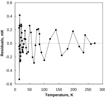
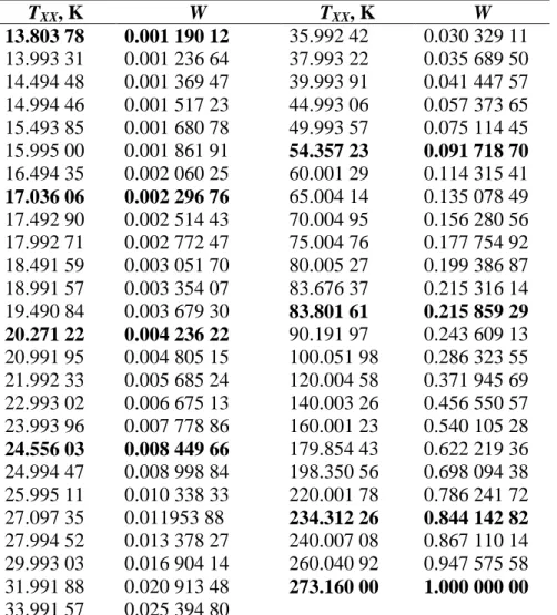
The input data for the low-temperature reference function are in Table 3. The W-values are the same as tabulated by Kemp [20] and the TXX-values are Kemp’s values adjusted by the WG4

estimates for (T–T90) [23]. The fitting residuals appear in Fig. 2 as temperature-equivalents. In

terms of W, the residuals are low in magnitude and well-behaved. However, when expressed in temperature-equivalent (as in Fig. 2), they are slightly higher at the lowest temperatures due to the declining sensitivity of platinum resistivity (Fig. 3).

8

Figure 2. The residuals obtained from fitting the low-temperature reference function.

Figure 3. The sensitivity of platinum resistivity (the first derivative of the low-temperature

reference function) decreases below 90 K and at 14 K is only 6 % of its room-temperature value. -0.6 -0.4 -0.2 0.0 0.2 0.4 0.6 0 50 100 150 200 250 300 Temperature, K Re sidu als , mK 0 0.001 0.002 0.003 0.004 0.005 0 50 100 150 200 250 300 Temperature, K d W r /d T

9 TXX, K W TXX, K W 13.803 78 0.001 190 12 35.992 42 0.030 329 11 13.993 31 0.001 236 64 37.993 22 0.035 689 50 14.494 48 0.001 369 47 39.993 91 0.041 447 57 14.994 46 0.001 517 23 44.993 06 0.057 373 65 15.493 85 0.001 680 78 49.993 57 0.075 114 45 15.995 00 0.001 861 91 54.357 23 0.091 718 70 16.494 35 0.002 060 25 60.001 29 0.114 315 41 17.036 06 0.002 296 76 65.004 14 0.135 078 49 17.492 90 0.002 514 43 70.004 95 0.156 280 56 17.992 71 0.002 772 47 75.004 76 0.177 754 92 18.491 59 0.003 051 70 80.005 27 0.199 386 87 18.991 57 0.003 354 07 83.676 37 0.215 316 14 19.490 84 0.003 679 30 83.801 61 0.215 859 29 20.271 22 0.004 236 22 90.191 97 0.243 609 13 20.991 95 0.004 805 15 100.051 98 0.286 323 55 21.992 33 0.005 685 24 120.004 58 0.371 945 69 22.993 02 0.006 675 13 140.003 26 0.456 550 57 23.993 96 0.007 778 86 160.001 23 0.540 105 28 24.556 03 0.008 449 66 179.854 43 0.622 219 36 24.994 47 0.008 998 84 198.350 56 0.698 094 38 25.995 11 0.010 338 33 220.001 78 0.786 241 72 27.097 35 0.011953 88 234.312 26 0.844 142 82 27.994 52 0.013 378 27 240.007 08 0.867 110 14 29.993 03 0.016 904 14 260.040 92 0.947 575 58 31.991 88 0.020 913 48 273.160 00 1.000 000 00 33.991 57 0.025 394 80

Table 3. The set of (W, T) data on which the low-temperature reference function Wr(TXX) is

based. The bold values identify the defining fixed points.

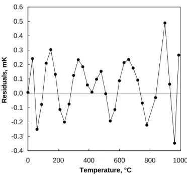
Likewise, the coefficients of the high-temperature reference function can be obtained from the data used by Jung [21]. The W-values in Table 4 are the “smoothed” values of Jung but scaled so that they are in terms of R(t) / R(0.01 °C) rather than R(t) / R(0 °C). The temperatures in Table 4 are those of Jung adjusted by the WG4 estimates of (T–T90) [23]. The fitting residuals

are shown in Fig. 4.

The coefficients of both reference functions (Eqs. (12) and (14)), as obtained by the fitting process described above, are provided in Table 2. For completeness, we also require the coefficients of the inverse functions (Eqs. (13) and (15)). The coefficients of the inverse functions were obtained by fitting 250 (T, W) data pairs obtained by distributing the values of T uniformly over the respective temperature ranges and with the corresponding W values provided by the appropriate reference function.

10

Figure 4. The residuals obtained from fitting the high-temperature reference function.

tXX, °C W tXX, °C W 0.0000 0.999 960 14 480.0187 2.778 143 40 30.0043 1.119 068 97 510.0202 2.880 336 38 60.0077 1.237 089 51 540.0218 2.981 452 81 90.0094 1.354 030 57 570.0234 3.081 483 61 120.0100 1.469 896 98 600.0250 3.180 418 67 150.0100 1.584 693 93 630.5975 3.280 099 07 180.0100 1.698 426 90 660.3245 3.375 916 08 210.0101 1.811 102 14 690.0301 3.470 568 87 240.0103 1.922 725 91 720.1390 3.565 387 78 270.0108 2.033 303 31 750.0336 3.658 418 47 300.0115 2.142 837 84 779.8453 3.750 090 04 330.0123 2.251 331 52 837.0875 3.923 055 08 360.0134 2.358 784 92 898.2316 4.103 444 51 390.0145 2.465 197 04 929.1534 4.192 990 50 420.0158 2.570 564 90 961.8052 4.286 353 20 450.0172 2.674 883 05 988.9654 4.363 104 08

Table 4. The set of (W, T) data on which the high-temperature reference function Wr(TXX) is

based. -0.4 -0.3 -0.2 -0.1 0.0 0.1 0.2 0.3 0.4 0.5 0.6 0 200 400 600 800 1000 Temperature, °C Resi du als , mK

11

6. Testing ITS-20XX

With the reference functions determined, the next task is to test the NRC proposal to ensure that agreement of specific thermometers within the sub-ranges (non-uniqueness) and between overlapping sub-ranges (sub-range inconsistency) are no worse than for the ITS-90. Because the reference functions and deviation functions are nearly the same as those of the ITS-90, the non-uniqueness should be unchanged. Alterations to reference functions and fixed-point temperatures are known to influence sub-range inconsistency, so there is greater need to carry out such tests.

Figure 5 shows the non-uniqueness for the 13.8 K to 273.16 K sub-range using the 35 Ward and Compton [27] thermometers. While other data sets [28] can be used for such testing, the Ward and Compton data have been the most commonly employed for this purpose and are therefore well-suited to evaluating the ITS-20XX formulation. By way of comparison, computation using the ITS-90 reference function and temperature assignments resulted in an identical-looking graph.

Figure 5. Non-uniqueness for the 14 K to 273 K sub-range for the 35 Ward and Compton PRTs

[27]. -1.5 -1.0 -0.5 0.0 0.5 1.0 1.5 0 50 100 150 200 250 300 Temperature, K Non-un iq uenes s, mK

12

Figure 6. Non-uniqueness for the 0 °C to 420 °C sub-range for the 11 Ancsin and Murdock

PRTs [30]. The deviations are expressed with respect to the mean.

Above 273.16 K, PRTs tend to be less stable and comparators with the required stability and isothermality (and also designed to accommodate long-stem PRTs) are rare. Therefore, most of the non-uniqueness estimates are based on measurements of non-defining (secondary) fixed points, such as the freezing point of cadmium. Twenty years ago, the high-temperature non-uniqueness data available at that time was summarized by Hill and Woods [29]. For the present purposes, the data of Ancsin and Murdock [30] at the gallium, indium, bismuth, and cadmium fixed points will be used to assess the non-uniqueness between 0 °C and 420 °C. The result of the analysis appears as Fig. 6. The standard deviations are 0.17 mK, 0.24 mK, 0.29 mK, and 0.42 mK near 30 °C, 157 °C, 271 °C, and 321 °C, respectively. Again, we find no difference in the apparent non-uniqueness between ITS-90 and the NRC ITS-20XX proposal.

The test for sub-range inconsistency requires data for all of the fixed points of the overlapping sub-ranges. Such testing was first described in a document submitted to the 17th meeting of the CCT [31]. For the sub-ranges below 273.16 K, we will use the data reported by Hill and Steele [32]. Figure 7 is the sub-range inconsistency assessment that results from using the ITS-20XX temperature assignments from Table 1 and the ITS-20XX reference function coefficients from Table 2. The extent of sub-range inconsistency is similar to that of the corresponding ITS-90 calculation, but the NRC ITS-20XX proposal is more symmetric about zero, at least for this data set.

-0.6 -0.4 -0.2 0 0.2 0.4 0.6 0.8 1 0 100 200 300 400 Temperature, °C Non -u ni qu en es s, mK

13

Figure 7. Sub-range inconsistency between the 14 K to 273 K sub-range and the 84 K to 273 K

sub-range based on the fixed-point data of Hill and Steele [32].

In a similar manner, we can test the sub-range inconsistency above 273.16 K. For this purpose, we will use the NIST data for six Chino PRTs that was circulated privately by B. W. Mangum [33] to those involved in formulating the ITS-90. When the ITS-90 reference function and fixed-point temperature assignments are employed, the non-uniqueness diagram for this set of PRTs is nearly symmetric about the origin. When the proposed ITS-20XX temperature assignments of Table 1 and the reference function coefficients of Table 2 are used, the non-uniqueness exhibits a negative excursion reaching -1.25 mK. When a zinc fixed-point temperature of 419.5445 °C is used, a sub-range inconsistency diagram is obtained (Fig. 8) with values very similar to the ITS-90 version. This difference of 3.5 mK in the tin fixed-point temperature is significant, but well within the uncertainty of 6.9 mK estimated by WG4 for this temperature. The need to adjust the tin temperature suggests that some “tuning” of the Table 1 assignments may be necessary in order to minimize sub-range inconsistency.

-0.3 -0.2 -0.1 0 0.1 0.2 0.3 0.4 0 50 100 150 200 250 300 Temperature, K Sub -ra ng e in consiste ncy , mK

14

Figure 8. Sub-range inconsistency between the 0 °C to 660 °C sub-range and the 0 °C to 420 °C

sub-range based on fixed-point data from NIST [33]. (Note: this was generated with tXX(Zn) =

419.5445 °C, not the value in Table 1.)

7. Conclusions

The possibility of a revised ITS conforming more closely to thermodynamic temperature than ITS-90 has been demonstrated. Implementation along the lines suggested requires little more than an updating of the coefficients of the reference functions and the temperatures assigned to the defining fixed points. This approach minimizes the need to educate users on the mathematics of the “new” scale, and there is no impact on calibration infrastructure because the ITS-90 fixed points are employed with no additions.

While the ITS-90 design may not be optimal from a mathematical perspective [34], it offers a familiar paradigm that can be updated to improve its accord with thermodynamic temperature. With a clear proposal from NRC in place to bring to fruition ITS-20XX, it is clear that we know how to revise the ITS. Two questions remain to be answered:

1) Should we revise the ITS?

2) If “yes”, then when should the ITS be revised?

Our responses are “Yes” and “Now”. Those who wish to use ITS-20XX will have the authority and guidance to do so and those who prefer to maintain traceability to the ITS-90 are free to choose that course, just as many measurements maintained traceability to the IPTS-68 long after the introduction of the ITS-90.

One potential “driver” for the “yes” and “now” answers is the anticipated change in the definition of the kelvin: when the current triple-point-of-water-based definition is replaced by

-0.4 -0.3 -0.2 -0.1 0 0.1 0.2 0.3 0 100 200 300 400 500 Temperature, °C Sub -ra ng e in consiste ncy , mK

15

one based on fixing the value of the Boltzmann constant, kB. The solution introduced here would

be a natural “mise en pratique” evolutionary solution – an updating of the temperatures of the defining fixed points (including the possibility to introduce others not currently considered as part of ITS-90, such as xenon), and the corresponding interpolating coefficients. This is a graceful and flexible way to accommodate the new knowledge that is likely to come out in the next few years as thermodynamic evaluations (especially at high temperatures) become more commonplace and agreed at the international level.

Updating or revising the ITS in the manner described here should not preclude work on a scale that is better-behaved mathematically. Non-uniqueness from 84 K to 273 K could be reduced by replacing the mercury triple point with the xenon triple point due to its superior positioning (~160 K). This has become feasible with the availability of high-purity xenon and the understanding that isotopic effects do not limit the quality of the xenon triple-point realization [32]. Other improvements should be possible by implementing the suggestions of White [34].

A somewhat longer version of this paper containing additional references and commentary regarding the historical evolution of the ITS appears in the Proceedings of ITS9, the Ninth

International Temperature Symposium held March 19-23, 2012 in Los Angeles, California [35].

8. References

[1] H. Callendar, “On the Practical Measurement of Temperature: Experiments Made at the Cavendish Laboratory, Cambridge,” Phil. T. R. Soc. Lond. A, vol. 178, pp. 161-230, 1887. [2] H. Callendar, “On a practical thermometric standard,” Philos. Mag. Series 5, vol. 48, no. 295,

pp. 519-547, 1899.

[3] T. Quinn, Temperature, Second Edition, London, Academic Press, 1990.

[4] J. Hall, “The Early History of the International Practical Scale of Temperature,” Metrologia, vol. 3, no. 1, pp. 25-28, 1967.

[5] G. Burgess, “The International Temperature Scale,” Bur. Stand. J. Res., vol. 1, no. 4, pp. 635-640, 1928.

[6] M. Van Dusen, “Platinum-Resistance Thermometry at Low Temperatures,” J. Am. Chem.

Soc., vol. 47, pp. 326-332, 1925.

[7] H. Stimson, “The International Temperature Scale of 1948,” Bur. Stand. J. Res., vol. 42, pp. 209-217, 1949.

[8] J. Hall and C. Barber, “The International Temperature Scale – 1948 Revision,” Brit. J. Appl.

16

[9] J. Hall, “The International Scale of Temperature,” in Temperature, Its Measurement and

Control in Science and Industry, vol. 2, edited by H. C. Wolfe, Reinhold Publishing Corp,

New York, NY, pp. 115-139, 1955.

[10] H. Stimson, “International Practical Temperature Scale of 1948- Text revision of 1960,”

Bur. Stand. J. Res., vol. 65A, no. 3, pp. 139-145, 1961.

[11] C. Barber, “The International Practical Temperature Scale of 1968,” Metrologia, vol. 5, no. 2, pp. 35-44, 1969.

[12] C. Barber, “International Practical Temperature Scale of 1968,” Nature, vol. 222, pp. 929-931, 1969.

[13] J. Terrien and H. Preston-Thomas, “Progress in the Definition and in the Measurement of Temperature,” Metrologia, vol. 3, no. 1, pp. 29-31, 1969.

[14] J. Hall and C. Barber, “The Evolution of the International Practical Temperature Scale,”

Metrologia, vol. 3, no. 3, pp. 78-88, 1967.

[15] H. Preston-Thomas, “The Origin and Present Status of the IPTS-68,” in Temperature, Its

Measurement and Control in Science and Industry, vol. 4, edited by H. H. Plumb,

Instrument Science of America, Pittsburgh, pp. 3-14, 1972.

[16] R. Bedford and C. Ma, “A Note on the Reproducibility of the IPTS-68 Below 273.15 K,”

Metrologia, vol. 6, no. 3, pp. 89-94, 1969.

[17] H. Preston-Thomas, T. Quinn, and R. Hudson, “The International Practical Temperature Scale,” Metrologia, vol. 21, no. 2, pp. 75-79, 1985.

[18] R. Rusby, R. Hudson, M. Durieux, J. Schooley, P. Steur, and C. Swenson, “Thermodynamic Basis of the ITS-90,” Metrologia, vol. 28, no. 1, pp. 9-18, 1991.

[19] L. Crovini, H. Jung, R. Kemp, S. Ling, B. Mangum, and H. Sakurai, “The Platinum Resistance Thermometer Range of the International Temperature Scale of 1990,”

Metrologia, vol. 28, no. 4, pp. 317-325, 1991.

[20] R. Kemp, “The Reference Function for Platinum Resistance Thermometer Interpolation between 13.8033 K and 273.16 K in the International Temperature Scale of 1990,”

Metrologia, vol. 28, no. 4, pp. 327-332, 1991.

[21] H. Jung, “The construction of a reference function for platinum resistance thermometers in the range from 0 °C until 962 °C,” Document CCT/89-11, submitted to the 17th Meeting of the CCT, 1989.

[22] H. Preston-Thomas, “The International Temperature Scale of 1990 (ITS-90),” Metrologia, vol. 27, pp. 3-10, 1990. Erratum: Metrologia, vol. 27, p. 107, 1990.

17

[23] J. Fischer, M. de Podesta, K. Hill, M. Moldover, L. Pitre, R. Rusby, P. Steur, O. Tamura, R. White, and L. Wolber, “Present Estimates of the Differences Between Thermodynamic Temperatures and the ITS-90,” Int. J. Thermophys., vol. 32, no. 1-2, pp. 12–25, 2011. [24] K. Hill, “Inconsistency in the ITS-90 and the triple-point of mercury,” Metrologia, vol. 32,

no. 2, pp. 87-94, 1995.

[25] L. Pitre, M. Moldover, and W. Tew, “Acoustic thermometry: new results from 273 K to 77 K and progress towards 4 K,” Metrologia, vol. 43, no. 1, pp. 142–162, 2006.

[26] R. Rusby, “The Discontinuity in the First Derivative of the ITS-90 at the Triple Point of Water,” Int. J. Thermophys., vol. 31, no. 8-9, pp. 1567–1572, 2010.

[27] S. Ward and J. Compton, “Intercomparison of Platinum Resistance Thermometers and T68

Calibrations,” Metrologia, vol. 15, no. 1, pp. 31-46, 1979.

[28] K. Hill and A. Steele, “The Non-Uniqueness of the ITS-90: 13.8033 K to 273.16 K,” in

Temperature, Its Measurement and Control in Science and Industry, vol. 7, edited by D. C.

Ripple, AIP, Melville, NY, pp. 53-58, 2003.

[29] K. Hill and D. Woods, “A preliminary assessment of the non-uniqueness of the ITS-90 in the range 500 °C to 660 °C as measured with a cesium-filled, pressure-controlled, heat-pipe furnace,” in Temperature, Its Measurement and Control in Science and Industry, vol. 6, edited by J. F. Schooley, AIP, Melville, NY, pp. 215-219, 1992..

[30] J. Ancsin and E. Murdock, “An Intercomparison of Platinum Resistance Thermometers Between 0 °C and 630 °C,” Metrologia, vol. 27, no. 4, pp. 201-209, 1990.

[31] K. Hill and R. Bedford, “The minimization of sub-range inconsistency by fixed-point adjustment,” Document CCT/89-6, submitted to the 17th Meeting of the CCT, 1989.

[32] K. Hill and A. Steele, “The triple point of xenon”, Metrologia, vol. 42, no. 4, pp. 278-288, 2005.

[33] B. Mangum, National Institute of Standards and Technology, personal communication, August 1989.

[34] D. White, “Some mathematical properties of the ITS-90,” in Temperature, Its Measurement

and Control in Science and Industry, vol. 8, edited by C. W. Meyer, AIP, Melville, NY, pp.

81-88, 2013.

[35] K. Hill, “An evolutionary approach to updating the International Temperature Scale,” in

Temperature, Its Measurement and Control in Science and Industry, vol. 8, edited by C. W.

18

Appendix A. Request for Feedback from the User Community

The National Metrology Institutes and the Consultative Committee for Thermometry are always interested in hearing from the client community regarding their current and future needs and the potential impact of changes to international consensus standards, such as the ITS.

1) Are you interested in seeing the International Temperature Scale revised for closer accord with “true” thermodynamic temperatures?

2) Would a revision of the ITS along the lines described in this paper meet your needs?

3) Do you think that an updating of instrumentation as proposed (updating the coefficients of the reference functions) offers a practical and cost-effective approach?

4) Can you think of any alternative approaches that ought to be studied by the NMIs?

If you have any feedback for the authors on these or other questions relevant to this paper, we would be pleased to receive your comments by e-mail at ken.hill@nrc-cnrc.gc.ca. Please include the phrase “updating the ITS” in the subject line.

The process to reach agreement on the need and advisability to revise the International Temperature Scale is not simple, but the expert recommendation of the CCT is the usual starting point. The CCT is currently focused on developing a mise en pratique for the kelvin in anticipation of the eventual – but much delayed – redefinition of the kelvin in terms of the Boltzmann constant (which is expected to occur at the same time as the redefinitions of the kilogram, the ampere and the mole). Should support from beyond the NMI community (specifically from industry, instrument manufacturers, and possibly from other stakeholders such as the NCSLI community at large) be garnered for a revision of the ITS, the CCT would either charge Working Group 1 (Defining fixed points and interpolating equations of the ITS-90 and the dissemination of the kelvin) with the responsibility for drafting a suitable proposal (which might follow the NRC approach described here or something similar) or create a Task Force to do so. The approval of any such proposal by the full membership of the CCT would be required to create a formal Recommendation, after which it would be endorsed by the CIPM, and ratified by the CGPM before going into general use. At this time, opinion amongst the NMIs is divided with regard to the merits of revising the ITS: those against such a revision have expressed concern that the potential expense to industry for implementing the change will outweigh the benefits, and they advise continuing the dissemination and use of the ITS-90 indefinitely. Considerable work remains if the CCT is to be persuaded otherwise, and a demonstration of support from the user community will probably be necessary.

View publication stats View publication stats