HAL Id: cirad-01951499
http://hal.cirad.fr/cirad-01951499
Submitted on 11 Dec 2018
HAL is a multi-disciplinary open access
archive for the deposit and dissemination of sci-entific research documents, whether they are pub-lished or not. The documents may come from teaching and research institutions in France or abroad, or from public or private research centers.
L’archive ouverte pluridisciplinaire HAL, est destinée au dépôt et à la diffusion de documents scientifiques de niveau recherche, publiés ou non, émanant des établissements d’enseignement et de recherche français ou étrangers, des laboratoires publics ou privés.
Crop Monitoring Using Vegetation and Thermal Indices
for Yield Estimates: Case Study of a Rainfed Cereal in
Semi-Arid West Africa
Louise Leroux, Christian Baron, Bernardin Zoungrana, Seydou Traore, Danny
Lo Seen, Lo Seen, Agnes Begue
To cite this version:
Louise Leroux, Christian Baron, Bernardin Zoungrana, Seydou Traore, Danny Lo Seen, et al.. Crop Monitoring Using Vegetation and Thermal Indices for Yield Estimates: Case Study of a Rainfed Cereal in Semi-Arid West Africa. IEEE Journal of Selected Topics in Applied Earth Observations and Remote Sensing, IEEE, 2016, 9 (1), pp.347-362. �cirad-01951499�
1 Crop monitoring using vegetation and thermal indices for yield estimates:
1
Case study of a rainfed cereal in semi-arid West Africa 2
3
Leroux La,b*., Baron Ca., Zoungrana Bc., Traoré S.Bc., Lo Seen Da., Bégué Aa. 4
a
CIRAD UMR TETIS, Maison de la Télédétection, 500 rue Jean François Breton, Montpellier, 34093, 5
France 6
b
AgroParisTech, 648 rue Jean François Breton, Montpellier, 34093, France 7
c
AGRHYMET Regional Center, BP 11011, Niamey, Niger 8
*
Corresponding author at: CIRAD UMR TETIS, Maison de la Télédétection, 500 rue Jean François 9
Breton, Montpellier, 34093, France. Email address: louise.leroux@teledetection.fr (L. Leroux) 10
Abstract
11
For the semi-arid Sahelian region, climate variability is one of the most important risks of food insecurity. 12
Field experimentations as well as crop modelling are helpful tools for the monitoring and the 13
understanding of yields at local scale. However, extrapolation of these methods at a regional scale remains 14
a demanding task. Remote sensing observations appear as a good alternative or addition to existing crop 15
monitoring systems. In this study, a new approach based on the combination of vegetation and thermal 16
indices for rainfed cereal yield assessment in the Sahelian region was investigated. Empirical statistical 17
models were developed between MODIS NDVI and LST variables and the crop model SARRA-H 18
simulated aboveground biomass and harvest index in order to assess each component of the yield 19
equation. The resulting model was successfully applied at the Niamey Square Degree (NSD) site scale 20
with yield estimations close to the official agricultural statistics of Niger for a period of 11 years (2000-21
2011) (r=0.82, pvalue<0.05). The combined NDVI and LST indices based model was found to clearly 22
outperform the model based on NDVI alone (r=0.59, pvalue<0.10). In areas where access to ground 23
measurements is difficult, a simple, robust and timely satellite-based model combining vegetation and 24
2 thermal indices from MODIS and calibrated using crop model outputs, can be pertinent. In particular, such 25
a model can provide an assessment of the year-to-year yield variability shortly after harvest for regions 26
with agronomic and climate characteristics close to those of the NSD study area. 27
28
Keywords: Remote Sensing, Crop yield, NDVI, Land Surface Temperature, Crop model, MODIS, 29
Rainfed cereal, Niger, Harvest Index 30
1. Introduction
31 32
In the Sahelian region of West Africa where traditional rainfed agriculture prevails [1], over 20 33
million people suffered from food insecurity in 2014 [2]. Sahelian rainfed farming systems are known to 34
be at high climatic risk due to a high spatio-temporal variability of rainfall and frequent drought events 35
[3]. Rainfall variability results in large fluctuations in year-to-year crop productivity which leads to 36
episodes of food insecurity. Moreover, the political and socio-economic instability of certain countries in 37
the region also contribute to the variability of agricultural production [4]. These considerations highlight 38
the need for an operational, timely and accurate yield estimation system to assist decision-making [5]–[7]. 39
Yield estimation systems based on crop modelling allow accurate quantitative assessments (e.g. 40
AGRHYMET in West Africa; the AGRI4CAST action in Europe), but are confronted with input data 41
availability and spatial consistency constraints [8], [9]. 42
For more than two decades, Earth Observation systems have been known to play a significant role 43
in vegetation monitoring by providing synoptic, repetitive, timely, objective and cost-effective 44
information on Earth’s surfaces (e.g.[10]–[12]). They have been acknowledged for their valuable 45
contribution to spatial and temporal monitoring of global vegetation and thus have been used extensively 46
in many parts of the world for crop condition monitoring and yield forecasting [9], [13]–[18]. Combined 47
or not with rainfall data, satellite data is currently being used in early warning systems to assess crop 48
development conditions during the growing season (e.g. FEWS-NET (Famine Early Warning System 49
3 Network); GIEWS (Global Information and Early Warning System); FOODSEC (Food Security); 50
GEOGLAM (Group on Earth Observation – Global Agricultural Monitoring)), mainly through the 51
production of regularly updated crop growth anomalies’ maps based on the Normalized Difference 52
Vegetation Index (NDVI). These systems benefit from timely and synoptic satellite data which 53
compensate the lack of reliable and homogeneous ground data, but which remain mainly qualitative and 54
do not include crop yield monitoring. 55
The empirical relationship between remote sensing spectral vegetation indices and in situ 56
observations to predict crop yields before harvest has been tested for a long time in many studies (for a 57
review see [19]). The simplest approach involves the regression between observed yields and vegetation 58
indices, either on a specific date or through a time integral of vegetation indices between two dates [20]– 59
[22]. Among the vegetation indices, the NDVI has been widely employed due to its close relationship to 60
several vegetation parameters like the Leaf Area Index (LAI), the fraction of Absorbed Photosynthetically 61
Active Radiation (fAPAR) or the green biomass [23]–[25]. Furthermore, several studies have found a 62
good correlation between NDVI and crop yields in many study sites around the world [13], [15], [16], 63
[26]–[28]. 64
Nonetheless, there are intrinsic limitations that prevent an operational use of vegetation indices to 65
estimate crop yield. Apart from technical limitations such as low spatial and temporal resolution leading to 66
mixed pixels and incomplete crop growth descriptions respectively, the main limitation is the indirect link 67
between yield and spectral data. Since the 1980’s NDVI is known to be a proxy of the aboveground 68
biomass [11], [24], but the ratio between yield and aboveground biomass (referred hereafter as the harvest 69
index, HI) is also known to be highly variable in space and time. [29], [30] showed that biomass 70
production is linearly related to fAPAR for crop with no water stress, while [31] showed that a linear 71
relation between NDVI and fAPAR can be assumed since their functional response to leaf orientation, 72
solar zenith angle and atmospheric optical depth is similar. 73
On the other hand, the harvest index, also known as the reproductive efficiency, is crop-dependent 74
and sensitive to variables that impact the partitioning of the assimilates into grain, such as the genotype, 75
4 temperature and water/nutrients availability ([32]–[34]). In the Sahelian region, HI is strongly dependent 76
on water conditions during the growing period, in particular during the reproductive stage [35]. Crop 77
water conditions can also be derived from remote sensing data, with indices based on the difference 78
between air and surface temperatures, which are useful indicators of water stress for yield estimation. 79
Indeed, since the 1970’s various remote sensing-based studies have shown that final yields can be related 80
to thermal indices [36], [37]. Based on land surface temperature (LST), the Crop Water Stress Index 81
(CWSI) proposed by [38] was found useful for yield estimation and crop assessment (e.g.[39]–[42]). 82
In the framework of current early warning systems for food security, crop yield monitoring would 83
certainly benefit from the consistency in space and time of remote-sensing based crop yield estimations. 84
For this reason, in this study, we investigate the possibility of combining vegetation and thermal indices 85
for crop yield estimation in the Sahelian region, where, to our knowledge, this has not been attempted. Our 86
objective is to build a simple, robust and timely satellite-based model for rainfed cereal yield estimates on 87
the basis that: (i) aboveground biomass can be estimated using NDVI, and that (ii) LST data can provide 88
useful information on the harvest index. Such a model would also provide effective assessments of year-89
to-year yield variability. The study is conducted in the South-West of Niger (the Niamey Square Degree 90
site) where rainfed pearl millet dominates the agricultural landscape, and soils as well as agricultural 91
pratices are relatively homogeneous. We use the SARRA-H (System for Regional Analysis of
Agro-92
Climatic Risks) crop model [43], which has already been validated for pearl millet in the Sudano-Sahelian 93
zone [4], to simulate biomass and the corresponding yield for a period of 11 years (2000-2011), using as 94
input data the rainfall measurements from 28 rain gauges and a meteorological station. We derive the 95
NDVI and the CWSI from MODIS data over the same 11-year period to explore their respective 96
relationship with biomass and the harvest index. The model is then validated using crop statistics data at 97
the scale of the Niger Square Degree site. The proposed approach is finally discussed in the framework of 98
a potential operational yield estimation system that would also include data from the upcoming Sentinel-2 99
sensors. 100
5
2. Material
101
2.1. Overall approach
102
We combine satellite-data with agro-meteorological modeling results to analyze the potential of 103
MODIS derived NDVI and LST time series for pearl millet yield assessment in the Niger Square Degree 104
site. The underlying assumptions of our approach are that: 105
(1) Aboveground biomass can be determined from vegetative indices such as the NDVI [44], 106
(2) Harvest indices can be significantly reduced under water-limited conditions [45] due to crop water 107
stress. Land surface temperature (LST) observations can be used as an indicator of crop water 108
stress [38] and thus be related to the harvest index, 109
(3) The combination of NDVI and LST provides a better estimate of yields than the NDVI on its own 110
in water-limited regions. 111
Fig. 1 summarizes the overall methodology. Empirical statistical relationships are sought (1) between 112
a cropland NDVI integrated over different time periods and aboveground biomass simulated by the crop 113
model SARRA-H, and (2) between a cropland CWSI time series derived from LST data and simulated 114
harvest indices by the same model. Crop yield is equal to aboveground biomass multiplied by harvest
115
index, thus the relationships obtained are then (3) combined into a simple model for pearl millet yield 116
assessment based on vegetation and thermal indices. Ideally, a remote sensing-based approach has to be 117
calibrated with reliable ground-measurement data. For our study area, the ground truth data currently 118
available are mainly based on farmer’s declarative survey and suffer from a lack of consistency both in 119
space and time. Consequently, the choice has been made to use simulated data from SARRA-H crop 120
model to overcome this issue knowing that SARRA-H has been validated for this region [4]. The 121
predictive capacity of the remote sensing-based model is then verified at a regional scale with agricultural 122
statistics. 123
6 124
Figure 1: Flowchart of the approach adopted corresponding to the three stage of the remote sensed based model
125
development.
126
2.2. Study area
127
The study area (12.9° – 13.9°N; 1.6° – 3.1°E, hereafter referred to as the NSD site) which includes the 128
Niamey Square Degree site covers about 18,000 km² and is located in South-West Niger (Fig. 2a). The 129
site is part of the AMMA-CATCH observatory (African Monsoon Multidisciplinary Analysis-Coupling 130
the Tropical Atmosphere and the Hydrological Cycle; http://www.amma-catch.org/) and has been chosen 131
for two reasons: (1) rainfall is considered as the main driver of crop yield [46], and (2) the site is 132
instrumented since the early 90’s including a dense network of rain-gauges which are continuously 133
recording rainfall. 134
7 135
Figure 2: The NSD site (Niger) : a) location of the NSD site (red square) and the five departments considered in the study; b)
136
anomalies of annual rainfall (deviation from the mean between 2000 and 2010); c) mean NDVI annual amplitude between
137
2000 and 2010, and location of the 28 rain gauge (red circles) and meteorological (star) stations.
138
The climate is typically Sahelian. Annual ambient temperatures are high and rainfall distribution 139
is monomodal during June-September. Rainfall is highly variable spatially [47] and temporally [48] with 140
10-22% inter-annual variations between 2000-2010 (Fig. 2b). In addition, despite the small size of the 141
study area (about 160 km x 110 km; Fig. 2c), the regional rainfall pattern shows a high latitudinal gradient 142
from 480 mm/year (north of the study site) to 630 mm/year (south). 143
The production system is rainfed, dominated by pearl millet [4] which is drought-resistant and well 144
adapted to the sandy soils predominant in the study area [49]. It is characterized by low inputs [50] and 145
low yields (generally lower than 700 kg/ha; [49]). 146
8
2.3. Satellite data
147
2.3.1. The MODIS Vegetation Indices product (MOD13Q1)
148
The MODIS Vegetation Indices (VI) product (MOD13Q1 collection 5)was used in this study because 149
of its data consistency, providing spatial and temporal information on vegetation conditions every 16 days 150
at 250-m spatial resolution since 2000 [51]. Even if the MODIS data are pre-processed with the CV-MVC 151
(Constrained view angle-maximum value composites) algorithm, noise still exists in the time series due to 152
cloudiness, sensor problems or Bidirectional Reflectance Distribution Function (BRDF) effects [53]. In 153
consequence, we applied a Savitzky-Golay filter to reduce noise and improve the quality of the NDVI 154
time series towards a more efficient crop yield monitoring [54]. After testing different smoothing 155
parameters, a filter width of 4 and a degree of smoothing polynomial of 6 were retained, which allowed to 156
match the upper envelope of the NDVI time series 157
2.3.2. The MODIS Land Surface Temperature product (MOD11A2)
158
The MODIS LST product (MOD11A2, collection 5) is composed of the average value of daily 1-159
kilometer LSTs under clear sky conditions for an 8-day period [55]. The MODIS LST product was 160
validated with in situ temperature measurements recorded at various places and under various surface and 161
atmospheric conditions [56]. According to [56] the MODIS LST accuracy is better than 1 Kelvin. The 162
LST data has been converted to degrees Celsius. As for the MODIS NDVI data, noisy pixels affected by 163
clouds or other atmospheric disturbances were removed when temperatures were below 0°C and the 164
neighboring values in the time series have been linearly interpolated. 165
2.3.3. The MODIS Land Cover Type product (MCD12Q1)
166
The MODIS LCP (MCD12Q1, version 51) contains the International Geosphere Biosphere Program’s 167
(IGPB) classification, describing 17 land cover classes on a yearly basis at a spatial resolution of 500-m 168
[57], [58].Two classes are related to agriculture: cropland (class number 12) and cropland/natural 169
vegetation mosaic (class number 14). Assuming that cultivated land cover area did not vary considerably 170
during the 10-year period of study, only “consistent” pixels (i.e. pixels classified as cropland for more than 171
six years between 2001 and 2010) were kept as cropland and the rest masked out. This crop mask was 172
9 tested against a land cover map based on Landsat images in 2013 and displayed a user accuracy of 73% 173
and a producer accuracy of 50% for the crop classes (not shown here). Because of its availability at a 174
regional scale, we chose to conduct the analysis with the MODIS LCP to ensure the reproducibility of the 175
methodology elsewhere. In this study, we considered that the resulting cropland was approximately 176
equivalent to the pearl millet cultivated area (since pearl millet represents over 70% of the total 177
agricultural production in the study area; [4], [26]). 178
2.4. Climate data
179
A set of daily rainfall data recorded throughout the period 2000-2010 at 28 rain-gauges 180
(corresponding to 28 villages) distributed across the study area (Fig. 2c) was used. This dataset was 181
provided by the AMMA-CATCH observing system. Other weather data including daily minimum and 182
maximum air temperature, wind speed, solar radiation and minimum and maximum air relative humidity 183
measurements were obtained from a weather station located south of Niamey (Fig. 2c). According to [50], 184
the variability of other meteorological data is very low compared to rainfall in this area, such that only one 185
weather station was considered necessary. 186
2.5. Agricultural statistics
187
Agricultural statistics were used in the validation process of the remotely sensed-based yield model. 188
Pearl millet yield data, collected from ground surveys of major staple crops in Niger, was used. These 189
ground surveys are conducted every year by the Niger Agricultural Statistics service at department level 190
and were therefore available for the 2000 and 2010 period. In this study, yield data for the Kollo 191
department and the four surrounding departments were considered (Fig. 2a). 192
3. Methods
193
3.1. Crop model simulations
194
3.1.1. The SARRA-H crop model
195
SARRA-H V3.3 [43], [50] was used in this study to simulate attainable pearl millet yields under 196
climatic constraint in the NSD site at village level. This model is particularly suited for the analysis of 197
10 climate impacts on cereal growth and yield in dry environments. It is currently used by AGRHYMET for 198
operational agro-meteorological forecasting across West Africa. It simulates attainable yield under water-199
limited conditions taking into account potential and actual evapotranspiration, phenology, potential and 200
water-limited assimilation and biomass partitioning (for more details about the SARRA-H crop model see, 201
http://sarra-h.teledetection.fr). The crop model SARRA-H has been calibrated and validated for local 202
photoperiod sensitive pearl millet cultivars using ground surveys conducted in various location across 203
West Africa such as in Senegal, Burkina Faso, Mali or Niger [4]. The model was found to perform well 204
over West Africa through comparison with FAO statistics [58]–[60] or in comparison with other crop 205
models in the framework of the Agricultural Model Intercomparison and Improvement Project (AgMIP, 206
[61]). 207
3.1.2. Aboveground biomass, harvest index and yield simulations
208
Attainable pearl millet aboveground biomass, harvest index and yield were simulated with the 209
SARRA-H crop model for each of the 28 rainfall stations of the NSD site between 2000 and 2010, 210
according to soil type, rainfall regime and agricultural practices (crop varieties and sowing dates). A total 211
of 1276 simulations were conducted. The range of parameters used for the simulation was derived from 212
previous studies and expert knowledge: 213
Crop varieties: Two local pearl millet photoperiodic cultivars are found at the NSD site; Hainy 214
Kirey (90-120 days cycle duration) and Somno (120-150 days cycle duration). These two 215
photoperiodic varieties are particularly adapted to spatial and temporal variability of the length as 216
well as the onset of the rainy season of the Sahelian zone [1], [59]. In the NSD site pearl millet 217
HK represents among 80% of the crop [60], [61]. Pearl millet aboveground biomass, harvest index 218
and yields were simulated considering neither fertilization nor irrigation. 219
Sowing dates: In Sahelian regions, farmer’s agricultural practices choice is highly determined by 220
the climatic constraints. Farmers generally start sowing photoperiodic millet varieties as soon as 221
possible after the first significant rain, to benefit from the flush of available nitrogen associated 222
with early rains, in spite of a high risk of failure and subsequent need of re-sowing [59], [62]. In 223
11 the model, the beginning of the time window considered for the search of the satisfying conditions 224
for sowing was set on the 1st May, and the sowing date was automatically generated by the model 225
as the day when simulated soil water available for the plant is greater than 10 mm at the end of the 226
day. 227
Soil type: According to the Harmonized World Soil Database [63], 75% of soils in the NSD site 228
are sandy and 25% are sandy clay loam. Since there is no existing data presenting the proportion 229
of each soil type in each of the NSD site’s villages respectively, we assumed the proportions 230
proposed for the whole NSD site as being equivalent to the proportion in each village. Yields, 231
aboveground biomass and harvest index were simulated for these two types of soils, weighted 232
according to these proportions and considering two rooting depths (600 mm and 1800 mm) per 233
type of soil. 234
An example of the aboveground biomass output obtained for Torodi village in 2008 is presented in Fig. 3. 235
236
Figure 3: Example of Somno millet simulated aboveground biomass with the crop model SARRA-H for the village of Torodi in
237
2008. The dark curves represent aboveground biomass for a sandy clay loam soil (thin soil in dashed line and deep soil in solid
238
line), the gray curves represent a sandy soil (thin soil in dashed line and deep soil in solid line) and red curve represent the
239
resulting weighted average.
12
3.2. Relationships between crop model simulations and remote sensing
241
indices for pearl millet
242
3.2.1. Processing of remote sensing indices
243
MODIS NDVI time series
244
In Niger cultivated areas are principally gathered around villages within a distance of less than 10-km 245
[26]. To compare the NDVI with simulated aboveground biomass, NDVI median values within a square 246
of 10-km by 10-km (corresponding to 1600 MODIS pixels) around each village were extracted in order to 247
limit the analysis to areas with the higher density of crop surfaces. The median value was used to represent 248
the average situation while minimizing the effect of pixels with a significant proportion of natural 249
vegetation as can be expected when working with a broad-scale crop mask. Mean values were also not 250
appropriate because the NDVI values were found not to be normally distributed. In this study three NDVI 251
time integrals (cumulative values) were defined (Fig. 4): 252
The rainy season (NDVI_RS) extends from its onset to its retreat. In order to take into 253
consideration the spatial and temporal variability of the length of the rainy season, the onset and 254
retreat of the rainy season was computed for each year and for each village of the NSD site 255
following Sivakumar’s definition [64]. 256
The growing period (NDVI_GP) extends from the onset of the rainy season to the end of 257
September (Fig. 4). The end of the crop growing period corresponds approximatively to the 258
harvesting period which was fixed here to the end of September (270th day of the year) since it 259
generally occurs during September [65]. 260
The productive period (NDVI_PP) of the crop growing period corresponds to phenological stages, 261
such as the reproductive or the first maturing stages, which are especially sensitive to water stress. 262
Consequently, yield loss becomes significant under water stress conditions during these drought-263
sensitive stages. The NDVI between the beginning of August (213th day of the year) and the end 264
of September (including the reproductive and the maturation phases as well as the harvesting 265
period) were used to calculate the NDVI integral during the crop productive period. 266
13 The cropland extent obtained from the MODIS Land Cover Product was used to keep only cropland 267
classified pixels in the NDVI integral calculation which allows minimizing the influence of natural 268
vegetation signals. 269
270
Figure 4: The three NDVI time integrated periods, example of the Kollo village in 2005. NDVI profile (black line) during the
271
season is compared to the simulated aboveground biomass (red line).
272
The Crop Water Stress Index (CWSI)
273
The CWSI, commonly used as a plant stress detection index, is originally based on canopy-air 274
temperature difference and their relation to air vapor pressure deficit. It ranges from 0 (ample water) to 1 275
(maximum stress) [38]. [66] suggest an equivalent approach based only on canopy-air temperature 276
differences. The CWSI used in this study can be expressed as: 277
(1)
278
where is the canopy-temperature from MODIS LST data and is the air temperature measurement 279
from the meteorological AGRHYMET station. Subscripts , and refer to the minimum (non-280
stressed crop), maximum (cover no longer transpiring), and observed canopy-air temperature differences 281
14 respectively, computed for each date within the crop mask over the study area. Since the HI of pearl millet 282
is more sensitive to water stress during the crop productive period of the growing season [35], an integral 283
of CWSI was calculated over the productive period as defined previously (CWSI_PP). 284
3.2.2. Model development for aboveground biomass, HI and yield estimation
285
In Niger, pearl millet is characterized by a LAI generally lower than 2, which suggests that the 286
relationships between NDVI and LAI are below the saturation level explained in [67]. The relationship 287
between simulated aboveground biomass and each of the three NDVI time integrals was modeled with an 288
Ordinary Least Square regression (OLS) through the following expression: 289
(2)
290
where represents the simulated aboveground biomass in year t and village n with the crop 291
model SARRA-H, is the NDVI variable for the same year and village, are the
292
parameters to be estimated and is the error term. An OLS was run at village level for the three NDVI
293
time integrals. 294
As for the aboveground biomass estimation, an OLS regression was applied to derive HI from the CWSI, 295
while the crop model output was used to calibrate the remote sensed based model: 296
(3)
297
where represents the simulated HI in year t and village n with the crop model SARRA-H, 298
is the CWSI variable for the same year and village, are the parameters to be estimated
299
and is the error term. 300
The basic equation to estimate yield, is: 301
15 Thus, by replacing each term of Eq. (4) by Eq. (2) and Eq. (3), the following model for yield estimation 302
can be derived (Eq.5): 303
(5)
4. Results
304
4.1. Crop model simulation results
305
The crop model SARRA-H was run for the 28 villages of the NSD site for a period of 11 years (from 306
2000 to 2010). In these simulations, the mean annual simulated yields at village scale vary from 100 307
kg ha-1 to 1400 kg ha-1 (not shown). The yields are in the same order of magnitude that the ones measured 308
by CIRAD (French agricultural research center for development) and AGRHYMET in the NSD site 309
between 2004 and 2008 (400 to 1100 kg ha-1; [71]). The temporal and spatial variability of the outputs of 310
the simulation protocol are presented in Table 1 and Table 2 respectively. Table 1 shows a general high 311
temporal variability of simulated pearl millet aboveground biomass for the 28 villages with a coefficient 312
of variation (CV) ranging from 31% for Gorou Goussa to 63% for Kollo. Compared to the high year-to-313
year variability of the aboveground biomass, the temporal variability of the simulated yields (CV ranged 314
from 19% to 46% between 2000 and 2010) and harvest indices (CV below 40% and mean HI = 0.29) are 315
moderate. Given the size of the study area, the aboveground biomass, the HI and the yield’s spatial 316
variability could be considered relatively high (CV between 9% and 59% Table 2). The years 2000, 2002, 317
2007 and 2010 are those showing the highest spatial variability between the villages (e.g. 30%, 36%, 30% 318
and 52% respectively, for simulated yields). The analysis of the crop model output during these years (not 319
shown) reveals high water stress conditions at the beginning of the growing period (during the vegetative 320
stage), affecting locally some of the villages and resulting in very low simulated aboveground biomass 321
and yields for those years. We also validate the SARRA-H crop model against agricultural statistics by 322
averaging simulated yield at the NSD site level (Fig.5). The yields are overestimated which is one of the 323
16 main drawbacks of many crop models since they simulate potential yields limited by water supply which 324
could be different from the actual yields attained in the field [72]. 325
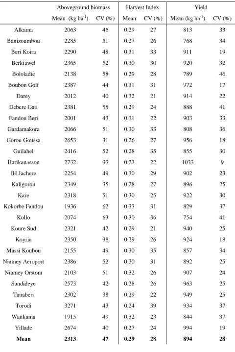
Table 1: Temporal variability of simulated aboveground biomass, harvest index (HI) and yield. The mean values and the
326
coefficients of variation (CV) are calculated on the 2000-2010 period, and are given for each village. In bold, the values
327
averaged of means and CV over the dataset are given.
328
Aboveground biomass Harvest Index Yield
Mean (kg ha-1) CV (%) Mean CV (%) Mean (kg ha-1) CV (%)
Alkama 2063 46 0.29 27 813 33 Banizoumbou 2285 51 0.27 26 768 34 Beri Koira 2290 48 0.31 33 911 19 Berkiawel 2365 52 0.30 30 920 32 Bololadie 2138 58 0.29 28 789 46 Boubon Golf 2387 44 0.31 31 972 17 Darey 2012 40 0.32 21 914 22 Debere Gati 2381 55 0.29 24 888 41 Fandou Beri 2001 43 0.31 22 903 33 Gardamakora 2066 51 0.30 33 808 36 Gorou Goussa 2653 31 0.26 27 956 18 Guilahel 2416 52 0.28 35 855 30 Harikanassou 2732 33 0.27 22 1033 9 IH Jachere 2254 49 0.30 29 902 23 Kaligorou 2349 35 0.28 27 896 25 Kare 2318 51 0.30 25 922 30 Kokorbe Fandou 1936 62 0.33 31 829 37 Kollo 2074 63 0.30 36 754 41 Koure Sud 2321 42 0.29 21 940 25 Koyria 2350 38 0.29 26 924 18 Massi Koubou 2155 49 0.30 35 857 34 Niamey Aeroport 2386 52 0.30 31 892 25 Niamey Orstom 2103 51 0.32 26 907 24 Sandideye 2573 42 0.28 26 963 25 Tanaberi 2302 38 0.29 22 949 25 Torodi 3271 43 0.24 39 934 37 Wankama 1915 49 0.32 23 844 37 Yillade 2674 40 0.27 24 994 19 Mean 2313 47 0.29 28 894 28 329
Table 2: Spatial variability of simulated aboveground biomass, harvest index (HI) and yield. The mean coefficients of variation
330
(CV) are calculated on the 28-village data set, and are for each year. In bold, the values averaged of means and CV over the
331
dataset are given.
332
17
Mean (kg ha-1) CV (%) Mean CV (%) Mean (kg ha-1) CV (%)
2000 2332 24 0.22 21 719 30 2001 2536 23 0.25 23 943 18 2002 1501 52 0.35 15 768 36 2003 3054 24 0.24 17 1050 14 2004 2386 34 0.28 16 949 22 2005 3967 23 0.21 17 1082 12 2006 1706 26 0.36 16 911 15 2007 1989 41 0.31 17 879 30 2008 2781 28 0.27 21 1029 11 2009 2365 41 0.31 24 990 19 2010 828 59 0.43 9 518 52 Mean 2313 34 0.29 18 894 24 333 334
Figure 5: Observed pearl millet yields from agricultural statistics for the department of Kollo vs simulated yields obtained
335
with SARRA-H aggregated at the NSD site level.
336
4.2. Biomass estimation based on NDVI data
337
4.2.1. Results at village scale
338
In order to support the choice of using median values to extract NDVI around each villages, different
339
descriptive statistics have been extracted for each of the NDVI-integrated variables in order to determine
340
the best NDVI-integrated x descriptive statistics combination for aboveground biomass estimation: the
341
median value, the maximum value, the range (the difference between the maximum and the minimum)
342
and the standard deviation. The results are illustrated in Table 3. The four descriptive statistics x the three
343
NDVI-integrated variables were compared to the simulated aboveground biomass using an OLS
18
regression (Table 3). For all the combinations tested the correlation coefficients are low (below 0.40 but
345
all highly significant). The Root Mean Square Errors (RMSE) is high with an RMSE equal to 989 kg ha-1
346
(RRMSE=42%) for the best combination (NDVI median x NDVI_PP), and an RMSE equal to 1060 kg ha
-347
1 (RRMSE=46%) for the less performing combination (NDVI range x NDVI_RS). Fig. 6 shows the
348
resulting scatterplot of NDVI_PP versus simulated aboveground biomass. The dispersion of the points 349
along the regression lines suggests the low ability of MODIS NDVI to reveal spatial and temporal 350
aboveground biomass variability at a village scale. According to the Table 3, the best results are observed
351
for the median NDVI values extracted around villages, thus only the combination NDVI median x
NDVI-352
integrated variables are considered in the remainder of the study.
353
Table 3: Elements of the regression analysis obtained between the simulated aboveground biomass and the descriptive
354
statistics x NDVI variables (NDVI integrated during the rainy season, the growing period and the productive period) obtained
355
at the village scale for years 2000-2010.
356
Descriptive statistics
NDVI
Variables Intercept Slope r p-value RMSE (kg ha-1)
RRMSE (%) Median NDVI_RS 336 0.07 0.32 6.08E-09 1012 43 NDVI_GP 255 0.10 0.34 1.20E-09 1006 43 NDVI_PP -704 0.24 0.38 5.80E-12 989 42 Max NDVI_RS 893 0.03 0.26 5.07E-06 1033 45 NDVI_GP 437 0.06 0.33 5.11E-09 1011 43 NDVI_PP -99 0.13 0.31 1.86E-08 1017 44 Range NDVI_RS 1886 0.01 0.13 0.02 1060 46 NDVI_GP 1585 0.04 0.21 0.0002 1046 45 NDVI_PP 1634 0.06 0.18 0.002 1052 46 Standard Deviation NDVI_RS 1810 0.14 0.16 0.005 1056 45 NDVI_GP 1389 0.34 0.24 3.07E-05 1039 45 NDVI_PP 1280 0.59 0.21 0.0001 1045 45
19 357
Figure 6: Scatterplot of the simulated aboveground biomass (kg ha-1) and the NDVI integrated over the productive period for
358
the 28 villages of the NSD site and over the 11 years of data. The RMSE of the aboveground biomass is 989 kg ha-1 which is
359
equivalent to a RRMSE of 42%, and the correlation coefficient is 0.38. The solid line is the linear regression line and the blue
360
area is the confidence interval for pvalue<0.1.
361
4.2.2. Results at the NSD site scale
362
Since neither NDVI observations nor simulated aboveground biomass follow normal distributions, 363
median values were preferred to mean values to compare NDVI and simulated aboveground biomass over 364
the 28 villages (NSD site scale). The aggregated NDVI value at the NSD site scale was computed
365
considering the NDVI median value for all cropped pixels of the 28 villages. Fig. 7 shows that overall 366
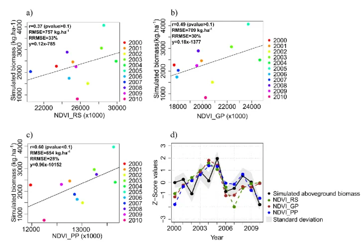
NDVI observations represent well the magnitude of the simulated aboveground biomass variability (Fig. 367
7a, 7b and 7c) as well as the global trends and extreme events (Fig. 7d). Among the three NDVI variables, 368
the NDVI_PP presents the best indicator of pear millet aboveground biomass with a correlation coefficient 369
0.60 (significant at 10%) and a RMSE of 654 kg ha-1 which is equivalent to a RRMSE of 28%, whereas 370
NDVI_RS appears to be the less reliable indicator (Fig 7c and Fig. 7a, respectively). The year-to-year 371
variability is correctly displayed, with a positive trend between 2000 and 2005, a negative trend between 372
2005 and 2010, and NDVI observations differing from simulated aboveground biomass by less than one 373
standard deviation (Fig. 7d). These NDVI trends coincide with the observed rainfall anomalies at the NSD 374
site scale (Fig. 2b). At the site scale, the remote sensing based model for aboveground biomass estimation 375
is expressed as follows: 376
20
(6)
where is the production of pearl millet aboveground biomass estimated at the harvest period in 377
kg ha-1, and _PP is the NDVI integral during the productive period at the NSD site scale. 378
379
Figure 7: SARRA-H simulated aboveground biomass (kg ha-1) vs a) MODIS NDVI integrated during the rainy season, b) MODIS
380
NDVI integrated during the growing season, and c) MODIS NDVI integrated during the productive period. The regression line
381
is in black solid line. d) Comparison of the interannual variability of simulated aboveground biomass and NDVI observations,
382
expressed in z-score values. The grey area is the ± standard deviation computed from simulated aboveground biomass.
383
4.3. Harvest index estimation based of LST data
384
Since aboveground biomass is estimated at the NSD site scale, the model for HI estimation was 385
developed at this same scale by taking the median value of the CWSI_PP derived from the LST data, and 386
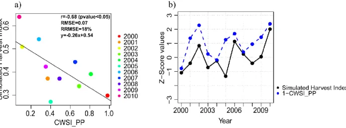
integrated over the crop productive period. The resulting model is presented in Fig.8, which shows that the 387
HI and the CWSI_PP are linearly and negatively correlated, with a correlation coefficient of -0.68
388
(significant at 5%) and a RMSE of 0.07 (Fig.8a). This relationship may be explain by a new biomass 389
21 production allocated to grain decreasing as crop water stress increases, leading to a consequent decrease in 390
yield. In order to better visualize the year-to-year variability of both simulated HI and CWSI_PP, we have 391
plotted the (1-CWSI_PP) value (Fig.8b). The year-to-year variability is generally well represented by the 392
CWSI_PP except for 2005. The model derived for the HI estimation is expressed as follows: 393
(7)
where is the estimated harvest index and is the Crop Water Stress Index’s integrated over 394
the productive period at the NSD site scale. 395
396
Figure 8: a) SARRA-H simulated harvest index vs CWSI_PP estimated from MODIS LST data, over the 2000-2010 period (the
397
regression line is in black solid line); b) comparison of the interannual variability of SARRA-H simulated harvest index and
(1-398
CWSI_PP) values, expressed in z-score values. The grey area is the ± standard deviation computed from simulated harvest
399
index.
400
4.4. Yield estimation based on NDVI and LST data and evaluation
401
Pearl millet yields at the NSD site scale were obtained by multiplying the estimated aboveground 402
biomass (Eq.6; Fig.9a) by the estimated HI (Eq.7; Fig.9b). The estimated yields vary from 390 kg ha-1 to 403
1294 kg ha-1 (Fig.9c). The estimated yields show an overall stable trend between 2000 and 2010 and a 404
decline between 2005 and 2007 (Fig.9c). 405
22 406
Figure 9: Evolution of a) the aboveground biomass estimated from the MODIS NDVI model (Eq. 6), b) the harvest index
407
estimated from the MODIS-derived CWSI model (Eq. 7), and c) the resulting pearl millet yield derived from the combination
408
of Eq. 6 and Eq. 7, over the study site.
409
The predictive capacity of the remote–sensing-based model for pearl millet yield estimation is 410
shown in Fig.10. The combined model based on NDVI and LST data is first evaluated by comparing 411
simulated crop yield (from SARRA-H) to estimates based on the remote sensing-based model (Fig. 10a). 412
The combined model is in moderate agreement with simulated yields (r=0.50, RMSE of 219 kg ha-1 and a
413
Mean Signed Difference [MSD] of 74 kg ha-1; Fig.10a). 414
In order to show the contribution of thermal indices in crop yield estimation, we compared the 415
results with the estimated yields based only on NDVI data. The model (based on both NDVI and LST 416
data) results are in good agreement with the official yield statistics (r=0.82 significant at 5%, Fig.10b). 417
23 Furthermore, the combination of NDVI and LST data clearly contributes to improve yield estimation 418
compared to NDVI data alone (r=0.59, Fig.10c). However, like the crop model used for the calibration, 419
the remote sensing-based models clearly overestimate yields (Fig.10b and Fig.10c) which leads us to
420
consider the ability of these models to render the yield’s year-to-year variability observed by the
421
agricultural statistics. To do so, both estimated and observed yields were normalized. For each year, the
422
absolute differences between agricultural statistics z-score values and those of the models were computed
423
(Fig. 11a). In order to provide an overall indication on the performance of each of the models, the sum of
424
the absolute differences is also assessed. Yield’s year-to-year variability from 2000 to 2010 is quite well
425
rendered in both models in Fig. 11a, particularly for the second half of the period (between 2005 and
426
2010). The combined model based on NDVI and LST data is the closest of the agricultural statistics
427
temporal profile (absolute difference sum = 5.61), particularly in extreme dry years such as in 2000
428
(Fig.11b). Nevertheless, the overall trend is also well transcribed, split in a stable period between 2000
429
and 2005, followed by a decrease trend in yields between 2005 and 2010 (Fig.11b).
430
To test the robustness of the remote sensing-based model, yields for the four surrounding 431
departments were computed and compared with the corresponding official yield statistics (Table 4). 432
Overall, computed yields coincide with the yield statistics, with correlation coefficients above 0.50 433
(significant at 10%) for 3 departments (Table 4). As for the NSD site the remote-sensing based model 434
systematically overestimates yields (RMSE ranging from 237 kg ha-1 to 742 kg ha-1). 435
24 436
Figure 10: a) Simulated yields from SARRA-H vs estimated yields from the combination of NDVI and LST data, and vs
437
estimated yield from remote sensing with (b) or without (c) LST data. The 1:1 line is given in grey dashed line.
438
Figure 11: a) Year-to-year yield variability (SARRA-H, NDVI data, NDVI x LST data) comparison with agricultural statistics. The y-axis indicates the absolute difference between yields anomalies (expressed in z-score) estimated and yield anomalies from agricultural statistics. In brackets are specified the sum of absolute differences. b) Agricultural statistics and simulated yields (NDVI x LST data) standardized anomalies (in z-score).
25
Table 4: Estimated yields from the remote-sensed based model vs the agricultural statistics yields
440 r p-value RMSE (kg ha-1) Fillingue 0.45 0.15 238 Kollo 0.82 0.01 423 Ouallam 0.23 0.48 237 Tera 0.58 0.06 505 Tillaberi 0.64 0.03 742
5.
Discussion
4415.1. Aboveground biomass estimation based on NDVI time series
442
The first stage of the remote sensing-based model consisted in developing an empirical 443
relationship between NDVI time series and pearl millet aboveground biomass simulated by the crop 444
model SARRA-H. 445
The study first highlighted that the ability of the MODIS NDVI time series to estimate 446
aboveground biomass depends on the scale considered. At the village scale (considering the whole dataset: 447
28 villages, 11 years) , the study found out that the MODIS NDVI time series are not able to reveal both 448
the spatial and temporal variability of the simulated aboveground biomass (RRMSE > 40%; Table 3 and 449
Fig.6). As previously shown by [46], in the semi-arid zone of Niamey, aboveground biomass and final 450
yields are mainly influenced by the spatio-temporal distribution of rainfall, and so a high variability of 451
aboveground biomass can be observed between villages which are only a few kilometers apart. Thus, the 452
low correlation between NDVI and aboveground biomass at the village scale implies that the spatial 453
variability of NDVI is not as strongly associated with the spatial variability of rainfall. Further analyses 454
are required on other potential factors that could influence NDVI at this scale. We could assume for 455
instance that, in semi-arid regions where vegetation cover is relatively sparse, soil may cause high 456
variations in the NDVI values at such a small scale, causing NDVI values artifacts [74] and therefore 457
reducing the correlation between NDVI and aboveground biomass. [16], considering a direct relation 458
between NDVI and yield, found that including soil information improved yield prediction in the Peanut 459
Basin in Senegal. On the other hand, at the NSD site scale (temporal analysis), a good correlation was 460
26 found between simulated aboveground biomass and NDVI_PP (r=0.60). This improvement could be 461
explained by (1) the reduction of the noise in the NDVI time series when aggregating at a coarser level 462
and (2) a better representativeness of the overall crop growth conditions over the NSD site that is mainly 463
driven by rainfall variability. 464
The capacity of the MODIS NDVI time series to estimate aboveground biomass depends also on 465
the time period used for the integration. On that point our results are different from [11], [75] who found 466
a good correlation between NDVI integrated over the whole growing season and aboveground biomass in 467
Senegal. In these studies, only natural herbaceous vegetation was considered, for which final aboveground 468
biomass is not much different from vegetative biomass, thus justifying NDVI integration over the entire 469
length of the growing season. Our study focuses on a final aboveground biomass that depends on both 470
vegetative biomass and grains. NDVI values were integrated over the crop productive period to account 471
for grains, since it corresponds to the reproductive period and maturation phases, which include grain 472
filling when plants reach their maximum development [26]. Our results corroborate other studies that 473
directly relate NDVI to yields such as [76] who found that the strongest correlation of NDVI with wheat 474
yields is achieved when taking into consideration NDVI values around their maximum which includes the 475
sensitive stages of grain production.[15] then tested the influence of different NDVI integration periods 476
and found a coefficient of determination R²=0.50 (i.e. r=0.70) for the productive period. In another 477
analysis, using NOAA AVHRR data between 1982 and 1990 for Niger, [26] concluded that the best time 478
integration period for millet and sorghum yield assessment is from August to September. Finally, more 479
recently in a study conducted in China [77] it was also found that the productive and maturing stages 480
including the heading, flowering and filling of the crops are the best suitable periods for yield estimation 481
of paddy rice, corn and winter wheat due to the stress sensitivity of these periods that would lead to 482
biomass reduction and thus potentially yield losses. In our study, NDVI_RS and NDVI_GP (both 483
determined by the onset of the rainy season) appear to be less correlated to aboveground biomass. A 484
potential explanation for this could be the delay between the NDVI onset of the growing season and the 485
calculated start-of-season, which occur one month apart, as previously shown by [78]. At the beginning of 486
27 the growing season in a MODIS pixel the proportion of the millet cover is probably lower than the 487
proportion of the surrounding natural vegetation. The latter reacts immediately to the first significant 488
rainfall, whereas crops are sown later, when sufficient water (>10 mm) is available in the soil [1] and have 489
a growth rate lower than natural vegetation. 490
On the year-to-year variability analysis, a decrease in both the simulated aboveground biomass 491
and the NDVI was observed from 2005 to 2010, with an important decline between 2005 and 2006 (Fig. 492
7d.). When comparing this result with annual rainfall anomalies (Fig. 2b) and it can be concluded that 493
both aboveground biomass and NDVI follow the major trends of rainfall anomalies (as seems particularly 494
evident between 2005 and 2006). This comes in support of the previous assumption that rainfall remains 495
the main determinant of NDVI variability at the NSD site scale. 496
5.2. Harvest index estimation based on an indicator of crop water stress: the
497
CWSI
498
For most crop models, including SARRA-H, DSSAT and CROPWAT [43], [79], [80], water 499
stress during the reproductive and maturation phases is considered a crop yield limiting factor. In the 500
remote-sensing model, we take into account the crop water stress effect on yield through the use of the 501
CWSI, an indicator based on LST. To our knowledge, it is the first time that a link is sought between an 502
indicator of crop stress and HI. An overall good correlation (r=-0.68) was found between HI and 503
CWSI_PP at the NSD site scale, meaning that the HI decreased linearly as the water supply became more 504
limited for plants. However, as for the use of vegetation indices in semi-arid zones, the main issue with 505
thermal indices based on canopy temperature is the spatial heterogeneity due to the soil influence when 506
the canopy does not completely cover the ground. Because bare soil is often much warmer than the air, the 507
soil background temperature included in the LST can lead to false detections of crop water stress [81]. To 508
overcome this limitation, a possibility may be to use the Water Deficit Index developed by [69], which 509
considers both the difference between air and surface temperatures and the fraction of crop cover derived 510
from vegetation indices, to estimate the water status. This method was not tested in this study, as some 511
28 adaptations are ongoing to test the construction of the vegetation index – temperature trapezoid from 512
satellite time series. 513
5.3. Estimation of pearl millet yields
514
The two previous approaches for aboveground biomass and HI estimation were combined into a 515
simple, robust and timely satellite-based model of rainfed cereal yield, applicable at the department level. 516
If in absolute values, yields are overestimated compared to official agricultural statistics of the Kollo
517
department, the analysis of the standardized values has shown a good agreement in terms of year-to-year
518
variability reproduction, translating into a high correlation with statistics. In their recent meta-analysis [8] 519
found that for four studies conducted in Senegal, Burkina Faso and Niger using NOAA AVHRR data, the 520
correlation coefficients between NDVI alone and millet yield were comprised between 0.75 and 0.94
521
which is comparable to the present work (r=0.82). However, caution in the interpretations has to be taken 522
particularly because (1) although the size of the study area considered in these studies is similar to that of 523
the present study (i.e. results aggregated at a department level), the time period considered was much 524
shorter (2 years in[15]) and (2) when the time period considered is comparable to ours, results were 525
aggregated at higher administrative levels than for us (several departments or country level; e.g. [16], 526
[28]). 527
The comparison with a model based only on NDVI has highlighted the usefulness of combining 528
vegetation and thermal indices (NDVI and CWSI) for yield estimation. The ability to render the
year-to-529
year variability of pearl millet yield was clearly improved through this combination, with a correlation
530
coefficient increasing from 0.59 to 0.82 and the z-score absolute difference sum decreasing from 7.28 to
531
6.21. Indeed, because of the spatial variability of management practices, soil water capacity or nitrogen 532
availability, different yields could be observed for the same amount of biomass. In addition, events such as 533
droughts during the reproductive stage, with potentially drastic yield reduction but negligible effects on 534
vegetative biomass, are certainly poorly detected by a model based only on vegetation indices. Thus the 535
direct relation NDVI/yield mostly allows assessing potential harvestable yields when assuming non-536
limiting conditions (i.e. when yield is proportional to aboveground biomass). These potential yields could 537
29 however be reduced by crop water stress during the reproductive stages as shown in this study. 538
Consequently the direct relation NDVI/yield should be considered valid only for specific areas or years 539
without major limiting factors affecting yield. 540
5.4. Limitations of the method
541 542
The remote sensing-based model was applied directly to four surrounding departments and the 543
correlation coefficients were globally good despite an overall tendency to yield overestimation by the 544
model. The four departments are situated at the North of Kollo. They are mainly dominated by 545
agropastoral activities, with a mixture of livestock and crop cultivation [82]. Therefore, the probability to 546
have a mixture of crop vegetation and grasslands within a MODIS cropped pixel is high, which may 547
explain a lower performance of the model. Moreover, in these mixed zones of pasture, the seeding rates 548
are also very low leading to a sparse vegetation cover that causes high NDVI variations due to soil effects. 549
This highlights the main limitation of such models, based on empirical relationships between remote 550
sensing indices and yields: they depend on the environmental characteristics of the study area, which 551
restricts their application elsewhere without recalibration. In addition, such models also depend on the 552
farming system considered. For this reason, the model we developed in this study is only valid for a 553
system based on a single crop and should be tested or adapted for other farming systems such as in the 554
cereal-root crop mixed system where a wide range of different cereals is grown (maize, millet, sorghum or 555
cassava among other) including cases of intercropping. 556
Another consideration to take into account concerning our methodology is the need of a crop 557
mask to isolate cropped pixels. Since a pearl millet crop type map is not available for the NSD site, a crop 558
mask from the MODIS LCP was used here. The same approach was also applied to NDVI and CWSI 559
values extracted from the Landsat Crop mask. A coefficient of correlation of 0.80 is obtained when the 560
resulting estimated yields are compared to official statistics (not shown) which is close to the one obtained 561
with the MODIS LCP product. This confirms the relevance of the approach for the NSD site. However, 562
while the MODIS LCP has been validated for our study area, [83] recently spatialized the uncertainties in 563
30 the localization of cropland in the MODIS LCP over West Africa and showed a high spatial variability 564
with user accuracy varying between 17% to 70% according to farming systems. Thus to extrapolate our 565
methods in other locations, further efforts are needed to develop at least a map locating cultivated zones 566
and if possible the main crop type at a regional scale. 567
The use of a crop model instead of ground measurements to calibrate the remote-sensing model 568
can also be questioned. SARRA-H as most crop models tends to overestimate yields (Fig. 5) since it 569
simulates attainable yields according to agro-meteorological constraints but does not integrate all biotic 570
(e.g. birds, pests, and diseases due to excess moisture) or other non-environmental factors that influence 571
crop management which can lead to yield variations [14], [46], [84] . Remote sensing indices do integrate 572
biotic and non-environmental factors, and because they are calibrated using crop model outputs, an 573
overestimation of yields by the remote sensing-based model could be expected. In addition, since the 574
simulated yields from SARRA-H are overestimated, does that mean that the aboveground biomass and the 575
harvest index are also overestimated? For the latter, the simulated HI as well as the estimated HI are 576
within the range of those measured by [73] over 168 pearl millet plots in the Niamey area. Authors found 577
a mean HI of 0.22, we found a mean simulated and estimated HI of 0.29. For aboveground biomass, 578
reliable measurements in on-farm situations are not available. However, under controlled conditions it has 579
been shown in [46] in Senegal for pearl millet and in [62] for Sorghum in Mali that the aboveground 580
biomass (both yields and growth dynamics) were well simulated by SARRA-H. The same conclusion can 581
be drawn from the study of [4] based on on-farms survey near Niamey (Niger) for pearl millet. 582
Nonetheless, beyond the yields overestimation, our study show that the year-to-year variability is quiet 583
well simulated by the remote sensing based model. 584
Remote sensing indices also present intrinsic limitations. Despite the fact that a filter was applied 585
to reduce noise in the NDVI and LST time series, the presence of clouds, aerosols or dust residues may 586
lead to noise and the downgrading of data quality [85]. Thus, the poor performance of the 587
NDVI/aboveground biomass relation at local scale may also be explained by the 250m x 250m pixel size 588
31 of MODIS images that integrates a mixture of elements (crops, natural vegetation, bare soils) particularly 589
in the semi-arid region with low and sparse vegetation and where crop fields are often smaller than the 590
pixel size. 591
Finally, our study is limited to a period of eleven years and to 28 sites due to the unavailability of 592
more climatic data from ground observations to run the crop model. Agro-meteorological variables 593
derived from satellite could also be considered as an alternative. However, the correct estimation of these 594
variables from satellite, especially rainfall, remains an open issue. For instance, [86] found in the same 595
area that the TRMM 3B42 product, which delivers rainfall estimates at a daily time step, was not able to 596
accurately detect rainfall temporal pattern at the station level, and particularly the intra-seasonal rainfall 597
distribution. We hope that in a few years, the statistical relationships between aboveground biomass and 598
NDVI, and between HI and CWSI, can be updated and made more robust when more climatic data are 599
available. 600
6.
Conclusion and perspectives
601 602
The difficulty to access ground measurements in West Africa and to estimate yields over large 603
areas using other monitoring methods such as agrometeorological modelling makes remote sensing 604
observation a good alternative or addition to consider for early warning systems. In this study, we 605
investigated a new approach based on the combination of vegetation and thermal indices for rainfed cereal 606
yield assessment in the Sahelian region. Empirical statistical models were developed between remote-607
sensing indices (MODIS NDVI and LST), and SARRA-H simulated aboveground biomass and harvest 608
index respectively, and combined for the assessment of crop yield. We demonstrated that the combined 609
model performed better than the one using vegetation index alone. The inclusion of LST improves yield 610
estimations by accounting for the harvest index which is an indicator of the proportion of total 611
aboveground biomass really transformed into grains. In addition, it allows using NDVI as an estimator of 612
aboveground biomass, which is its primary function, rather than an indirect estimator of yield. 613
32 Furthermore, by using a crop model validated over the study area, this study showed that the combination 614
of satellite data with crop modelling is a good option for yield estimation and its year-to-year variability 615
based on remote sensing, especially for areas where ground measurements, required for the calibration of 616
the remote sensing-based model, are not available. 617
Our study confirms that even in small-holder agriculture such as those of the Sahelian region, the 618
use of coarse resolution satellite information for yield monitoring is possible. As the model proposed is 619
simple, robust and based on empirical relations with vegetation and thermal MODIS indices, there is 620
scope for operational implementation of yield estimation at regional scale in a food security early warning 621
system, in particular for the assessment of the year-to-year yield variability in regions with agronomic and 622
climatologic characteristics close to those of the NSD site. In addition, such a system could provide an 623
early estimation of yield shortly after harvest for an area equivalent to an administrative unit unlike 624
agricultural statistics that are currently available from three to six months after harvest. But that would 625
require addressing the issue of multi-crop type systems on which, to the best of our knowledge, no studies 626
have been conducted in the context of the West African farming systems. That would also require the use 627
of a different model for each broad climatic region and each crop type, and their necessary calibration 628
with appropriate ground measurements or crop model simulations. These in turn point out to the need for a 629
better identification of the crop domain and crop types. For instance, upcoming new sensors such as 630
Sentinel-2 (planned launch in June 2015) are expected to significantly improve yield monitoring by 631
providing high spectral, spatial and temporal data, which will allow more regular information on 632
agricultural land use practices. Consequently, a high quality crop type map as well as a stratification map 633
of West Africa according to crop types will become possible and thus the derivation of a remote sensing 634
model calibrated for each crop type. New optical sensors like Sentinel-2 will probably not resolve the 635
problem of data quality loss due to atmospheric effects. Future research must develop improved methods 636
based on the combination of optical and radar data (e.g. Sentinel 2 and 1) to allow vegetation monitoring 637
under all atmospheric conditions. 638


![[DOC] Cours JavaScript : Les Tableaux](data:image/gif;base64,R0lGODlhAQABAIAAAP///wAAACH5BAEAAAAALAAAAAABAAEAAAICRAEAOw==)