Borehole Wave Propagation In Isotropic And Anisotropic Media II: Isotropic Formation

BOREHOLE WAVE PROPAGATION IN ISOTROPIC

AND ANISOTROPIC MEDIA

II: ISOTROPIC FORMATION

by

Ningya Cheng, CoHo Cheng, and MoNo Toksoz Earth Resources Laboratory

Department of Earth, Atmospheric, and Planetary Sciences Massachusetts Institute of Technology

Cambridge, MA 02139

ABSTRACT

In this paper we apply the 3-D finite difference method to simulate borehole wave propagations in an isotropic formation. The scheme is tested in a fluid-filled borehole surrounded by the homogeneous elastic formation. The finite difference synthetics re-sults are in good agreement with the discrete wavenumber solutions for both monopole and dipole sources in hard as well as soft formation. These tests also show the good performance of Higdon's absorbing boundary condition for the body waves as well as the guided waves.

In the isotropic borehole formation, the following results are obtained:

1. Off-centered dipole sources generate almost the same waveforms as the centered dipole source. The slight amplitude differences are due to the different values of the excitation function at the different source positions. The off-centered monopole shows a larger Stoneley wave than the centered one.

2. In an elliptic borehole, where the source is in line with the minor axis of ellipse, the dipole waveforms have similar waveforms to the circular borehole with the same radius as the minor axis. This corresponds to the odd flexural mode. The waveform similarity demonstrates that the odd flexural mode is insensitive to the major axis. When the dipole is in line with the major axis of the ellipse, the waveforms shift to the low frequency range. The waveforms are dominated by the even flexural mode.

44 Cheng et al.

the two flexural modes in the different layers. There are no clear flexural wave reflections in both cases.

INTRODUCTION

Understanding wave propagation around a fluid-filled borehole is essential to acoustic logging data processing and interpretation. The first theoretical work to treat the bore-hole wave propagation problem was done by Biot in 1952. He calculated the borebore-hole guided waves, the pseudo-Rayleigh wave and the Stoneley wave dispersion curves. Pe-terson (1974) analyzed the borehole wave propagation problem by a complex analysis method. The branch cuts and the poles on the complex plane are directly linked to the refracted P and S waves and the guided waves in the borehole.

A number of papers have been published on the synthetic full-waveform acoustic log (White and Zechman, 1968; Rosenbaum, 1974; Tsang and Rader, 1979; Cheng and Toks6z, 1981; Schoenberg et al., 1981; Paillet and White, 1982; Baker, 1984; Tubman et aI., 1984; Schmitt and Bouchon, 1985). The discrete wavenumber technique or a similar one is used to generate these synthetic logs. The centered monopole source (ex-plosion source) and the azimuthal symmetric borehole are considered. Radial layering is allowed. In the early 80's the shear wave logging method was invented to measure the formation shear wave velocity directly, especially in the soft formation (formation shear wave velocity is less than the borehole fluid velocity). The synthetic dipole log also considered the azimuthal symmetric borehole model (Kurkjian and Chang, 1986; Winbow, 1988; Schmitt, 1988). This method works excellently for the simple borehole model which is vertically homogeneous. This allows for the transformation of the ver-tical axis into the wavenumber, then solves the problem in the wavenumber-frequency domain, and is transformed back to the space-time domain. The wavenumber integra-tion is performed numerically and the frequency integraintegra-tion is done by inverse FFT. The boundary element method, combined with the discrete wavenumber technique, is used to treat the vertically irregular borehole (Bouchon and Schmitt, 1989), or the elliptic borehole (Liu and Randall, 1992).

Bhashvanija (1983) and Stephen et al. (1985) applied the finite difference method to the borehole wave propagation in a 2-D cylindrical coordinate. They solve the wave equation in the displacement form by finite difference. The fluid-solid boundary at the borehole wall is treated explicitly to satisfy the boundary conditions, which are the continuity of the normal displacement, stress, and vanishing of the tangential stress. Kostek (1990) applied staggered grid finite difference to the borehole problem in a cylindrical coordinate. The fluid-solid boundary is not treated explicitly because of the staggered grid. Randall et al. (1991) studied monopole and dipole acoustic logs using the staggered grid in a 2-D cylindrical coordinate. They considered an arbitrary azimuthal mode number in the formulation. Randall (1991) also studied the multipole acoustic log in the nonaxisymmetric borehole using the staggered grid finite difference method. In this case the borehole and the formation are assumed invariant in the axial z direction, which allows spatial Fourier transform. The finite difference is performed on a X-Y Cartesian grid. The above methods can be called a 2.5-D finite difference method

3-D Finite Difference II: Isotropic 45

(2-D model plus 3-D source). The only true 3-D finite difference method applied to the borehole acoustic logging was done by Yoon and McMechan (1992). They adopt the second-order staggered grid finite difference scheme.

The reasons for choosing the Cartesian coordinate in this paper to model the bore-hole wave propagation instead of the cylindrical coordinate are the following: First, we are interested in the 3-D structure effect on the acoustic log. These models don't possess azimuthal symmetry, so the cylindrical coordinate doesn't have an advantage. Second, on the 3-D cylindrical grid it is very difficult to treat the point ofr

=

0, and the grid size increases as r becomes large. It is hard to control the grid dispersions. Finally, in the next paper we will consider the borehole wave propagation in an anisotropic formation. The Cartesian coordinate is a generic coordinate to describe the elastic constant tensor. The differences between this paper and the work done by Yoon and McMechan (1992) are the following. First, the accuracy of our scheme is fourth-order and theirs is second order. Our scheme includes anisotropy, a dipole source, a better absorbing boundary condition, and runs on a parallel computer. Second, our staggered grid is arranged differently. Inour arrangement the borehole wall is located where the tangen-tial stress vanishes. Finally, in Yoon and McMechan's paper there isn't any comparison with the known solutions. In this paper we compare our finite difference method with the analytic solutions in the homogeneous acoustic, elastic, and transversely isotropic medium. The finite difference results of the borehole monopole and dipole wave prop-agation are compared with the discrete wavenumber method. Also the finite difference synthetics of the borehole wave propagation in an orthorhombic formation are compared with the ultrasonic lab measurements (see following paper).

In this paper the fourth-order finite difference method is applied to borehole wave propagation in an isotropic formation. The method is further tested in the borehole environment against the discrete wavenumber method for the monopole and dipole sources. More complicated borehole models are considered next. They are for an off-centered tool, an elliptic borehole, and for formation layering.

DISCRETE WAVENUMBER METHOD COMPARISONS

We test the finite difference method for wave propagation in a fluid-filled borehole embedded in an elastic formation in this section. The discrete wavenumber method is a widely used numerical method to compute waveforms in simple borehole geometries (Cheng and Toksiiz 1981; Schmitt 1988). The finite difference results are compared with the discrete wavenumber solutions. This test is unlike those done in the preceeding

46 Cheng et al.

wave has a phase velocity lower than both the formation shear and fluid velocities. Its amplitude decays exponentially on both sides of the fluid-solid boundary. The 8toneley wave is slightly dispersive. The pseudo-Rayleigh wave has phase velocities between the formation shear and fluid velocities. Its amplitude decays exponentially in the forma-tion and is oscillatory in the fluid. The pseudo-Rayleigh wave is highly dispersive and has a cut-off frequency for each mode.

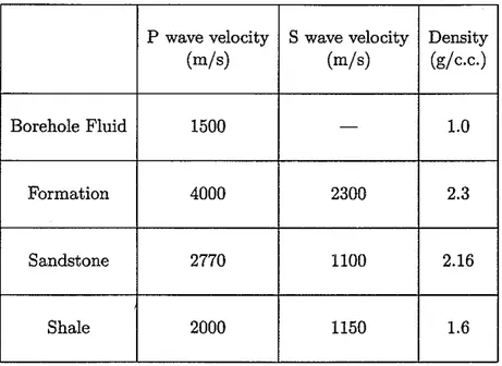
The physical parameters of the borehole fluid and formation are listed in Table 0.1. A grid of 70 x 70 x 200 is used to build the borehole model. The borehole radius is 0.1 m. Because the finite difference grid is in the Cartesian coordinate, the borehole has to be approximated by a rough edged circle. The borehole is numerically drilled along the Z axis.

First the monopole source is considered. The explosion at center frequency 7 kHz is located on the grid at (35, 35, 40), which is the center of the borehole. The source is away from the

z

=

0 because it is the absorbing boundary. Five pressure receivers are located along the borehole center. The distance between the source and the first receiver is 0.7 m and the receiver spacing is 0.2 m. The grid size is 1 cm, which is about

2~

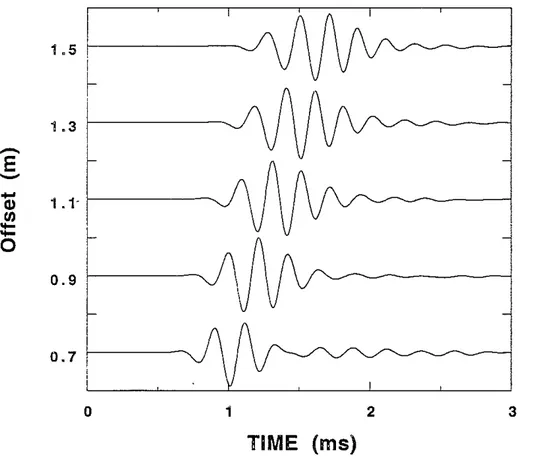
of the fluid P wavelength at the center frequency. The time step is 0.001 ms. The second-order Higdon's absorbing boundary condition is used to reduce the reflections. The local P and 8 wave velocities are substituted into Higdon's formula. Inside the borehole two velocities are set to the fluid velocity. The CPU time for 3000 time step calculations are about 4 hours and 16 minutes with 128 processors.

The comparison of the finite difference synthetics with the discrete wavenumber solutions is plotted in Figure 1. They agree very well. The mismatch reflects the small error of phase difference between the 8toneley wave and the pseudo-Rayleigh wave, which is caused by the grid dispersion. This comparison demonstrates that the staggered grid scheme handles the sharp fluid-solid boundary very well. It also shows that in the inhomogeneous medium Higdon's absorbing boundary condition successfully absorbs the body waves aswell asthe guided waves. The snapshot of the wavefield _rxx at time 0.8 ms is plotted in Figure 2. Most of the wave energy is trapped inside the borehole due to the hard formation (the fluid velocity is less than the formation shear wave velocity). The wavefield is complicated because there are four different kinds of waves present in the borehole. It is hard to identify these waves clearly on the snapshot. To further test the finite difference results we keep all the parameters the same, but increase the source center frequency to 14 kHz. This reduces the grid size to 110 of the fluid P wavelength at the center frequency. The comparison of the finite difference synthetics with the discrete wavenumber solutions is plotted in Figure 3. Once again the agreement is very good. The fourth-order scheme requires fewer grid points per wavelength to get good results. At this frequency range the seismograms are dominated by the pseudo-Rayleigh wave. 80 the mismatch shown in the 7 kHz comparison does not appear here.

In the above test we only considered the hard formation. In the soft formation there is no pseudo-Rayleigh arrivals. The seismograms consist of the leaky P mode and the

3-D Finite Difference II: Isotropic

47

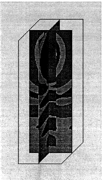
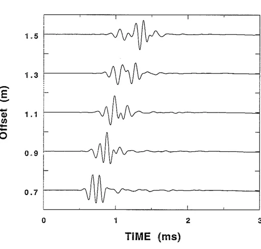
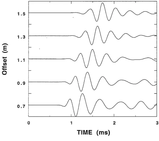
Stoneley wave. The finite difference and the discrete wavenumber comparison is plotted in Figure 4. They are in good agreement. The soft formation parameters are listed in Table 0.1 under entry shale. The grid size and time step as in the previous test is used. The source center frequency is 7 kHz. There are some Stoneley wave amplitude difference between the finite difference syntheics and discrets wavenumber solutions.

Next we consider the dipole source. The dipole is implemented through initiation of the velocity on the source grid. A source with center frequency 3 kHz is located at the borehole center. The dipole direction is along the X axis. All other parameters are the same as the monopole calculation. The receiver records the velocityVx • Comparison of the finite difference results with the discrete wavenumber solutions is shown in Figure 5. The two solutions agree reasonablely well. The flexural mode is a highly dispersive wave. The flexural wave at different frequency travels with a different velocity. The grid dispersion also depends on the frequency. So the different errors are added at different frequencies. Also, in the Cartesian coordinate the borehole near the coordinate axes is approximated by a flat boundary instead of a circular one. The above two reasons explain the discrepancy of the comparison. The wavefield snapshot at time 1.1 ms is shown in Figure 6. Inthe dipole log the wavefields are dominated by the flexural mode so the snapshot is very easy to understand. The image is slightly processed. The zero value of the field is presented by the grey color. It separates the positive and negative part of the fields. The cycles from the seismograms are also reflected on the image. We can also observe from the image that the source radiates waves, then interacts with the formation and sends the flexural mode down the borehole.

The dipole log is invented to measure the formation shear wave velocity directly in the soft formation. Comparison of the finite difference results with the discrete wavenumber solution in the soft formation is shown in Figure 7. The parameters are the same as the soft formation monopole test. The source center frequency is 3 kHz. This comparison is very similar to the hard formation test. The finite difference solution is more dispersive than the discrete wavenumber solution.

OFF-CENTERED SOURCE

In field situations there is no guarantee that the logging tool is always located at the center of the borehole. We have to investigate the off-centered tool effect. Tadeu (1992) and Schmitt (1993) studied the off-centered tool effect by using the discrete wavenumber method. The off-centered tool breaks the azimuthal symmetry, even if the borehole and the formation are azimuthally symmetric. This azimuthal dependence has to be

48 Cheng et al.

Stoneley wave compared with the center source (Figure 1). This can be understood by Stoneley wave amplitude distribution. Its amplitude decays exponentially on both sides of the borehole wall. When the source is moved closer to the borehole wall it will excite Stoneley waves more efficiently.

Off-centered dipole sources are considered next. Figure 10 and Figure 11 show the waveforms of dipole sources applied along the X and the Y directions, respectively. The source positions are the same as the monopole. Figure 10 and Figure 11 display the same waveforms as the centered dipole source (Figure 5). The differences of these plots are the amplitudes. The maximum amplitudes of the centered dipole, the off-centered dipole in the X direction and in the Y direction are 0.01313, 0.01206 and 0.01041, respectively. This can be explained as follows: in the low frequency range, the dipole source excites the dominant flexural mode. These three source positions are capable of exciting the flexural mode but with different efficiency. The snapshot of the wavefield from the off-centered dipole in the X direction at time 1.1 ms is shown in Figure 12. The off-centered source is very clear from the image. Although the image is not exactly as the centered dipole, they share the same characteristics.

In a circular borehole there are two fiexural modes, which have the same phase and group velocities. From a mathematical point of view, the two orthogonal modes are needed to form a complete set. A fiexural wave in any direction can be obtained by a linear superposition of these two modes. Because these two modes are identical in velocity, off-centered dipole sources with different orientations produce the same waveforms. These two modes degraded into one because of the symmetry of the model. In order to split these two modes we have to break the azimuthal symmetry. This leads us to the next section: the elliptic borehole.

ELLIPTIC BOREHOLE

Wells drilled in the earth are often noncircular. This can be caused by tectonic stress, or washout in soft or unconsolidated formations. There are a number of studies of the noncirclar borehole wave propagation problem. Ellefsen (1990) applied the perturbation theory to the normal modes for a slightly irregular borehole. A more complete study of noncircular modes in a fiuid-filled borehole was done by Randall (1991). He used the boundary integral method to solve the problem. This method extended to include an external source for the waveform calculations (Liu and Randall, 1992). Randall (1991) also developed the 2.5-D finite difference technique to compute multipole acoustic wave-forms in nonaxisymmetric borehole and formations. But the borehole and formation are assumed vertically uniform. The finite difference calculations are performed on the horizontal X-Y plane. In this section the 3-D finite difference technique is applied to compute the monopole and the dipole log in an elliptic borehole.

The elliptic borehole, with the minor radius 10 em in the X direction and the major radius 20 em in the Y direction, is embedded in an isotropic formation. The model is illustrated in Figure 13. All other parameters are the same as the test borehole model. First the monopole source at the center frequency 7 kHz is applied at the center of the

3-D Finite Difference II: Isotropic 49

borehole. The pressure receivers are also located at the center of the borehole. The synthetics are plotted in Figure 14. The waveforms in the elliptic borehole are very different from the circular borehole with the 10 cm radius (Figure 1). It is difficult to tell from the waveforms how ellipticity affects the individual wave type. It is more interesting to investigate the ellipticity effect on the dipole log, because it is dominated by the flexural modes. The waveforms from a 3 kHz dipole source in the X and Y directions are plotted in Figure 15 and Figure 16, respectively. The receivers record the velocity in the source's direction. The elliptic borehole breaks the azimuthal symmetry. So it splits the two identical flexural modes into odd and even flexural modes with different phase and group velocities (Randall 1991). For the dipole source applied along the major axis (Figure 16), a very dispersive, low frequency even flexural mode is obtained. The even flexural mode is sensitive to the major radius. The snapshot of the wavefield image (Figure 17) shows the low frequency characteristics very clearly. The wavefield pattern inside of the borehole also matches the pattern of the even flexural mode given by Randall (1991). For the dipole source applied along the minor axis of ellipse (Figure 15), a less dispersive and high frequency odd flexural mode is observed. The odd flexural mode is insensitive to the major radius. The waveforms are similar to the 10 cm circular borehole one (Figure 5). The wavefield image is shown in Figure 18. The wavefields are directed in the minor axis direction.

LAYERING

The crust of the Earth can be approximately described as a stratified medium on the global scale. Locally the geological process tilted these layers or even overturned them. A tilted or even horizontal well Can be drilled in a perfectly horizontal layered crust. In this section we consider the wave propagation in a circular fluid-filled borehole sur-rounded by the layered formation.

Horizontal Bed

Horizontal drilling has become common in the oil industry. Itis interesting to investigate the borehole wave propagation along the borehole which is drilled parallel to a layer boundary. The geometry of this problem is illustrated in Figure 19. The borehole is infinitely long and Figure 19 only shows part of it. The physical parameters of Layer 1 and Layer 2 are listed in Table 0.1 under the entries formation and sandstone. This makes the borehole host layer a slow formation.

50 Cheng et aI.

the leaky P (Figure 21 (b)). It is the refracted P from the bed boundary, because the velocity of Layer 1 is faster than that of Layer 2. This refracted P provides one way to detect the bed near the borehole from the acoustic logging. The 2-D slice of the 3-D wavefield clearly demonstrates the refracted P from the bed boundary (Figure 22). The seismograms from the off-centered tool are plotted in trace (c) for the halfradius (5 cm) away from the bed and (d) for the half radius close to the bed. The waveforms in the trace (c) and (d) are very different from the centered tool. The amplitudes are reduced. When the tool is close to the bed, the refracted P wave smove forward, and when the tool moves away from the bed, the refracted P waves move back. Also the off-centered tool generates a relatively strong Stoneley wave.

Next we investigate the effect of the distance between the borehole center and the bed. The seismograms are plotted in Figure 23. The detailed part of the seisgrams (0 to 1.0 ms) are plotted in Figure 24. The tool is centered inside the borehole. Trace (a) is the one without the bed. Trace (b), (c) and (d) are for the bed away from the borehole center at 10, 20 and 30 cm, respectively. When the bed is tangential to the borehole wall, the waveform is very different and the amplitue is much smaller (Figure 23 (b)). When the bed is moving away from the borehole, the refracted P wave also moves back (Figure 24). This suggests that to detect the structure far away from the borehole the long spacing tool is needed.

Finally, we consider the dipole log. In the dipole log case the properties of Layer 1 and Layer 2 are exchanged. First the dipole source is directed towards the bed. The waveforms are shown in Figure 25. The horizontal bed changed the waveforms dramatically. The amplitude at offset 1.1 m is reduced significantly. This is the shear wave interference caused by the layer boundary. But when the dipole source is directed parallel to the bed (Figure 26), the synthetics are almost the same as the one without the bed. This demonstrates that the dipole is a directional source. Itonly sensitizes to a structure which is in the source's direction.

The wavefield snapshot from the dipole, which is toward the bed, at time 1.

i

ms is plotted in Figure 27. The image is rotated 90 degrees vertically. The borehole wall and the bed boundary can be clearly seen from the snapshot. Because the velocity in Layer 1 is slower than the borehole host layer the wavefronts fall back in Layer 1. The wavefield snapshot from the dipole, which is parallel to the bed, is shown in Figure 28. The layer boundary is not very clearly divided from the image, but that the shear wave in Layer 1 is slower than Layer 2 can still be observed.

Tilted Layers

In logging practice it is also common to encounter the tilted layer. A fluid-IDled borehole penetrating a tilted layer formation is considered. The model is illustrated in Figure 29. The layer boundary intercepts the borehole axis at an angle of 45 degrees. The strike of the layer boundary is parallel to the Y axis. Layer 1 and Layer 2 have the same physical properties as the horizontal bed dipole examples. The borehole radius is 0.1 m. The grid size is 0.01 m and the time step size is 0.001 ms. The whole 3-D grid is 70 x 70 x 300. The source is located at the grid point (35, 35, 40). The layer boundary

3-D Finite Difference II: Isotropic

51

crosses the borehole center at the grid point (35, 35, 200). The receivers are located at the borehole center. The distance of the source and the first receiver is 0.7 m. The receiver spacing is 0.2 m. The layer boundary cross point is at offset 1.6 m.

The synthetic monopole waveforms are plotted in Figure 30. For the purpose of comparison the synthetics from the horizontal layered formation are shown in Figure 31. In the horizontal layered case, the boundary also crosses the borehole center at the grid point (35, 35, 200). The plots demonstrate that the horizontal layered boundary generates a stronger reflection and transmission than the 45 degree tilted boundary. The tilted boundary represents the smooth change of the formation properties. 80 it reduces the reflection and drives more energy away from the borehole to the formation. The tilted boundary also helped the 8 wave to the P wave conversion at the boundary (Figure 30), which is the small first arrival on the seismograms at offset 1.9 to 2.5 m. But this conversion is not shown in the horizontal boundary case. The different incident angles, zero degree at the horizontal boundary and 45 degrees at the tilted boundary, explain the occurrence or absence of these conversions.

In the dipole log, the synthetics of the dipole, which is parallel to the boundary strike (Y axis), are plotted in Figure 32. The synthetics of the dipole, which is perpendicular to the boundary strike, are plotted in Figure 33. The dipole synthetics in the borehole near the horizontal layer boundary are shown in Figure 34. In the horizontal boundary case the transmitted flexural wave in Layer 2 is very clear. The transmitted flexural wave in Layer 2 reflects the fact that the shear wave velocity in Layer 2 is slower than in Layer 1. Transmitted flexural waves across the 45 degree tilted boundary have only about half the amplitude of the one transmitted across the horizontal boundary. There is no clear reflected flexural wave from both boundaries. The 2-D slice wavefield from the dipole in the borehole near the horizontal layer boundary is shown in Figure 35. The flexural wave transmitted through the boundary can be seen (the last cycle). The wavefronts are still flat. The 2-D slice wavefield from the dipole in the borehole near the 45 degree tilted layer boundary is shown in Figure 36. The flexural wave transmitted through the boundary can also be seen (the last cycle), but the wavefronts become tilted about 45 degrees.

CONCLUSION

In this paper a 3-D finite difference method is applied to the borehole wave propagation in an isotropic formation. The finite difference synthetics of the monopole and the dipole log in a fluid-filled borehole are compared with the discrete wavenumber method. They

52 Cheng

et

aI.

P wave velocity S wave velocity Density

(m/s) (m/s) (g/c.c.)

Borehole Fluid 1500 - _1.0

Formation 4000 2300 2.3

Sandstone 2770 1100 2.16

Shale 2000 1150 1.6

Table 1: Borehole model parameters

In the elliptic borehole, two flexural modes are split. The dipole source, directed along the minor axis, excites the odd flexural mode, which is insensitive to the major radius. The dipole source, directed along the major axis, excites the even flexural mode, which is low frequency and dispersive.

In a horizontal well near a horizontal bed, when the dipole source is parallel to the horizontal bed, there is little effect of the bed on the waveform and when the dipole is toward the bed, there is a strong shear wave interference. The amplitudes vary strongly with the offsets. The refracted P waves from the bed boundary can be used to detect the bed, but this refracted P wave is affected by the tool positions in the borehole and the distance between the borehole and the bed. In the borehole, near the 45 degree tilted layer boundary, the monopole log has less reflection and transmission than at the horizontal boundary. The dipole log, too has less transmission than at the horizontal boundary. There is no clear reflected flexural mode from the tilted and horizontal layer boundary.

ACKNOWLEDGMENTS

This research was supported by the Borehole Acoustics and Logging Consortium at M.LT. and by the ERL/nCUBE Geophysical Center for Parallel Processing.

3-D Finite Difference II: Isotropic

REFERENCES

53

Baker, L.J., 1984, The effect of the invaded zone on full wave train acoustic logging,

Geophysics,

49,

796-809.

Bhashvanija, K., 1983, A finite difference model of an acoustic logging tool: the borehole in a horizontai layer geologic medium, Ph.D. Thesis, Colorado School of Mines,

Golden, CO.

Biot, M.A., 1952, Propagation of elastic waves in a cylindrical bore containing a fluid, J. Appl. Phys., 23, 977-1005.

Bouchon, M., and D.P. Schmitt, 1989, Full-wave acoustic logging in an irregular bore-hole, Geophysics,

54,

758-765.

Cheng, C.H., and M.N. Toksi:iz, 1981, Elastic wave propagation in a fluid-filled borehole and synthetic acoustic logs, Geophysics,

46,

1042-1053.

Ellefsen, K.J., 1990, Elastic wave propagation along a borehole in an anisotropic medium,

Ph.D. Thesis, Massachusetts Institute of Technology, Cambridge, MA.

Kostek, S., 1991, Modelling of elastic wave propagation in a fluid-filled borehole excited by a piezoelectric transducer, Master Thesis, Massachusetts Institute of Technology,

Cambridge, MA. .

Kurkjian, A.L., and, S.K. Chang 1986, Acoustic multipole sources in fluid-filled bore-holes, Geophysics, 51, 1334-1342.

Liu, H., and C.J. Randall, 1991, Synthetic waveforms in noncircular boreholes using a boundary integral equation method, 61st Ann. Intemat. Mtg., Soc. Expl. Geophys., Expanded Abstracts.

Paillet, F.L., and J.E. White, 1982, Acoustic modes of propagation in the borehole and their relationship to rock properties, Geophysics, 47, 1215-1228.

Peterson, E.W., 1974, Acoustic wave propagation aiong a fluid-filled cylinder, J. Appl. Phys.,

45,

3340-3350.

Randall, C.J., 1991a, Modes of noncircular fluid-filled boreholes in elastic formation, J. Acoust. Soc. Am., 89, 1002-1016.

54

2215-2229.

Cheng et aL

Schmitt, D.P., and M. Bouchon, 1985, Full wave acoustic logging: synthetic microseis-mograms and frequency wavenumber analysis. Geophysics, 50, 1756-1778.

Schoenberger, M., T. Marzetta, Aron, J., and R Porter, 1981. Space-time dependence of acoustic waves in a borehole. J. Acoust. Soc. Am., 70, 1496-1507.

Stephen, RA., F. Pardo-Casas, and C.H. Cheng,1985, Finite-difference synthetic acous-tic logs, Geophysics, 50, 1588-1609.

Tadeu, A.J.B., 1992, Modelling and seismic imaging of buried structures. Ph.D. Thesis,

Massachusetts Institute of Technology, Cambridge, MA.

Tsang, L., and D. Rader, 1979, Numerical evaluation of the transient acoustic waveform due to a point source in a fluid-filled borehole, Geophysics, 44, 1706-1720.

Tubman, K.M., C.H. Cheng, and M.N. Toksiiz, 1984, Synthetic full-waveform acoustic logs in cased boreholes, Geophysics, 49, 1051-1059.

White, J.E., and RE. Zechman, 1968, Computed response of an acoustic logging tool.

Geophysics, 33, 302-310.

Winbow, G.A., 1988, A theoretical study of acoustic S-wave and P wave velocity logging with conventional and dipole sources in soft formations, Geophysics, 53, 1334-1342.

Yoon, K.H., and G.A. McMechan, 1992, 3-D finite-difference modelling of elastic waves in borehole environments. Geophysics, 57, 793-804.

3-D Finite Difference II: Isotropic

l

:;J;

1.5 '. I

~

;

I

1.3 ~

L

,

E

I

l

~

~

-

Ql 1.1 til I

-

_f-

I

-0 ~

I

0.9

:

I

I 0.7 0 1 2 3

TIME (ms)

55

56

Cheng et al.

Figure 2: Snapshot of the stressTxx field at time 0.8 ms. The monopole source in a fluid-filled borehole. Source center frequency is 7.0 kHz. The image size is 70X 70 x 200.

1.5 1.3 ~ E ~

-

1.1 Cl) <n

--

0 0.9 0.7

3-D Finite Difference II: Isotropic

A.'

.

.,1

~.

,~ f-, .~J. ~~

'

...

IV

C-

.

.

"",;

N

• 'VII

C-d

_\r~

·~v c-o

A.

A ~V·

_II}

57

o

2 TIME (ms) 3

58 1.5 1.3 ~ E ~

-

1.1 Ql Ul

--0 0.9 0.7 Cheng et aI.

o

1 TIME (ms) 2 3

Figure 4: Comparison of the finite difference solutions (solid line) with the discrete wavenumber solutions (dot) in a fluid-filled borehole with soft formation. The monopole source at center frequency 7.0 kHz is used. The amplitudes are nor-malized.

3-D Finite Difference II: Isotropic

59

1.5 1.3 ~

f-E

,

--

...

_{Q) 1.1} (/l

--0

•

I

0.9

,

I

.

..

l-i 0.7 0 1 2 3

TIME

(ms)

60 Cheng et al.

Figure 6: Snapshot of the velocityV_x field at time 1.1 ms. The dipole source in a

1.5 1.3 ~ E ~

....

_Q) 1.1 Ul

--

0 0.9 0.7

3-D Finite Difference II: Isotropic 61

o

1

TIME (ms)

62

Cheng et aI. I

- - - 1 - ....

I I I

!$I

. I

"

I

!$I

I

,

I

,

I

Figure 8: Geometry of off-centered source in the borehole. The source (solid circle) and receivers (shaded square) are also shown.

3-D Finite Difference II: Isotropic 1.5 I

~

~J

I 1.3

I

-

E

r

-

i

_~V

j

-

Q) 1.1

,

i I l/l I

-

I

-

r-~

0

!

0.9

I

_I !

f-I

,

0.7

I

,

_\J

I

0 1 :2 3

TIME (ms)

63

64 Cheng et al. 1.3 0.9 1.5 f - !---

-~

.-.

E

...

iii

1.1- f - - - . , CIl

--

o

0.7

o

1 2 3

TIME (ms)

Figure 10: Seismograms from the off-centered dipole source in X direction. Source center frequency is 3 kHz. Waveforms are the velocityVx '

3-D Finite Difference II: Isotropic 1,5 f---~/ 1,3

-

E

--

(1) 1.1 i CIl

~

--0

_I

0"9

I

i

~

i -0.7 0 1 2 3

TIME (ms)

65

66 Cheng et aI.

Figure 12: Snapshot of the velocity V_x field at time 1.1 ms. The off-centered dipole

source is in X direction. Source center frequency is 3.0 kHz. The image size is 70x 70x 200.

3-D Finite Difference II: Isotropic

y

67

68

Cheng

et

al. 1.5 1.3

---

E

f---

I

-

_{Ql 1 .1}

I

_--V

I

III

-

_-

0

I

_,

I 0.9 I I 0.7

h

0 1 2 3

TIME (ms)

Figure 14: Seismograms of the monopole source in the elliptic borehole. The source center frequency is 7 kHz. Waveforms are the pressure at the borehole center.

3-D Finite Difference II: Isotropic 69 1.5

!

l-I_I 1.3

.-.

E

_I

-

,

-

I

Q) 1.1 1/1

--

_a

f-I

JV

0.9

I

I

f--!

0.7 0 1 2 3

TIME (ms)

70 1.5

I

I

1.3

..-.

E

t-' - "

_I

.-

Q) 1.1

I

1II

-

~

-

0

,

0.9 0.7

o

Cheng et aI. 2

TiME (ms)

3

Figure 16: Seismograms of the dipole source along the major axis in the elliptic borehole. Source center frequency is 3 kHz. Waveforms are the velocityv y .

72 Cheng et al.

Figure 18: Snapshot of the velocityV_x field at time 1.1 ms. The dipole source is along the

Layer 1 Layer 2

74

(d) (e) (b)

I

(a) Cheng et aI.

o

1 TIME (ms) 2 3

Figure 20: Seismograms from the borehole near the horizontal bed. Monopole source of center frequency 10 kHz is used. The source and the receiver separation is 2 m. (a) center tool and no horizontal bed. (b) center tool with horizontal bed. (c) off-centered tool away from the bed by the half borehole radius. (d) off-centered tool close to the bed by the half borehole radius.

3-D Finite Difference II: Isotropic J (d)

~

f\

(c)

~

(b)

~

75 (a)

I

o

I 0.5 TIME (ms)

\J

76 Cheng et aI.

Figure 22: 2-D slice of stress T_xx from the borehole near the horizontal bed at time 0.5

ms. The monopole source of center frequency 10 kHz is used. The image size is 80 x 320.

3-D Finite Difference II: Isotropic

77

(d) (e) I(b)

/If!

If-- - - -

V

JVV,-,\!"\IVVW

"V'-Jv~~-v--.-...-_~ If-'-(a,-)

---1\

o

1 TIME (ms) 2 3

78 Cheng et aI. I

/\

(d)

f\

(c) fI " (b)

~I

(a)

I

_\)

I

o

0.5 TIME (ms) 1

Figure 24: Seismograms from the borehole near the horizontal bed. It shows the 0 to 1.0 ms part of the previous figure.

3-D Finite Difference II: Isotropic 79 1.5 1.3

--

E

....

-

Ql 1.1

t

III

--

0

0.9

i

r

I

0.7 0 1 2 3

TIME (ms)

80 Cheng et al. 1.5 1.3

.-.

L

E

----

Ql 1.1

~

en

--

0

I

I

0.9 i I

f-I

0.7

I

_I 0 1 2 3

TIME (ms)

Figure 26: Seismograms from the borehole near a horizontal bed. Dipole source is parallel to the bed and the center frequency is 3 kHz. Waveforms are the velocity

82 Cheng et

al.

Figure 28: The snapshot of velocity v y from the borehole near the horizontal bed at

time 1.1 ms. The dipole source is parallel to the bed and the center frequency is 3.0 kHz. The image size is 70 x 70 x 200.

3-D Finite Difference II: Isotropic 83 I

"

I I

,

I

,

I

"

I

,

I

"

layer 2

84 2.5 2.3 2.1 1.9

-

E

1.7

-

_-

_{Q) 1.5} C1l

-

1.3

-0

1.1 0.9 0.7 Cheng et al. I I

~

~11~

v

V"

-/'I,f'"

I

~

I I

o

TIME (ms)

2 3

Figure 30: Seismograms in the borehole near a 45 degree tilted layer boundary. Monopole source center frequency is 7 kHz. Waveforms are the pressure at the borehole center.

2.5 2.3 2.1 1.9

-

E

_1.7

-

_-

_1.5

eu

III

-

1.3

-

0

1.1 0.9 0.7

3-D Finite Difference II: Isotropic

I I ~ ~

?J'v

I

~

I

\IV

I

i

J\

i I

85

o

2

TIME (ms)

3

86

-

E

--

Q) III

-

-

o

2.5 2.3 2.1 1.9 1.7 1.5 1.3 1.1 0.9 0.7 Cheng et aI.

o

1

TIME (ms)

2 3

Figure 32: Seismograms in the borehole near a 45 degree tilted layer boundary. Dipole source, with 3 kHz center frequency, is parallel to the layer boundary strike. The waveforms are the velocityv y at the borehole center.

3-D Finite Difference II: Isotropic 2.5 2.3 2.1 1.9

-

E

1.7

-

-1.5 Q) III

-

1.3

-

0

1.1 0.9 0.7 0 1 2 3

TIME (ms)

87

88

-

E

--

Ql 11l

-o

2.5 2.3 2.1 1.9 1.7 1.5 1,3 1.1 0.9 0.7 Cheng et aI.

o

1

TIME (ms)

2 3

Figure 34: Seismograms in the borehole near a horizontal layer boundary. The source center frequency is 3 kHz. The waveforms are the velocityV_x at the borehole center.

90 Cheng et al.

Figure 36: The snapshot of velocityv y from the borehole near the 45 degree tilted layer

boundary at time 1.4 illS. It is a 2-D slice of a 3-D image including the borehole