Inquiry into air and water temperature effects on water main breaks

(1)

Publisher’s version / Version de l'éditeur:

Vous avez des questions? Nous pouvons vous aider. Pour communiquer directement avec un auteur, consultez la première page de la revue dans laquelle son article a été publié afin de trouver ses coordonnées. Si vous n’arrivez pas à les repérer, communiquez avec nous à PublicationsArchive-ArchivesPublications@nrc-cnrc.gc.ca.

Questions? Contact the NRC Publications Archive team at

PublicationsArchive-ArchivesPublications@nrc-cnrc.gc.ca. If you wish to email the authors directly, please see the first page of the publication for their contact information.

https://publications-cnrc.canada.ca/fra/droits

L’accès à ce site Web et l’utilisation de son contenu sont assujettis aux conditions présentées dans le site LISEZ CES CONDITIONS ATTENTIVEMENT AVANT D’UTILISER CE SITE WEB.

Computing and Control for the Water Industry 2011-CCWI 2011: 05 September

2011, Exeter, UK [Proceedings], pp. 1-7, 2011-09-05

READ THESE TERMS AND CONDITIONS CAREFULLY BEFORE USING THIS WEBSITE. https://nrc-publications.canada.ca/eng/copyright

NRC Publications Archive Record / Notice des Archives des publications du CNRC :

https://nrc-publications.canada.ca/eng/view/object/?id=b0480b27-137b-4ae0-92b8-eacccd41b635

https://publications-cnrc.canada.ca/fra/voir/objet/?id=b0480b27-137b-4ae0-92b8-eacccd41b635

NRC Publications Archive

Archives des publications du CNRC

This publication could be one of several versions: author’s original, accepted manuscript or the publisher’s version. / La version de cette publication peut être l’une des suivantes : la version prépublication de l’auteur, la version acceptée du manuscrit ou la version de l’éditeur.

Access and use of this website and the material on it are subject to the Terms and Conditions set forth at

Inquiry into air and water temperature effects on water main breaks

(2)

Inquiry into air and water

temperature effects on water main

breaks

Rajani, B.B.; Kleiner, Y.; Sink, J-E.

NRCC-54554

A version of this document is published in / Une version de ce document se trouve dans:

Computing and Control for the Water Industry 2011-CCWI 2011 (Exeter, UK, September 5-7, 2011

The material in this document is covered by the provisions of the Copyright Act, by Canadian laws, policies, regulations and international agreements. Such provisions serve to identify the information source and, in specific instances, to prohibit reproduction of materials without written permission. For more information visit http://laws.justice.gc.ca/en/showtdm/cs/C-42

Les renseignements dans ce document sont protégés par la Loi sur le droit d’auteur, par les lois, les politiques et les règlements du Canada et des accords internationaux. Ces dispositions permettent d’identifier la source de l’information et, dans certains cas, d’interdire la copie de documents sans permission écrite. Pour obtenir de plus amples renseignements : http://lois.justice.gc.ca/fr/showtdm/cs/C-42

(3)

(4)

INQUIRY INTO AIR AND WATER TEMPERATURE EFFECTS ON

WATER MAIN BREAKS

Balvant Rajani, Yehuda Kleiner, and Jean-Eric Sink

National Research Council Canada, Ottawa, ON. Canada

Balvant.rajani@nrc-cnrc.gc.ca, Yehuda.kleiner@nrc-cnrc.gc.ca, Jean-eric.sink @nrc-cnrc.gc.ca,

Abstract

This paper describes a recent study in which the impact of both water and air temperature on water main breakage frequency was investigated. Several air and water temperature-based covariates were constructed to relate breakage rates at three different locations and for three pipe materials, namely, cast iron, ductile iron and galvanized steel. A probabilistic pipe break prediction model was used to relate these temperature-based covariates to the observed breakage rates in an attempt to identify which of these covariates made significant contributions to explain the variations in the observed breakage frequencies.

Results suggest that simultaneous use of both water and air temperature-based covariates were best able to “explain” variations in observed breakage frequency. However, air temperature-based covariates alone could also “explain” much of this observed variability. Different covariates were found to be significant in the different pipe material and different locations. Three covariates, reflecting average mean air temperature, maximum air temperature change within a time step, and the rate of temperature change within a time step were found to be the most consistently significant covariates.

Key words

:

main breaks, air temperature, water temperature, break frequency

1 INTRODUCTION

The impact of temperature on water main breakage frequency has been documented by many. It has been observed that in colder climates water mains experience an elevated breakage frequency during extreme low temperature periods [1], [2], [3], [4]. This elevated breakage frequency has been attributed to phenomena like frost loads or thermal expansion/contraction. Some observers [5] associated increase in breakage frequency to air temperature changes from above 0oC to below 0oC or vice versa, e.g., during late fall (drop) and early spring (rise). Others [3] argue that water temperature has a higher impact on pipe breakage rates; hence it, rather than air temperature, is the appropriate variable to correlate with the breakage frequency, whereas [6] found that both air and water temperatures could best explain variations in breakage rates. Others yet [5] postulate that temperature of water in the pipe, as well as the surrounding soil/backfill contributes to elevated breakage rates. Climate factors such as evapotranspiration and radiation [9], as well as precipitation and soil moisture [2], [7], [8] have also been associated with variations in pipe breakage frequency. At any rate, in reality water or ground temperature data are rarely available to evaluate their impacts on breakage frequency, whereas air temperature data are almost always available from weather bureaus.

Both water and air temperature data were measured in a recent study reported on by [6] in Connellsville, Pennsylvania. Data from this study and two other Canadian water utilities (from which only air temperature data were available) were used to ascertain the impact of temperature on main breaks. Several air and water temperature-based covariates were constructed to reflect how temperature and temperature fluctuations may impact observed breakage rates for three pipe materials, including, cast iron, ductile iron and galvanized steel. These temperature-based covariates were used in conjunction with a probabilistic pipe break prediction model to identify which of them make significant contributions to explain the observed water main breakage rates.

2 NON-HOMOGENEOUS POISSON MODEL

The non-homogeneous Poisson (NHP) model has been extensively used by researchers e.g., [9], [10], [11] to represent the probability of observing a number of breaks on water mains It was used in this study to explore the relationship between water main breaks and water or air temperatures. A modified form of the Poisson model proposed by [8] is used here, where the probability P(ki), of observing ki breaks in time step i, in terms of one or

more time-dependent covariates is,

!

)

exp(

)

(

i i k i i

k

P

i

λ

⋅

−

=

where

λ

i

=

exp[

β

o

+

ψ

τ

(

g

i

)

+

β

q

i

]

(1)

(5)

where �_� is the expected number of breaks (or the rate of occurrence of breaks) in time step i, �_�is a constant, �_�, is a row vector of time-dependent covariates prevailing at time step i and � is a column vector of the corresponding coefficients to covariates �. Time step i is taken relative to the first time step of reference, �_�, for which breakage records are available. The function exp[��(�_�)], where �_� is the pipe age at time step i, is referred to as the “ageing function” and therefore coefficient ψ is called the “ageing coefficient”. Note that ageing is exponential if �(�_�) =�_�, i.e., λ is an exponential function of pipe age, whereas the ageing function becomes a power function if �(�_�) = ln(�_�), i.e., λ becomes a power function of pipe age. The ageing function need not be considered when the analysis period is short because ageing in pipes is a slow process and is not likely to play a significant role in a relatively short period. Time-dependent covariates (or “explanatory variables”) can be pipe age, temperature, soil moisture, number of effective CP anodes, etc., however, in this study, only temperature-based covariates were considered. Parameters �_�,� �� , can be found using the maximum likelihood method. The model proposed in equation (1) differs from [8] in two ways: a) it is assumed to apply strictly to a homogeneous group of pipes (pipe-dependent covariates, such as pipe material, diameter, etc. are assumed constant within the group), and b) it does not address individual water mains within the group. Three types of measures were used to determine how well the model was able to describe observed data, including likelihood ratio test (unless otherwise stated, threshold used was 5% significance), coefficient of determination �2 and adjusted coefficient of determination ��2 (the latter “corrects” �2 to consider the degrees of freedom, i.e., acts to lower �2 when a model uses more covariates).

3 DEFINITIONS OF TEMPERATURE-BASED COVARIATES

Several types of temperature-related covariates were examined for their ability to “explain” observable variations in number of breaks between time steps. The nomenclature used in the definition of the different covariates is as follows: aT and wT represent daily mean air and water temperatures, respectively; µ represents mean value; subscript i represents specific time step, subscripts j and k represent a single day within time step i;

m is the number of days in time step i. It is important to note that often, the selection of the start date of the

analysis can influence the calculations of some of the covariates, which in turn can affect break history analysis especially when analysis periods are relatively short. The following describes the intent behind the definition of the covariates in each group. Equation (2) defines mean air and mean water temperatures:

��=�∑��=1��,�� ⁄ and ��=�∑��=1��,�� ⁄ (2) Equations (3) and (4) define air temperature change and water temperature change, respectively, which

represent the maximum increase or decrease in temperatures within time step i.

��=−��,�− ��,�� ; ∀(� < �), �, � = (1, 2, … , �) (3) ��=−��,�− ��,�� ; ∀(� < �), �, � = (1, 2, … , �) (4) A negative value of ��_�, denoted by ��_�−, represents the maximum observed drop in air temperature within time step i. A positive value of ��_�, denoted by ��_�+, represents the maximum observed increase in air temperature within time step i. Correspondingly, water temperature decrease/decrease are denoted by ��_�− and ��_�+, respectively. Equations (5) and (6) define intensity of air temperature change and intensity of water temperature

change, respectively, which quantifies how slow or fast the maximum temperature changes over a consecutive

number of days in a given time step i,

��−= ��−⁄(� − �) and ��+= ��+⁄(� − �) (5) ��−= ��−⁄(� − �) and ��+= ��+⁄(� − �) (6) where (k – j) is the number of days during which the maximum temperature changes occurred. Equations (7) and (8) represent un-interrupted duration and severity of extreme air and water temperatures. Ground frost penetration, and its subsequent progression downwards depends (beside soil properties) on the temperature gradient between the air and the soil and the duration of this gradient. The duration and severity of extreme temperatures (air and water) within a time step is defined by freezing index [12] and expressed in degree-days, which is the cumulative average daily temperature below a specified threshold temperature. The freezing indices for air (��_�) and water (��_�) for time step i are computed by,

��=∑ �� − ��=1 �,�� ; ∀ ��,�<�� (7) ��=∑ �� − ��=1 �,�� ; ∀ ��,�<�� (8)

(6)

where aθ and wθ are the air and water temperature thresholds. Note that although the term “freezing index” implies that the threshold values are near zero, this implication is usually true for the air-related index but not for the water-related index because water is not likely to freeze in the water mains.

Extreme, long-lasting temperature gradients may still continue to drive the frost or thaw fronts even if interrupted by short spells of opposite gradient (e.g., a long cooling gradient interrupted by a short warm spells).

Minimally interrupted extreme air temperature,��_� is the same as ��_� from equation (7), except that an

interruption of up to 10% of the length of the time step is permitted. The covariate minimally interrupted

extreme water temperature, ��_�, is similarly defined with respect to ��_�.

The covariate normalized extreme air temperature, ��_�, is the same as ��_� above except it is divided by the number of days (including the minimally interrupted duration) during which the extreme temperature changes occurred. It thus quantifies how slow or fast ��_� changes. The covariate normalized extreme water

temperature, ��_� is similarly defined with respect to ��_�.

4 FIELD DATA AND ANALYSIS

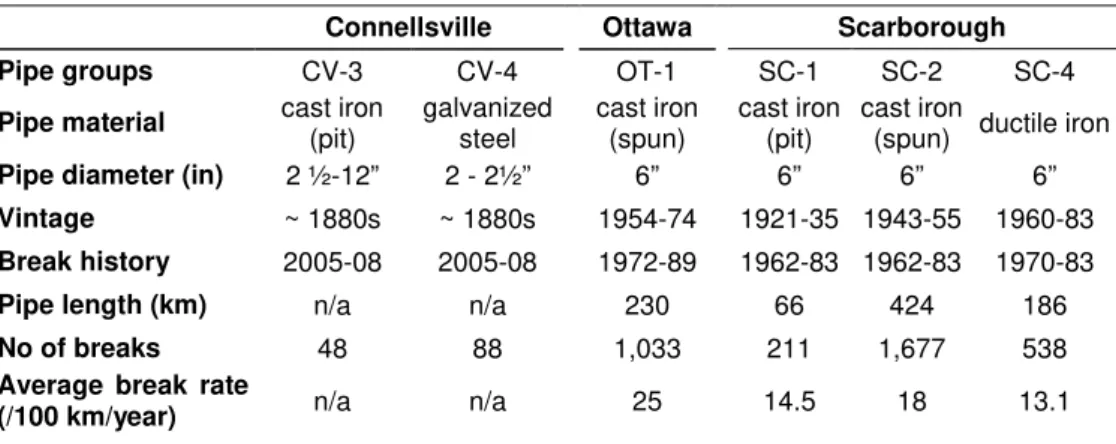
The data sets used for this research comprise six homogeneous pipe groups (with respect to vintage, pipe diameter and pipe material) extracted from data received from three water utilities, Connellsville, Ottawa and Scarborough. (Table 1). In Connellsville, the predominant failure types on galvanized steel pipes were corrosion holes and longitudinal splits, while cast iron pipes had circular breaks, corrosion holes and longitudinal splits. Water temperature was measured once a day, immediately downstream of the treatment plant (which is close to the city). This daily temperature value was assumed in the analysis to represent the mean daily water temperature in the distribution network. The mean daily air temperature was measured at the treatment plant. Groups OT-1 (Ottawa) and SC-1, SC-2 SC4 (Scarborough), comprised pipes that have experienced only circular breaks, longitudinal splits or corrosion holes. Most breaks in SC-4 (ductile iron pipes) were corrosion holes, while in the other groups most breaks were circular (typical of cast iron pipes). Ottawa embarked on a hot spot cathodic protection (HS CP) program in 1990 that likely imposed a substantial change in breakage pattern. Air temperature data for Ottawa and Scarborough were obtained from Environment Canada

Table 1. Data sets used to investigate temperature impact on water main breaks. Connellsville Ottawa Scarborough

Pipe groups CV-3 CV-4 OT-1 SC-1 SC-2 SC-4

Pipe material cast iron (pit) galvanized steel cast iron (spun) cast iron (pit) cast iron

(spun) ductile iron

Pipe diameter (in) 2 ½-12” 2 - 2½” 6” 6” 6” 6”

Vintage ~ 1880s ~ 1880s 1954-74 1921-35 1943-55 1960-83 Break history 2005-08 2005-08 1972-89 1962-83 1962-83 1970-83

Pipe length (km) n/a n/a 230 66 424 186

No of breaks 48 88 1,033 211 1,677 538

Average break rate

(/100 km/year) n/a n/a 25 14.5 18 13.1

The analyses had three objectives: (a) Determine the best time step size, (b) Determine the best threshold values for the degree-day based covariates, and (c) Ascertain which temperature-based covariates are significant.

Time step size. Short time steps capture temperature fluctuations well and provide a large number of data points

but as a consequence also introduce much noise into the sought-after breakage pattern. In contrast long time steps provide smoother breakage rate pattern that tend toward the mean, but result in fewer data points leading to fewer degrees of freedom and poorer model fitting. Further, short time steps (up to 30 days) make the analysis insensitive to the starting point of the analysis period, while longer time steps (90 days or more) require careful selection of a starting point so as not to miss seasonal temperature variations. Also, short time steps {2, 5, 15 days} yield very few breaks per time step, which degrade model fitting (data are small integers and model yields real numbers). Consequently, the selection of time step size requires a balance between the various tradeoffs. Multiple trials were conducted, using the NHP model, to examine in detail how time steps of {5, 15, 30, 60 and 90} days bare on the modeling results. These trials examined each time step, in conjunction with each covariate and with each of the six pipe groups. As expected, these trials showed that �2 values generally improved for longer time steps, however, incremental improvement was inconsistent; (in some trials a large improvement occurred when the time step increased from 60 to 90 days, while in others significant improvement was obtained when the time step increased from the 15 to 30 days. After a careful consideration of all the trials, a time step

(7)

size of 30 days was deemed to be the best choice to balance all the conflicting arguments described above. All subsequent analyses were therefore performed using a 30 day time step.

Air and water threshold temperatures. Several (not exhaustive) trials were conducted with threshold values that

ranged between –10oC and +15oC for air and 0oCto 10oC for water. Trials for groups CV-3 and CV-4 involved simultaneous consideration of air and water temperature-based covariates with different air and water temperature thresholds. Trial for all other groups involved only air temperatures. Examination of the results indicated that the appropriate threshold temperatures are about 0oC to 1oC for air and 4oC for water.

Temperature-based covariates. A three-stage process was used to identify the significant covariates. The first

two stages were to reduce the dimensionality (i.e., number of covariates to be examined) of the problem and the third stage involved an exhaustive enumeration of all combinations of the remaining covariates. In the first stage, cross-correlation was used to identify linear dependence between any pair of covariates. Three covariates, ��_�, ��_� and ��_�, were removed as candidates in the first stage, which resulted in the number of remaining covariates for consideration of 13 for groups CV-3 and CV-4 and 6 for all other groups.In the second stage, trials were only conducted for groups CV-3 and CV-4 in order to further reduce the number (13) of remaining covariates. Using the likelihood ratio (LR) test, it was found that the contributions of covariates ��+ and �� were insignificant (separately and combined) in group CV-4 and were therefore dropped, bringing to 11 the number of covariates to examine for group CV-4. However, these same two covariates made significant contributions in group CV-3, leaving the number of covariates to examine unchanged.

The exhaustive enumeration in the third stage entailed 8192 (13 covariates) trials for group CV-3, 2048 (11 covariates) trials for group CV-4 and 64 (6 covariates) trials for each of the other groups. LR test and ��2 were used to evaluate the trials and it is noted that these two measures did not always agree.

Group CV-3 (cast iron pipe): Seven covariates,��_�+, ��_�−, ��_�+, ��_�, ��_�, ��_�and ��_�, in addition

to the constant αo, emerged as LR-significant. The addition of any other single, pair, triplet or more covariates

was found not to be significant. It is noted that 5 of the 7 significant covariates are based on water temperature and only 2 on air temperature. The application of the ��2measure produced 11 significant covariates (i.e., contributed to incrementally increase the value of ��2), including the 7 LR-significant covariates listed above, and ��_�, ��_�−, ��_�+ and ��_�+. The value of ��2 for the 7 LR-significant covariates was 0.53, and increased to 0.65 for the 11 covariates. Interestingly, the value of ��2 was 0.62 for the entire 13 covariates which is lower (as could be expected) than for the best 11 covariates. The signs of the some of the coefficients of the covariates for CV-3 were found to be contrary to what might intuitively be expected (e.g., a negative coefficient for ��_�, which is expected to be positive).

Group CV-4 (galvanized steel pipe): Three covariates, ��_�−, ��_�, and ��_�, in addition to the constant αo,

emerged as significant. The addition of any other single, pair, triplet or more covariates was found not be significant. Eight covariates were found to be significant based on the ��2measure. These 8 covariates include the 3 LR-significant covariates listed above, and the additional covariates were ��_�, ��_�−, ��_�+, ��_�−and ��_�+. The value of ��2 for the 3 LR-significant covariates was 0.33, and increased to 0.52 with the additional 5 covariates. Interestingly, for the entire 11 covariates the value of ��2was 0.48 (substantially lower than for the best 8 covariates, as could be expected). It is noteworthy that the individual contributions to the LR values of covariates ��_�− and ��_� were small, but their contribution as a pair was very significant. Further, the coefficients of these covariates came out negative indicating that a decrease in their values causes an increase in the number of predicted breaks, which is contrary to what might be expected (elevated intensity of air temperature change, ��_�−, and higher water freezing index, ��_�, are intuitively expected to result in elevated breakage rate). Similarly, coefficients for some of other 8 covariates identified by the ��2 measure were also found to have signs that were contrary to what one would intuitively expect.

Figure 1 illustrates observed and predicted breaks for groups CV-3 and CV-4. It should be noted that the time step size was 30 days and that the “ageing function” was not considered for these groups because ageing is not likely to play a significant role when the analysis period is as short as 3½ years. Figures 3 and 4 show that if both air and water temperatures are available, then the model with LR-significant covariates (7 for CV-3 and 3 for CV-4) is able to predict the observed number of breaks reasonably well. As expected, the comparison is even better with more covariates as obtained by ��2 measure (11 for CV-3 and 8 for CV-4).

The analysis described above for groups CV-3 and CV-4 included both air and water temperature-based covariates. This analysis was repeated using only the 7 air-temperature related covariates. For group CV-3, covariates ��_�+and ��_�, in addition to the constant αo, emerged as LR-significant. An additional

covariate, ��_�, was found significant for CV-4. Using the ��2 measure, the same two covariates were found to be significant for CV-3 and an additional covariate ��_�− was found significant for CV-4. Figure 1 shows that

prediction of water main breaks using only air temperature-based covariates is not as good as when both air and water temperature-based covariates are available.

(8)

Figure 1. Comparison of observed and predicted breaks, groups CV-3 and CV-4

Figure 2. Comparison of observed and predicted breaks, groups OT-1 and SC- 1, SC-2 and SC-4. 0 5 10 15 20 0 50 100 150 200 N o of br e a k s Observed

Predicted - Poisson (w/o ageing, 3 covariates) Predicted - Poisson (w/ageing, 3 covariates)

OT-1 (Cast iron)

R2 = 0.25 R2 _{= 0.36} 0 4 8 0 50 100 150 200 250 N o of br e a k s Observed

SC-1 (Cast iron) SC-1 (Cast iron) R2 _{= 0.22} R2 _{= 0.22} 0 10 20 30 40 0 50 100 150 200 250 N o of br e a k s Observed

SC-2 (Cast iron) R2 _{= 0.64} R2 = 0.74 0 10 20 30 0 50 100 150 N o of br e a k s Time step Observed

Predicted - Poisson (w/o ageing, 1 covariate) Predicted - Poisson (w/ageing, 1 covariate)

SC-4 (Ductile iron₎ R2 _{= 0.028} R2 _{= 0.49} 0 2 4 6 8 0 10 20 30 40 50 N o of br e a k s Time step Observed

Predicted - (11 covariates; air + water) Predicted - LR (7 covariates; air + water) Predicted - LR (2 covariates; air only)

CV-3 (Cast iron) R2 0 2 4 6 8 N o of br e a k s Observed

Predicted - (8 covariates; air + water) Predicted - LR (3 covariates; air + water) Predicted - LR (3 covariates; air only)

CV-4 (Galvanized steel₎

(9)

Group OT-1(cast iron): Three covariates, ��_� , ��_�+, ��_�, were found to be LR-significant. An additional (fourth) covariate, ��_�−, was found significant, using the ��2 measure.

Group SC-1(cast iron): Three covariates,��_�, ��_�−, ��_�+, were found to be LR-significant, of these only the first

two were found significant, using the ��2 measure.

Groups SC-2(cast iron): Three covariates, ��_�, ��_�−, ��_�+, were found to be LR-significant. Four covariates,

��, ��+ , ��− and ��+ were found significant, using the ��2 measure.

Group SC-4 (ductile iron): Only, ��_�, was found significant using both LR and ��2 measures. None of the

covariates was found to be consistently significant in all pipe groups when only air temperature-based covariates were considered. The three covariates found to be the most consistently significant were the average mean air temperature (��_�), maximum air temperature decrease (��_�−), and how fast the air temperature increases over a specific period of days, i.e., ��_�+. Covariates that express maximum air temperature increase (��_�+), and how fast the air temperature decreases over a specific period of days, i.e., ��_�−, were also observed to be significant in 4 of the 6 pipe groups considered in this study. Figure 2 illustrates how the number of predicted and observed breaks compare (with and without the consideration of ageing) for the five groups from Ottawa and Scarborough data (30 day time step). A few observations are noteworthy:

• The NHP model (using different covariates) appears to represent well the number of breaks in group SC-2, but less so in the other groups.

• A significantly higher ��2_{value was obtained for SC-1 when same analysis was conducted using a 60 day} time step instead of 30 days. Group SC-1 is a much smaller group with fewer breaks per time step which is likely to accentuate the issues with predicted real numbers and observed integers for the number of breaks. • The number of breaks in pipe group SC-4 appears to be largely a result of ageing with only minor influence

of temperature-based covariates. This corresponds to the earlier discussion that ductile iron pipes have high ductility and hence do not in general suffer physical fracture but rather fail through the development of perforations by the onset of external corrosion which is time-dependent. This is further corroborated by the significantly higher ageing rate that is apparent in this group.

• Consideration of ageing in group OT-1 increased the goodness of fit measure ��2_{from 0.25 to 0.36. However,} this value is still relatively low compared to values obtained for other pipe groups, likely due to deeper burial depth (2.4 m) of water mains in Ottawa, which would minimize the effects of frost penetration.

5 FINAL COMMENTS

The analyses to assess the impact of temperature-based covariates suggest that water temperature-based covariates can have significant impact on observed breaks as indicated by much higher values of ��2. This influence was most significant in cast iron pipes. However, air temperature-based covariates alone can also explain the main breaks as shown by the high ��2values obtained in the trials for pipe groups OT-1, SC-2, and SC-4. The same covariates are found not to be significant for all pipe groups. As many as 7 to 11 covariates and as few as 1 to 3 covariates were found to be significant, using LR and ��2 measures as goodness of fit, respectively.

Three covariates, namely, average mean air temperature (��_�), maximum air temperature increase and decrease (��_�+ and ��_�−), and how fast the air temperature increase and decrease (intensities) over a specific period of days, i.e., ��_�+ and ��_�−, were found to be the most consistently significant covariates. These covariates concur with some cited observations that the breakage frequency increase when the air temperature transits from above 0oC to below 0oCor vice versa, e.g., during late fall (drop) and early spring (rise).

Signs for some of the coefficients of covariates

were found to be contrary to intuitive

expectation, e.g., decrease in the intensity of air temperature change (��_�−) and decrease in water freezing index (��_�) lead to an increase in predicted breaks. It is possible that some of these covariates work together in a manner that is different from when each covariate is considered on its own.

The availability of both air and water temperature data provided the opportunity to explore their possible influence on water main breaks in three different pipe materials. The analyses showed that different pipe materials can respond differently to temperature-based covariates. The appropriate time step for analysis was identified as 30 days. Few more case studies of the type reported here may be warranted to confirm the influence of water temperature-based covariates on water main breaks.

Acknowledgement

This paper is based on a research project, which was co-sponsored by the Water Research Foundation, the National Research Council of Canada (NRC) and American Water from the United States. Mr. David Hughes

(10)

from American Water led the effort towards the collection of data for Connellsville and his help is duly acknowledged.

References

[1] Walski, T. M. and Pelliccia, A. 1982. “Economic analysis of water main breaks.” Journal American Water

Works Association, 74(3), 140-147.

[2] Newport, R. 1981. “Factors influencing the occurrence of bursts in iron water mains.” Water Supply and

Management, 3, 274-278.

[3] Habibian, A. 1994. “Effect of temperature changes on water-main break.” Journal Transportation

Engineering, ASCE, 120(2), 312-321.

[4] Lochbaum, B. S. 1993. “PSE&G develops models to predict main breaks.” Pipeline and Gas Journal, 20(9), 20-27.

[5] Ahn, J.C., Lee, S.W., Lee, G.S. and Koo, J.Y. 2005. “Predicting water pipe breaks using neural network.”

Water Science and Technology: Water Supply, 5(3-4), 159-172.

[6] Hughes, D., Kleiner, Y., Rajani, B. and Sink, J-E. 2011. “Continuous system acoustic monitoring - from start to repair.” Tailored Collaboration Research Report, Water Research Foundation, Denver, CO.

[7] Goodchild, C.W., Rowson, T.C. and Engelhardt, M.O. 2009. “Making the earth move: Modelling the impact of climate change on water pipeline serviceability.” Computing and Control in the Water Industry 2009:

Integrating Water Systems, University of Sheffield, England. Boxall, J. & Maksimovic, C. (eds). pp.

807-811.

[8] Kleiner, Y. and Rajani, B. 2004. Quantifying effectiveness of cathodic protection in water mains: theory,

Journal of Infrastructure Systems, ASCE, 10(2), 43-51.

[9] Kleiner, Y. and Rajani, B. 2009. “I-WARP: individual water main renewal planner.” Computing and Control

in the Water Industry 2009: Integrating Water Systems, University of Sheffield, England. Boxall, J. &

Maksimovic, C. (eds). pp. 639-644.

[10] Constantine, A. G. and Darroch, J. N. 1993. “Pipeline reliability: stochastic models in engineering technology and management.” S. Osaki, D.N.P. Murthy, eds., World Scientific Publishing Co.

[11] Røstum, J. 2000. “Statistical modelling of pipe failures in water networks”. PhD thesis, Norwegian

University of Science and Technology, Trondheim, Norway.

[12] Kleiner, Y. and Rajani, B. 2003. Forecasting variations and trends in water-main breaks, Journal of