Capacity planning under demand and manufacturing uncertainty for biologics

Capacity Planning under Demand and Manufacturing Uncertainty for Biologics by

Sifo Luo

Master of Science, Information and Service Management, Aalto University, 2015 SUBMITTED TO THE PROGRAM IN SUPPLY CHAIN MANAGEMENT IN PARTIAL FULFILLMENT OF THE REQUIREMENTS FOR THE DEGREE OF

MASTER OF ENGINEERING IN SUPPLY CHAIN MANAGEMENT AT THE

MASSACHUSETTS INSTITUTE OF TECHNOLOGY JUNE 2017

0 2017 Sifo Luo. All rights reserved.

The authors hereby grant to MIT permission to reproduce and to distribute publicly paper and electronic

copies of this thesis document in whole or in part in any medium now known or hereafter created.

Signature of Author...Signature

redacted

tr _{May 12,2017} Certified by... Accepted by...

Sianature redacted

Sir

r

ace

Signature redacted

1'

... Dr. Yossi Sheffi Director, Center for Transportation and Logistics Elisha Gray II Professor of Engineering Systems Professor, Civil and Environmental Engineering

MASSACHUSETTS INSTITUTE OF TECHNOLOGY

AUG 012017

LIBRARIES

Capacity Planning under Demand and Manufacturing Uncertainty for Biologics by

Sifo Luo

Submitted to the Program in Supply Chain Management on May 12, 2017 in Partial Fulfillment of the

Requirements for the Degree of

Master of Engineering in Supply Chain Management

Abstract

Due to the long lead times and complexity in drug development and approval processes, pharmaceutical companies use long range planning to plan their production for the next 10 years. Capacity planning is largely driven by the long-term demand and its forecast uncertainty. The impact of uncertainties at manufacturing level, such as factory productivity and production success rate, are not entirely taken into account since only the average values of each manufacturing parameter are used. Can we better allocate production among manufacturing facilities when both demand and manufacturing uncertainties are considered? In this thesis a stochastic optimization approach is followed to minimize the deviation from target capacity limit under different manufacturing and demand scenarios. The mixed integer linear model incorporates the impact of demand and manufacturing variation on production allocation among manufacturing facilities through Monte Carlo generated scenarios. The thesis model is designed in a way that can be used as a decision tool to perform robust capacity planning at the strategic level.

Thesis Supervisor: Ozgu Turgut

Acknowledgements

I sincerely thank my thesis advisor, Ozgu Turgut, for her valuable guidance and insights that helped me throughout this analysis. I am grateful to Matias and Markus from the sponsor

company for the dedication of their time and resources. This thesis would not have been possible without the guidance and feedback from Bruce Arntzen and Pamela Siska. Additionally, I extend my deep gratitude to my family for their support.

Table of Contents

1

2 LITER A TU R E R EV IEW ... 9

2.1 Pharm aceutical Supply Chain... ₉

2.2 Risks in Biologics Planning ... ₁₀

2.3 M ethodologies ... ₁₁

2.3.1 Supply Chain Risk Assessm ent... ₁₁

2.3.2 M onte Carlo Sim ulation...13

2.3.3 Optim ization...13

2.4 Conclusion...14

3 M ETH O D O L O G Y ... ₁₇

3.1 Overview ... 17

3.2 Data Description ... 18

3.2.1 Dem and Data...18

3.2.2 M anufacturing Param eters ... 19

3.2.3 Site Capacity ... 21

3.3 M odel Description ... 21

3.4 M odel Form ulation...24

4 R E SU LTS & A N A LY SIS... 29

4.1 Capacity Planning under the Default Manufacturing Performance ... 29

4.2 The Im pact of Dem and Variation... 32

4.3 The Im pact of M anufacturing Param eter Variation ... 38

4.3.1 The Effect of Success Rate Variation ... 38

4.3.2 The Effect of Runs per W eek Variation... 40

4.3.3 The Effect of Kilogram s per Run Variation... 42

4.4 M ore Scenarios ... 43

4.4.1 Low SR, Low KGS, and High RW ... 43

4.4.2 High SR, Low KGS, Low RW ... 44

4.4.3 Low SR. High KGS, Low RW ... 46

5 D ISC U SSIO N ... 47

5.1 Dem and V ariation ... 47

5.2 Param eter Variation ... 47

5.3 Baseoloads ... 51

5.4 The Riskiest Scenario...52

5.5 Research Lim itations...54

5.6 Future Studies...55

6 C O N C LU SIO N ... 57

REFER E N C E ... ₅₈

Table of Figures

Figure 1 Biologics supply planning is driven by long-term demand planning... 10

Figure 2 Supply chain risk assessment framework (Deleris & Erhun, 2005)... 12

Figure 3 Simplified biologics supply chain flow and planning process ... 18

Figure 4 Example annual demands under different demand scenarios... 19

Figure 5 Example scenario generation process for success rate (when other two parameters are kept at base values)... 20

Figure 6 Scenario ranges for each manufacturing parameter ... 21

Figure 7 Base loads (utilized capacity) in each facility ... 21

Figure 8 Production allocation under current parameter value and low demand ... 30

Figure 9 Production allocation under current parameter value and base demand ... 30

Figure 10 Production allocation under current parameter value and high demand ... 31

Figure 11 Production allocation comparison between the model result and XYZ Co.'s current p lan ... 32

Figure 12 Production allocation under high success rate and base demand ... 33

Figure 13 Production allocation under high success rate and demand downside... 33

Figure 14 Production allocation under high success rate and demand upside... 34

Figure 15 Raw material production volume under high success rate and demand variation ... 34

Figure 16 Production allocation under high kilograms per run and base demand... 35

Figure 17 Production allocation under high kilograms per run and demand upside ... 35

Figure 18 Production allocation under high kilograms per run and demand downside ... 35

Figure 19 Production volume under high kilograms per run and demand variation ... 36

Figure 20 Production allocation under high runs per week and base demand... 37

Figure 21 Production allocation under high runs per week and demand upside ... 37

Figure 22 Production allocation under high runs per week and demand downside ... 37

Figure 23 Production volume under high runs per week and demand variation ... 38

Figure 24 Production allocation difference between low and high success rate under low demand ... 39

Figure 25 Production allocation difference between low and high success rate under base dem and ... 39

Figure 26 Production allocation difference between low and high success rate demand upside. 39 Figure 27 Extra capacity needed to fulfill the unmet demand under low SR & high demand scenario ... 40

Figure 28 Production allocation difference between low and high runs per week under low dem and ... 4 1 Figure 29 Production allocation difference between low and high runs per week under base dem and ... 4 1 Figure 30 Production allocation difference between low and high runs per week under demand u p sid e ... 4 1 Figure 31 Extra capacity needed to fulfill the unmet demand under low RW & high demand scen ario ... 4 2 Figure 32 Production allocation difference between low and high kgs per run under demand dow n side ... 42 Figure 33 Production allocation difference between low and high kgs per run under base demand ... 4 3

Figure 34 Production allocation difference between low and high kgs per run under demand u p sid e ... 4 3

Figure 35 Unfulfilled demand when demand is upside ... 44

Figure 36 Extra capacity needed when demand is high... 44

Figure 37 Unfulfilled demand when demand is upside ... 45

Figure 38 Extra capacity needed when demand is high... 45

Figure 39 Unfulfilled demand when demand is upside ... 46

Figure 40 Extra capacity needed when demand is high... 46

Figure 41 Capacity deviation comparison between base case scenario and parameter scenarios 48 Figure 42 The low parameters show significance with p value < a (=0.5)... 49

Figure 43 The capacity deviation difference between KGS and RW is not significant ... 50

Figure 44 The capacity deviation difference between RW and SR is not significant ... 50

Figure 45 The capacity deviation difference between KGS and SR is not significant... 51

Figure 46 Production allocation under low manufacturing performance and low demand... 52

Figure 47 No available capacity under low manufacturing performance and high demand ... 53

Figure 48 Unfulfilled demand under low manufacturing performance ... 53

1 INTRODUCTION

Many pharmaceutical companies are turning from conventional small-molecule drugs (like aspirin) to large molecules, biologics derived from living cells (Edwards, 2011). Biologics are used for cancer treatment and other major diseases. These drugs require a much more complex and expensive manufacturing process than small molecules (Ochala, 2015), making biosimilar' competition challenging when patents expire. As a result, biologics play a significant role in company strategy and profitability.

Before drug approval, special industry conditions, such as tough regulatory policies and complicated drug development technologies, add uncertainty to supply chain planning for

biologics. Once the drugs are approved, the challenge is to reliably supply therapies to patients in every market in which the drug has been approved. Constrained supply and time-consuming production setup in compliance require companies to plan far in advance. Therefore,

pharmaceutical companies use range planning as their forecasting timeline. With long-range forecasting, risk and accuracy become important consideration.

Currently, XYZ Co.'s strategic capacity planning is constrained by the long-term demand and its forecast uncertainty. The impact of manufacturing level uncertainties, such as factory

productivity and production success rate, is not entirely taken into account because only the expected self-reported values of production facilities are used. This thesis has two goals. First, it is to evaluate the relative impact of variance of technical parameters on biologics supply

uncertainty. Second, it is to develop a better communication approach around risk and

uncertainty to key company stakeholders. This thesis helps to bridge the gap between long-range demand planning and manufacturing performance in pharmaceutical production planning.

2 LITERATURE REVIEW

This chapter discusses of the risk and uncertainty of pharmaceutical supply planning, followed by an overview of common risk modeling methodologies.

2.1 Pharmaceutical Supply Chain

The main objective of the biologics supply chain is to guarantee supply continuity. Shortage of these products may endanger patients' lives and impact the company's market share. In addition, the lengthy regulatory approval process in this industry prolongs the time it takes to create new manufacturing capacity (Edwards, 2011). Every detail of this process is subject to stringent regulation, including raw materials, plant design, operational processes, etc. Companies tend to invest early in capacity and, on average, a new drug takes 8 to 12 years from patent filing to first

sale (Shah, 2004).

Typically, biologics manufacturing is divided into two parts: the production of the active

pharmaceutical ingredients (API2, also called drug substance) and the production of the finished form in galenical3 units (GU). Supply chain planning begins with demand planning, which usually accounts for 5 to 10 years of sales. Patent expiration and competition account for the

sales life cycle of the biologics. As shown in Figure 1, demand forecasts are based on a

combination of historical data and market intelligence on patient flow, drug dosage, and therapy duration. Supply planning then converts the aggregated market demand data into raw material

2 _{APIs are any substance or mixture of substances intended to be used in the manufacture of a drug product and that, when used}

in the production of a drug, becomes an active ingredient in the drug product (FDA).

API level manufacturing demand. Production planning is driven by long-term demand planning. In many companies, demand planning and supply planning are handled by different functions.

Patients _Dosage Drug Therapy _Duration Demand Planning Market

Demand

Product Demand In Volume

Number of Galenical Units (CapsulesTabletsilals) Manufacturing

Demand

API

(Drug Substance) _{Pfan ng}

Figure 1 Biologics supply planning is driven by long-tern demand planning

2.2 Risks in Biologics Planning

Due to the long-term demand forecast, raw material production is a push process (Shah, 2004). Companies plan production to meet their demand target and give time to prepare a place for stock. Pharmaceutical manufacturers usually hold large stocks of API to avoid stock outs. This means that they are not able to respond quickly to changes in demand, which can result in the bullwhip effect. The bullwhip effect creates turbulence in inventory in response to the demand fluctuation. Companies may consequently end up with excessive safety stock.

In addition to future demand uncertainty, Ochala (2015) describes other typical uncertainties in biologics planning:

* Variation in yields from different manufacturing processes

" Uncertainty in capacity: regulatory or technological specific requirements for certain drugs might affect the production site allocation and migration

* Uncertainty about production site: whether to produce in-house or use contract manufacturers

" External uncertainties: postponed drug approval and sales decline when patents expire

In addition to the risks mentioned above, there are operational factors within a manufacturing facility which affect the amount of output. This thesis will focus on such uncertainties related with in-house production, resulting in productivity or capacity variations.

2.3 Methodologies

Various methodologies have been developed to quantify supply chain risks, with substantial research on probabilistic simulation and programming optimization.

2.3.1 Supply Chain Risk Assessment

Deleris and Erhun (2005) developed a quantitative risk assessment framework to identify key supply chain risk drivers. The overview of this framework is provided in Figure 2.

Analytical Process Information Tools and Output Techniques

Definition of System Expert And Performance Value opinion

Performance measures

Risk Expert

Identification opinionInfluence diagrams

0 _{Risk factors on} staistics,

influence diaram _{Expert Simulation;}

Risk

Risk opinion; probabilistic modeling

Quantification sait

statistics

Probability

distributions Simulation; box plots;

Risk risk curves; decision

Management analysis

Figure 2 Supply chain risk assessment framework (Deleris & Erhun, 2005)

In this framework, Deleris and Erhun start from understanding the critical cost factors in the system. This is continued by risk factor identification. To simplify this process, Deleris and Erhun segregate the supply chain into five distinct components: supply, transportation, production, storage, and demand. Both internal and external risks and their interdependency should be considered in each of these components to give a holistic view of the supply chain risk. These risk factors and the relationships between them are given estimated probabilities. Along with the estimation of the probability of a specific risk scenario, the value of the aggregated risk under the specific scenario can be captured. This framework provides insightful guidance to managerial decisions in risk identification and mitigation. This qualitative framework is applicable in the pharmaceutical industry as the same supply chain components apply within pharmaceuticals. However, due to the uniqueness and complexity in long-range planning in pharmaceutical industry, a different emphasis on risk factors would be required.

2.3.2 Monte Carlo Simulation

Many pharmaceutical companies, including XYZ Co., use Monte Carlo simulation as the main methodology to fuse risk factors into forecasted demand. Monte Carlo simulation is a technique which calculates an output parameter by using repeated random sampling algorithms on input space (Lee, Lv, & Hong, 2013). The result of Monte Carlo simulation provides estimation for different levels of uncertainty. Common practice is dividing the whole uncertainty range into three: downside, upside, and base.

Shah (2004) developed a model to assess the dynamics of the pharmaceutical manufacturing process and business process. Operational uncertainties included product demand, process yields, as well as processing times. In his models, he simulates the effect of different quality control procedures and service levels on finished goods inventory. In this sense, stochastic simulation is a useful tool to quantify expected future performance and its confidence limits.

Lee et al. (2013) applied Monte Carlo simulation to measure the influence of quality inspection levels on manufacturing systems. System performance is studied from the quality and lead time cost perspective. They suggested conducting Monte Carlo simulation in the following steps: (1) Design for what-if analysis; (2) Identify input parameters; (3) Determine the number of trials per run; (4) Conduct output analysis.

2.3.3 Optimization

In risk modeling, optimization models that contain stochastic components of supply, process, and demand are often used; this model can be with single or multiple objectives. Khakdaman et al.

(2015) developed a robust optimization model for production planning. It serves to optimize multiple objectives while considering several types of risk. Under the robust optimization approach, scenarios are taken as inputs; decision variables are divided into design and control variables, of which in the first phase only the control variables are impacted by uncertain

parameters. The model first finds the best values for the control variables and then subsequently optimizes the design variables.

Moghaddam (2015) formulated an algorithm that combines Monte Carlo simulation with goal programming. This hybrid model also uses a multi-objective optimization system to determine the supplier selection and order allocation in the manufacturing process. The main objectives are profit maximization and risk minimization. Monte Carlo is then used to determine the best and worst scenarios of the objectives. Ideal solutions from the goal programming optimization under each scenario are put together and compared.

In many studies, optimization models are used as a method for cost reduction or profit maximization. However, in a pharmaceutical context, cost savings is not typically the top priority, as the margins from drug sales are usually promising. In this thesis, the objective of the optimization model will focus on factory utilization; thus, the capacity related risk is revealed better.

2.4 Conclusion

Demand uncertainty and manufacturing performance uncertainty are the main factors that contribute to the biologics planning risks. Prior research in the pharmaceutical industry dealt

with supply planning and risk assessment separately. This thesis addresses this gap by optimizing capacity utilization in manufacturing factories for biologics drug substances. This is to identify a possible capacity shortage risk while approximating the requirements of a stochastic system better with a robust approach.

XYZ Co. uses Monte Carlo simulation to create scenarios for three different demand levels (upside, base, downside). These different demand scenarios are used as input for the optimization model. Optimization model can be used as a complementary decision tool. It is possible to calculate API (raw material) requirements through Monte Carlo simulation relying on average values of in-house manufacturing parameter. However, it is a problem to connect these numbers to production capacity risk, which can only be observed after site selection and capacity

allocation decisions. Additionally, available data for stochastic components changes based on the manufacturing site being selected. In summary, simulations can be used to conduct a rough analysis on the fluctuations of the total API requirement, assuming the in-house manufacturing parameters are the same across all available production units. This thesis utilizes the provided data better with an approach that takes differences across sites into account. These differences are used to determine the capacity requirements, and hence detect a possible capacity shortage. This thesis uses robust stochastic optimization to close the gap between analysis and outcome by creating an integrated decision tool. Compared with suboptimal heuristic approaches that are used for these purposes, optimization includes many variables and a set of system constraints at the same time. By looking at the system holistically, it increases the reliability of the result. Through optimization model, this thesis provides more precise guidance on manufacturing allocation decisions, and accordingly approximates any overutilization risk more closely. In

addition, by making the optimization model a robust stochastic model, uncertainty in the input parameters are still considered.

3 METHODOLOGY

3.1 Overview

This chapter describes the methodology used to allocate raw material production among different manufacturing sites. Annual drug demand needs to be satisfied while considering each site's capacity target under demand and various manufacturing related uncertainties. The methodology involves narrowing down the drug and site scope, collecting relevant data, developing the capacity utilization optimization model, and testing the results under diverse manufacturing and demand scenarios.

Global pharmaceutical companies must ensure on time delivery of medications to patients around the world. To guarantee this, they plan their manufacturing far ahead to make sure each plant will have enough capacity for any new and existing products. Manufacturing uncertainty together with demand uncertainty create complexity in pharmaceutical supply planning. The right time and location to open or close a production line must be determined. Being able to foresee potential capacity constraint is a key insight from the manufacturing planning point of view. Figure 3 shows a simplified supply chain flow of biologics from API manufacturing to being delivered to the patients, but the production planning started from a reverse direction. It starts from patient demand, and the demand is converted to smaller units of drugs, the raw materials, to the number of production runs, and finally to the estimated production time. This thesis will focus on the drug substance manufacturing portion of the process. Here, a model is developed to provide decision support for allocating production among different manufacturing sites under various demand and manufacturing capability scenarios. The goal is to achieve robust

plant capacity utilization under different uncertainty scenarios.

How biologics are planned from demand to manufacturing

Plan*n, g P ow Simp'ed biofogcs sappip ctain

"t Det"'" Market emanFinp]

in Galenical Units In Cslenical Unfts

In kas D"u ProduOt

t WeekS Produsu

Conversion Factor success Filing throughput Packaging throughput rate * kgs per run * run per

week

Figure 3 Simplified biologics supply chain flow and planning process

3.2 Data Description

Data collection was conducted through company site visit, company calls and interviews with the company's long range planning team.

3.2.1 Demand Data

This study uses the data of a single drug and the three manufacturing factories where it is

produced. The annual demand data consists of global demand projections for this drug from year 2018 to year 2025. An estimation of galenical units needed for drug X was converted to drug substance demand in kilograms. Currently, XYZ Co. allocates drug substance demand to each manufacturing facility through a combination of regional demand estimation and regulatory

constraints. Demand forecast data in the model is used as given, as the values derived from the current process are not being evaluated in this methodology.

To account for the variation in demand, three scenarios were generated: base case, upside case, and downside case. These scenarios were generated from the Monte Carlo simulation

methodology discussed in the literature review. Figure 4 shows a sample data of yearly aggregated demand under three different scenarios. The combined annual throughput of manufacturing sites needs to fulfill the yearly demand in all scenarios.

Demand Basecase Drug X API IfRegion 1 140.01 155.28 163.06 130.89 111. 94 113. 46 99. 47 126.88

Demand Basecase Drug X AP I Region 2 223. 16 246.79 280.86 288. 28 270.50 279.50 248.10 343.75

Demand Basecase Drug X API 1 Region 3 267.64 267.23 193.66 149.28 128.63 130.82 116.34 143.38

Bse Scenario Annual Oemand 630.79 669.30 627.57 561.44 511.08 523.78 462.92 614.01

Demand Downside Drug X API 1 Region 1 93.34 137.01 107.14 80.13 67.17 61.89 59.68 29.28

Demand Downside Drug X API 1 Region 2 193.56 203.45 214.80 198.58 175.97 179.48 157.09 216. 49

Demand Downside Drug X API 1 Region 3 230.84 212.36 145.93 107.39 87.94 86.80 75.52 93.16

Downside Scenario Annual Demand 517.74 552.81 467.87 386.20 331.06 328.17 292.29 333.92 Demand Lpside Drug X API I Region 1 185.01 175.00 166.79 178.77 151.18 133.75 103.26 160.96

Demand Upside Drug X API 1 Region 2 251.20 295.22 366.16 414.43 422.68 446.27 396.07 550.08

Demand Upside Drug X API 1 Region 3 309.11 337.05 278.51 255.72 256.17 279.13 245. 15 303.91

Upside Scenario Annual Demand 745.32 3W7.27 811.45 148.92 130.03 859.15 744.47 1,014.95

Figure 4 Example annual demands under different demand scenarios

3.2.2 Manufacturing Parameters

Three technical parameters related with API manufacturing were chosen by XYZ Co. in this study

- success rate, runs per week, and kilograms per run. Success rate is the expected ratio of runs (batches) that are successfully made (where product meets all regulatory specifications) over total batches. Runs per week and kilograms per run represent the output capability of each facility. Runs per week measures how many batches the site can run, given how long it takes to do a run based on all equipment that is being used. Kilograms per run is the average amount of material expected from a batch. Currently in XYZ Co., these parameters are defaulted to be constant numbers across

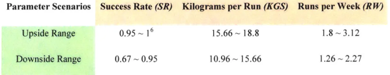
all facilities, based on either regulation expectation or testing results. In production, these parameters should be measured based on the advancement of manufacturing technology. To measure the influence of floating manufacturing parameters, two scenarios -- upside and downside -- were created for each parameter assuming all of them were uniformly distributed between observed maximum and minimum value over the years4_{. The maximum upside value is 10% high}

than the base value, and the minimum downside value is 30% lower than the base value5_.

Combining three demand scenarios, there are in total 18 (= 6 manufacturing parameter scenarios

* 3 demand scenarios) scenarios. Schema for scenario generation is depicted in the Figure 5 for one of the stochastic parameters -- success rate -- under study. Figure 6 shows the ranges used in different manufacturing performance scenarios. Equal manufacturing rates are used across all demand levels in order to observe the effect of demand variation. The effect of demand variability is revealed through using randomly generated technical parameter scenarios at various demand levels, while the effect of variability in technical parameters is shown by constructing different input sets.

Manufaacrumiq unLt U rtam lws Demand Uncertainties

Successsweario 1.Demand

Su ess _Downside

Kgs per Run Wu n se Downsideper

Base Case Case SceDowns

Success ceario 5 Demand

Rate Upside Basecase

Demand

Upside

Figure 5 Example scenario generation process for success rate (when other two parameters are kept at base values)

4 The upside and downside scenarios of the three manufacturing parameters are generated based on base values provided by XYZ

Co.

Parameter Scenarios Success Rate (SR) Kilograms per Run (KGS) Runs per Week (RJ*)

Upside Range 0.95 ~ 16 15.66'-18.8 1.8--~3.12

Downside Range 0.67 0.95 10.96 - 15.66 1.26 -2.27

Figure 6 Scenario ranges for each nanufacturing paraneter

3.2.3 Site Capacity

Capacity of manufacturing facilities is measured in weeks. The full capacity of each site is 52 weeks, and each site is identical with respect to the target capacity (80% of full capacity) and minimum target capacity (50% of full capacity). Each manufacturing site runs many production lines (i.e. produce multiple drug substances). The utilized capacity of a site for other drugs is captured as a baseload. Figure 7 shows the capacity taken by existing production lines in each factory. The combined throughput of all manufacturing sites needs to satisfy the annual demand while keeping the capacity utilization optimal.

Takb Cspmdlylu Einh Pracdim Sib (mmrdla wein .)

Year 2018 Year 2019 Year 2020 Year 2021 Year 2022 Year 2023 Year 2024 Year 2025 Site A 13.0 4.6 12.2 13.5 14.2 12.5 18.6 8.4

Site B 18.5 11.7 17.5 22.4 18.9 21.2 22.2 28.6

Site C 23.7 26.8 28.8 26.8 21.2 29.7 30.6 31.1

Figure 7 Base loads (utilized capacity) in each facility

3.3 Model Description

The thesis is narrowed in scope one biologic and its three manufacturing sites. The active ingredient API of medicine X is manufactured in different factories M in year T. The site capacity is measured in weeks W of production. The utilized capacity of a site for other

production lines is captured as Base Usage. This model assumes that Base Usage representing the

6 Unlike the other two parameters, parameter SR's upside scale is less than 10%. This is because the given SR base value is very

existing production lines in each facility is pre-determined and cannot be re-allocated. The main decision variable of the model is denoted as ThputM, which represents the amount that should be produced by each site. In the model, the total of ThputM that is allocated to each site should be equal to the yearly demand forecast. Demand is measured in kilograms. Thus, on the other side of the equation, ThputM is measured in kilograms as well. In addition, capacity is measured in weeks at the strategic level. For that reason, ThputM is converted to Weeks by dividing this quantity to three manufacturing parameters: Success Rate SR, Kgs per Run KGS, and Run per Week R W. To measure the effect of manufacturing performance variation on capacity planning, various scenarios were created by generating random values for these three parameters from the upside to the downside ranges. Similarly, to factor the demand uncertainty into capacity

planning, these scenarios were supplemented with random values of drug substance demand D. Demand scenario set DL consists of upside, base, and downside values of demand.

Scenarios of a single run are formed as follows: the particular model under focus is used to assess the effect of success rate (SR) on capacity allocation. Within the lower percentile of the SR range and the low demand range, n scenarios for success rate were created as the result of both Monte Carlo simulation. This scenario creation process was repeated for all demand levels, while maintaining the generation of random SR values from the same range. Therefore, in total, 3*n scenarios were obtained per a single optimization run. Meanwhile, all but one stochastic

manufacturing parameter were kept the same at their base value across the set. After getting the results of this optimization run, the same input preparation procedure was repeated this time using a high range of the same parameter. Finally, optimization results over this second set were compared with the first set in order to identify the effect of the SR parameter on capacity

planning and allocation. Different sets of inputs are built in order to observe the effects of each stochastic component on the manufacturing capacity risk. The first set of experiments is performed by varying a single factor in the inputs at a time. Then, combinations of different factors are chosen in order to observe the blended effects.

As this drug is vital for cancer patients, the throughput of manufacturing ThputM must be at least at a level that will fulfill the aggregated drug substance demand. The total utilization of each site is set to be between the minimum target capacity and the full capacity. As mentioned earlier, the base time unit in the model is a year. It is assumed that each year's demand is independent of other years. In other words, there is no stocking decision made in the model. This model assumes that production of medicine X can be freely moved between sites for optimal capacity utilization. Hence, the model tries to distribute the week-based capacity utilization among allocated sites evenly. However, a new site which has zero baseload will only be allocated when the existing sites' maximum capacity is reached. In addition, this model captures the unsatisfied demand as SlackThput and excess amount of production above the demand as ExtraThput. ExtraThput

compensates for overproduction, while SlackThput represents the amount of underproduction.

The model used in this study is a robust optimization model. That is, it takes into account several probabilistic scenarios and makes the decision based on the worst case. Although the model applies an even allocation policy among available sites, the ones with the maximum capacity requirements are emphasized in the outputs. This is done in order to detect capacity shortage cases with greater confidence. There is no cost related objective in this model, as it is purely capacity based. The mathematical formulation of the model is presented below.

3.4 Model Formulation

set of manufacturing factories/sites timeframe in years {2018...2025} active pharmaceutical ingredient

set of demand levels

{

Parameters: SR RW KGS D BaseUsage

manufacturing success rate per site (stochastic per M, T, API, DL, S) number of production runs per week (stochastic per M, T, API, DL, S) kilograms of API per production run (stochastic per M, T, API, DL, S) drug substance requirement, in kilograms (stochastic per T, API, DL, S) utilized capacity of each site, in weeks

Decision Variables:

ThputM Non-negative variable to capture manufacturing amount, in kilograms (per M, T, API, DL, S)

SlackThput Non-negative variable to capture manufacturing volume in case extra capacity is needed, in kilograms (per T, API, DL, S)

ExtraThput Non-negative variable to capture manufacturing volume in case total capacity does not reach the minimum capacity level, in kilograms (per T, API, DL, S)

W Non-negative variable to capture site capacity utilization measured in weeks (per M, T, API, DL, S) Sets: M T API DL S

P Binary variable showing whether or not a site is used (per M, T, API, DL, S) (1 =the site is used for production, O=the site is not used for production)

FinalWeeks Non-negative variable showing the maximum of Weeks among all scenarios of a demand level set (per M, T, API, DL)

XW+ Non-negative variable captures the excess of 'Weeks+BaseUsage' from target value (i.e. 80% of 52 weeks) (per M, T, API, DL, S)

XW~ Non-negative variable captures the slack of 'Weeks+BaseUsage' from target value (i.e. 80% of 52 weeks) (per M, T, API, DL, S)

Part 1:

Objective function:

Min || W + BaseUsage - Target Capacity ||

Subject to:

(Week capacity conversion constraint)

W (m, t, s, api, dl) = ThputM(m,t,s,dI,api) Vm E M, t E T, a E API, dl E SR(m,t,s,dl,api) * RW(m,t,s,dl,api) * KGS(m,t,s,dl,api)

DL,s - S

(Throughput-Demand relation constraint)

ThputM = D

(Week capacity bounds)

Minimum Target Capacity - BaseUsage W 5 Site Full Capacity - BaseUsage

(Robust capacity requirement definition)

Where full capacity is 100% (52 weeks), target capacity is 80% * 52 weeks, which is 41.6 weeks, and Minimum Target Capacity is 50% * 52 weeks, which is 26 weeks. The above

formulation contains several non-linear mathematical expressions. The first of these terms is max W. This is the result of the robust optimization strategy mentioned above (in order to represent the maximum of W variable). The second of the nonlinear component is the absolute value in the objective function. This expresses the deviation, the positive or negative difference, from the target capacity. In order to solve this model with a linear solver, the following linear

programming formulation (Part 2) is implemented by adding three new decision variables, namely FinalWeeks, XW+ and XW-.

Part 2:

Objective function:

Min EM,T,API,DL,S(XW +m,t,api,dl,s + XW-m,tapi,d1,s + U1 * P m,t,api,dl,s) +

U2 * ZT,API,DL,S(ExtraThput t,api,dl,s + SlackThput t,api,dl,s) ₍₁₎

Where U1 is a small penalty number that limits the total allocated number of sites for production;

U2 is a big penalty number for using extra capacity when the existing capacity is not maxed out

or underutilizing a facility that creates non-negative slack capacity.

Subject to:

(Week capacity conversion constraint)

W = _{SR(m,t,s,api,dl)} ThputM(m,t,s,api,dl) _* Vm E M, t E T, api E API, dl E DL, s E S (2)

RW(m,t,s,api,dl) * KGS(m,t,s,api,dl)

Em ThputM m,t,api,d1 ExtraThput t,api,d1,s + SlackThput t,api,dl,s = Dm, t, api, dl,s

(Week capacity bounds)

Minimum Target Capacity * Pm,t,api,d ,s < Wm,t,api,d1,s + BaseUsage

Wm,t,api,dl,s + BaseUsage Site Full Capacity * Pm,t,api,dl,s

(where P is functional when BaseUsage =0; i.e. if W = 0 & BaseUsage = 0, P =0)

(FinalWeeks definition constraint)

FinalWeeks m,t,api,dl -> Wm,t,api,dI,s Vm E M, t E T, api E API, dl E L

(Definition constraint for positive deviation from target capacity)

Wmt,api,dl,s - Target Capacity XW-m,t,api,dl Vm G M, t C T, api e API, dl

(Definition constraint for negative deviation from target capacity)

Target Capacity - Wm,t,api,dL,s XW~m,t,api,d1 Vm E M, t E T, api E API, dl

(3) (4) (5) L,s E S E DL E DL

(1) The objective function has three parts. Part one is about capacity allocation through minimizing the deviation from the target capacity limit; part two is about site selection by minimizing the site used; part three is about demand fulfillment through minimizing the unsatisfied or excess demand respectively.

(2) Capacity conversion constraint describes the way XYZ Co. measures capacity of their manufacturing facilities. Capacity is measured in weeks through dividing the yearly production volume by the conversion factor -- runs per week multiplies kilograms per run multiplies success rate.

(3) Demand constraint limits the annual production volume to be as close to the annual demand as possible. If total ThputM-- production in kilograms -- exceeds demand, ExtraThput is positive; if it is under demand, SlackThput is positive. SlackThput and ExtraThput are

(6)

(7)

auxiliary decision variables that are used to prevent infeasibility of the model in case demand cannot match exactly with the production volume.

(4) Upper capacity limit constraint: Site binary variable P is determined by capacity Wand taken capacity Base Usage. Only when Wand Base Usage are 0, P is 0.

(5) Lower capacity bound: to make sure P is 1 if the sum of Wm,t,apii,d s and Base Usage is positive.

(6) Among all the scenario solutions, FinalWeeks takes the riskiest capacity usage among scenarios of each demand level set. This is to guarantee the robustness of the approximation for a capacity utilization risk i.e. overutilization.

(7) This defines the positive deviation from target capacity: W+BaseUsage > Target (8) This defines the negative deviation from target capacity: Target > W+BaseUsage

The model aims to minimize the distance between the target capacity and each site's total capacity utilization, including drug X and other production lines. This model is robust in the sense that only the scenario which requires most capacity is shown in the representations. This is to approximate an over- or under-utilization risk of manufacturing capacity with greater

4 RESULTS & ANALYSIS

This section presents the production allocation results from the optimization model. The model is built using Julia's optimization language JuMP. The model has 536 constraints and 480 variables after presolve. The variation of allocation among manufacturing facilities under different demand and technology scenarios is discussed.

The model tries to limit the production to as few facilities as possible while fulfilling the annual demand requirement. This means that site that has the smallest deviation from the target capacity level will be allocated first. As a result, the model prioritizes production at sites that reach the capacity more easily. At the same time, the model also avoids the under-utilization of a facility. The results below demonstrate the influence of different manufacturing and demand

circumstances on production allocation.

4.1 Capacity Planning under the Default Manufacturing Performance

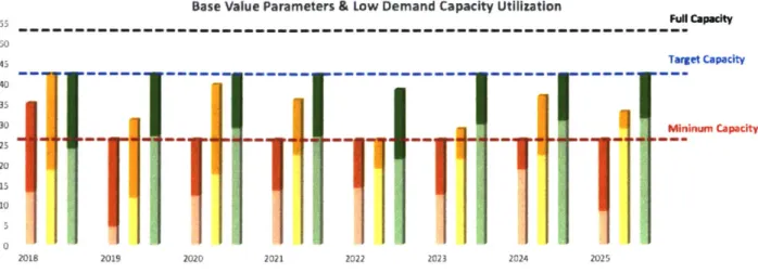
Currently XYZ Co. uses all three manufacturing parameters in their base (default) values in production planning. Across all demand levels (Figure 8, 9, 10), the base case scenario shows there is no risk of running out of production capacity within current facilities in the next eight years. However, when demand peaks, the majority of sites are running above the target capacity.

Base Value Parameters & Low Demand Capacity Utilization Ful Capacity 50 45 Target Capacity 40 35 30 Mininum Capacity 25 20 15

3

I

1 Site A Base U Site A Site B Base U Site B ' Site C Base N Site C

Figure 8 Production allocation under current parameter value and low demand

Base Value Parameters & Base Demand Capacity Utilization

55 ... 50 45 Target Capadty 40 35 30 Minimum Capadty 25 20 15 5 a 2018 2019 2020 2021 2022 2023 2024 2025 Site A Base U Site A Site B Base 4 Site 8 0 Site C Base N Site C

Base Value Parameters & High Demand Capacity Utilization FSgr rl Capat 50 4d Target Capacty 40 35 30 MinseBm Capaadt 25 20 10 Z018 2019 2020 2021 2022 20231 2024 2025

Site A Base U Site A Site B Base 6 Site B o Site C Base U Site C

Figure 10 Production allocation under current parameter value and high demand

Compared with drug X's current allocation plan in XYZ Co. given at the top of Figure 11, the

model optimizes the deviation from the target capacity level. When optimized, as shown at the

bottom of Figure 11, both the deviation and variation in demand satisfied by each facility is

reduced to a more constant level. This consistency is more evident in the optimized model results

XYZ g' Current Production Allocation for Drug X under Default Parameters & Base Demand 5. 50 45 arge:tu 40 35 30 _iiu 25

102:

f

Site A Base a Site A Site B Base 'Site B Site C Base a Site C Production Allocation Decision from the Model under Default Parameters L Base Demand

55- -.--.-..-.-.-- ...- -- .-.-.- ... -.. ..1411 so 45 Target 40 35 301 25 20 1.5 nimu 013 2019 22 . 2D27 2 1 2024 232s

Site A Base * Site A Site 8 Base USiteB Site C Base E Site C

Figure I I Production allocation comparison between the model result and XYZ Co. 's current plan

4.2 The Impact of Demand Variation

Under the same (high) success rate (SR) scenario, where runs per week and kgs per run are kept at base value, capacity utilization is affected by various demand scenarios. At the base demand level (Figure 12), two of three production sites approach or meet the target capacity for the next eight years. As Site C has the highest baseload and hence the shortest distance to the target capacity level, Site C has a higher priority in allocation. Similarly, Site A has the lowest baseload and hence the longest distance to the target capacity level, so it has the lowest priority in

allocation. Therefore, many years Site A misses the target capacity. As a result, Site A in most years needs to produce more than Site C to reach the minimum capacity requirement.

High SR Base Demand Capacity Utilization 55 Full Capacity 50 45 Target Capacity 40 35 30 W~*--MnimumnCapdt

20

--I

Site A Base * Site A Site B Base 0 Site B Site C Base a Site C

Figure 12 Production allocation under high success rate and base demand

Under the downside demand scenario (Figure 13), all sites are producing less and lower site utilization is required. If Site A does not have existing baseloads, it may not be utilized because the model would first fully utilize the other manufacturing facilities.

High SR Low Demand Capacity Utilization

55 Full Capacty so 45 Target Capacity 40 35 30 MnmmCpf 25 ~ ~

"E

Figure 13 Production allocation under high success rate and demand downside

Under the upside demand scenario (Figure 14), the site usage and production volume increase accordingly. Since Site A has the lowest priority in allocation, it ends up producing more to meet the remaining demand. Figure 15 shows the production volumes of three sites under different

demand scenarios. As demand increases, production volume increases. Site C produces the least because it has the highest baseload and the smallest distance to the target capacity level.

High SR High Demand Capacity Utilization

55 FuN Caacity 5 45 Target Capacity 40 35 30 PBinm Ceadty 25 20 15 10 5 e -2018 2019 2020 2021 2022 2023 2024 2025

Site A Base 0 Site A Site 6 Base * Site B S;,e C Base 0 Site C

Figure 14 Production allocation under high success rate and demand upside

Site A Production Volume Site B Production Volume Site C Production Volume K ograns Kograms Kilograms

UDO [200

1000

E*3001

Iwo2 2GOO 600

21 29 22 22 22 22 24 222015 201 2020 2021 222 2023 2024 2020 2218 201 2020 2021 2022 2023 224 2025 Demand Downside 0 Demand Base a Demand Upside Demand Downside a Demand Base U Demand Upside Demand Downside N Demand Base a Demand Upside

Figure 15 Raw material production volume under high success rate and demand variation

Under the same (high) kilograms per run (KGS) scenario (Figure 16, 17, 18), where runs per week and success rate are kept at base value, manufacturing sites are more occupied when demand is higher. Most of the sites can reach the target capacity under upside demand. When demand is lower, some sites produce just enough to reach the minimum capacity level. In demand downside scenario, Site A and Site C can fit in more production lines.

High KGS Base Demand Capacity Utilization 55 Full Capacity 50 45 Target Capacity 40 35 30 MWnlmn Capadty

251I

I

Site A Base U Site A Site B Base E Site B -Site C Base U Site C

Figure 16 Production allocation under high kilograms per run and base demand

High KGS High Demand Capacity Utilization

55 Capacity 50 45 Targe Capacity 40 35 30 Pvlnlmum Capcit 25J 20 15 10 2018 2019 2020 2021 2022 2023 2024 2025

Site A Base 0 Site A Site B Base 0 Site 8 d Site C Base U Site C

Figure 17 Production allocation under high kilograms per run and demand upside

High KGS Low Demand Capacity Utilization

55 Full Capacity 50 45 Target Capacity 40 35 30 Minlnum Capacity 20 2018 2019 2020 2021 2022 2023 2024 2025

Site A Base I Site A Site B Base S Site B * Site C Base N Site C

Figure 19 depicts the production volumes of three sites under different demand scenarios. Site C produces the least because it has the highest baseload and the smallest distance to the target capacity level.

Site A Production Volume Site B Production Volume Site C Production Volume

4gre 9ogream e nd d a 14010 1220 10m 120 4J 0200 28 2 01 2020 20ZI2U2 22 4 22 2018 2019 2020 2021 2022 2023 2024 22022022502 03 204 22

Demand Downside U Demand Base U Demand Upside Demand Downside a Demaed Base U Demand Upside Demand Downside U Demand Base U Demand Upside

Figure 19 Production volume under high kilograms per run and demzand variation

Under the same (high) runs per week (RW) scenario (Figure 20, 21, 22), where kgs per run and success rate are kept at base value, Site B and C are optimally utilized most of the time when demand is at base and upside levels. When demand peaks, as seen in the upside demand

scenario, Site A increases utilization and produces significantly more. When demand decreases, as seen in the downside demand scenario, Site A maintains at the lowest capacity level. When demand is lower than the base level, Site B reduces production significantly and stops production in year 2025. Figure 23 shows the production volume changes across different demand scenarios.

High RW Base Demand Capacity Utilization 55 Full Capacity 55 50 45Target Capacity 45 40 35 30

jMinkmwn

111

jq

Site A Base N Site A Site B Base N Site B 1' Site C Base U Site C

Figure 20 Production allocation under high runs per week and base demand

High RW High Demand Capacity Utilization

55 Ful Capact 50 45 Taruet Capacty 40 35 30 fvlnWMia Capacit 25f 20

f

f

Site A Base R Site A Site B Base 8 Site B e Site C Base U Site C

Figure 21 Production allocation under high runs per i'eek and demand upside

High RW Low Demand Capacity Utilization

55 FAI Capacity 50 45 -- Target Capacity 40 35 30 Mininum Capacity 25 20 10 5 2018 2019 2020 2021 2022 2023 2024 2025

Site A Production Volume Site B Production Volume kilograms Kilogra-Ps 1530 1500 1000 IO 500 500 2019 2O9 2020 2021 2022 2023 2024 2025 2018 2019 2020 2021 2022 2023 2024 2025

Demand Downside 0 Demand Base a Demand Upside Demand Downside a Demand Base U Demand Upside

Figure 23 Production volume under high runs per week and demand variation

Site C Production Volume Kdograms 1000 6o0 430 200 0 2018 2019 2020 2021 2022 202 2024 2025

Demand Downside U Demand Base U Demand Upside

4.3 The Impact of Manufacturing Parameter Variation

4.3.1 The Effect of Success Rate Variation

Compared with the high success rate scenarios , low success rate scenarios utilize sites at higher

capacity. Although the manufacturing success rate is changed, the combined annual production volume of the three sites should be equal to the production volume under the same demand

scenarios. However, as Figure 24, 25, and 26 show, with lower success rate, sites are running more weeks to produce the same volume. Especially when demand is higher, many sites run at

full capacities under low success rate scenario. Low success rate, caused by poor equipment performance or malfunction, boosts up the manufacturing facility capacity utilization across

sites. In high demand scenario, low success rate creates unfulfilled demand in year 2023 and year 2024. Figure 27 shows the extra capacity needed to satisfy the annual forecasted demand.

In high success rate scenarios, SR values are kept at upside level, and the other two parameters are kept at base values. 8 _{In low success rate scenarios, SR values are kept at downside level, and the other two parameters are kept at base values.}

High SR Low Demand Capacity Utilization Low SR Low Demand Capacity Utilization 55--- mm--- Full 50 45--- --- --- - - - -.Target 35 30 _ iiu 25

3

Site ABase NESite A Site 8 Base 4 Site B itSite C Base ESite C

Figure 24 Production allocation difference between low and high success rate under lou, demand

High SR Base Demand Capacity Utilization Low SR Base Demand Capacity Utilization

45 - - - - - - Target .

30 Minimum

Ui25--

-"-.--~-P-2018 2019 2020 2021 2022 2023 2024 2025 2018 2019 2020 202' 2022 2023 2024 2025

Site A Base 5 Site A Site B Base 6 Site 8 10 Site C Base 0 Site C

Figure 25 Producion allocation difference between low and high success rate under base demand

High SR High Demand Capacity Utilization Low SR High Demand Capacity Utilization

so -' -Full 45 40 -

fTarget

1

"Site ABase E Site A SiteB8Base U Site B 6 Site C Base E Site C

Extra Capacity Needed under Low SR & High Demand Weeks 55Full Capacit 50 45 Target Capadty 40 35 30 Minimum Capacity 25 20 is 10 19 55.12 0 2018 2019 2020 2021 2022 2023 2024 2025 U Extra Capacity Needed

Figure 27 Extra capacity needed tofu/fill the unmet demand under low SR & high demand scenario

4.3.2 The Effect of Runs per Week Variation

Runs per week (RW) is the maximum number of batches of a certain product that the site can run per week. If a facility has fewer production runs per week, it demonstrates reduced

manufacturing capability. Under a lower RW9, manufacturing sites need to spend more time to produce the same volume. As Figure 28, 29, and 30 show, compared with high runs per week

scenarios, low runs per week increase the production site utilization significantly. Especially when demand rises, as seen in the demand upside scenario, all sites approach their full capacity level. This puts year 2023 and year 2024 out of capacity to fulfill the forecasted demand. Figure 31 shows the extra capacity in need. When demand shrinks, as seen in the demand downside scenario, Site B is more optimally utilized at a lower RW.

9 In high RW scenarios, RW values are kept at upside level, and the other two parameters are kept at base values. In low RW scenarios, RW values are kept at downside level, and the other two parameters are kept at base values.

High RW Low Demand Capacity Utilization Low RW Low Demand Capacity Utilization 55 ---..-.--- F-i so 45, . ..----.-- -.---. - - -- - - ... -.-. - Target 40 35 30- I -M Minimum 25D-15

I

Site A Base E Site A Site B Base 6 SiteB Site C Base E Site C Figure 28 Production allocation difference between low and high runs per week under low demand

High RW Base Demand Capacity Utilization Low RW Base Demand Capacity Utilization

55 --- ---...-.-.-.-..--.---. --- --- --- --- Full so 45 Tre 40 -35-I

i

I-

20IF1a

t

Site A Base I Site A Site B Base N Site B X Site C Base 1 Site C

Figure 29 Production allocation difference between low and high runs per week under base demand

High RW High Demand Capacity Utilization Low RW High Demand Capacity Utilization

55~~~~~~~~~~~ ~ ~ ~ ~ ~ ~ - -- --- - Full 5o 45 - - - -- - - Target 40 35 - - - - -Minimum 25 20 15 2018 2019 2020 2021 2022 2023 2024 2025 2018 2019 2020 2021 2022 2023 2024 2025

* Site A Base U Site A Site B Base 8 Site B * Site C Base U Site C

Weeks Extra Capacity Needed under Low RW & High Demand 55 Full capacity 50 45 Target Capacity 40 35 30 Mnimum Capacity 25 20 10 ₂ 6.1 5 29 0 U[ 2018 2019 2020 2021 2022 223 2024 2025

0 Extra Capacity Needed

Figure 31 Extra capacity needed tofu/fill the unmet demand under low RW & high demand scenario

4.3.3 The Effect of Kilograms per Run Variation

When the manufacturing process or technology carries lower kilograms per run (KGS), the facility needs more runs to produce the same volume. As Figure 32, 33, and 34 show, under lower KGS scenariol0, all sites are more utilized. When demand is lower, there are extra capacities among three sites to fit in other production lines. However, when demand is at the upside level, all three sites approach full capacity. The annual demand requirements are met in all scenarios.

High KGS Low Demand Capacity Utilization Low KGS Low Demand Capacity Utilization

--- _Ful so 1 -Target

30

11

I

f

I Site A Base E Site A Site B Base E Site B * Site C Base E Site C

Figure 32 Production allocation difference between low and high kgs per run under demand downside

10 In high KGS scenarios, KGS values are kept at upside level, and the other two parameters are kept at base values. In low KGS scenarios, KGS values are kept at downside level, and the other two parameters are kept at base values.