Mind the rate ! Why rate of global climate change matters, and how much

HAL Id: hal-00866404

https://hal.archives-ouvertes.fr/hal-00866404

Preprint submitted on 30 Sep 2013

HAL is a multi-disciplinary open access

archive for the deposit and dissemination of sci-entific research documents, whether they are pub-lished or not. The documents may come from teaching and research institutions in France or abroad, or from public or private research centers.

L’archive ouverte pluridisciplinaire HAL, est destinée au dépôt et à la diffusion de documents scientifiques de niveau recherche, publiés ou non, émanant des établissements d’enseignement et de recherche français ou étrangers, des laboratoires publics ou privés.

Mind the rate ! Why rate of global climate change

matters, and how much

Philippe Ambrosi

To cite this version:

Philippe Ambrosi. Mind the rate ! Why rate of global climate change matters, and how much. 2005. �hal-00866404�

DOCUMENTS DE TRAVAIL / WORKING PAPERS

No 04-2006

Mind the rate!

Why rate of global climate change matters, and

how much.

Philippe Ambrosi

SEPTEMBRE 2005

C.I.R.E.D.

Centre International de Recherches sur l'Environnement et le Développement UMR8568CNRS/EHESS/ENPC/ENGREF

UMR CIRAD

45 bis, avenue de la Belle Gabrielle F-94736 Nogent sur Marne CEDEX

Abstract

To assess climate policies in a cost-efficiency framework with constraints on the magnitude and rate of global climate change, we have built RESPONSE_ , an optimal control integrated assessment model. Our results show that the uncertainty about climate sensitivity leads to significant short-term mitigation efforts all the more as the arrival of information regarding this parameter is belated. There exists thus a high opportunity cost to know before 2030 the true value of this parameter, which is not totally granted so far. Given this uncertainty, a +2 °C objective could lead to rather stringent policy recommendations for the coming decades and might prove unacceptable. Furthermore, the uncertainty about climate sensitivity magnifies the influence of the rate constraint on short-term decision, leading to rather stringent policy recommendations for the coming decades. This result is particularly robust to the choice of discount rate and to the beliefs of the decision-maker about climate sensitivity. We finally show that the uncertainty about the rate constraint is even more important for short-term decision than the uncertainty about climate sensitivity or magnitude of warming. This means that the critical rate of climate change, i.e. a transient characteristic of climate risks, matters much more than the long-term objective of climate policy, i.e. the critical magnitude of climate change. Therefore, research should be aimed at better characterising climate change risks in view to help decision-makers in agreeing on a safe guardrail to limit the rate of global warming.

Keywords: Climate policy, Climate sensitivity, Cost-efficiency analysis, Integrated

modelling, Value of information.

Résumé

Pour évaluer les politiques climatiques dans un cadre coût-efficacité sous contraintes d’évolution du climat (amplitude du réchauffement et son rythme), nous avons développé

RESPONSE_ , un modèle intégré de contrôle optimal. Nos résultats montrent que

l’incertitude sur la sensibilité du climat implique de suivre une trajectoire d’émissions très contraignante à court terme, d’autant plus que l’information sur ce paramètre arrive tard. En raison de cette incertitude, un objectif comme +2°C pourrait donc impliquer une contrainte très lourde sur les émissions. Nous montrons en outre qu’il est encore plus important pour la décision de court terme de résoudre l’incertitude sur la contrainte de rythme que l’incertitude sur la sensibilité du climat ou l’amplitude du réchauffement. Il est donc urgent de poursuivre l’effort de recherche sur les risques du changement climatique afin de caractériser un garde-fou acceptable pour limiter le rythme du réchauffement.

Mots-clés: Analyse coût-efficacité, Modélisation intégrée, Politique climatique, Sensibilité du

Mind the rate!

Why rate of global climate change matters, and how much.

Philippe AMBROSI

1. Global mean temperature rise as a tentative metrics to capture climate risks

As climate change damages estimates and their descriptions in integrated assessment models

are still too fragile and controversial to underpin collective decision1, a first attempt to address

climate risks has consisted in approximating those through dangerous thresholds, beyond which the threats of climate change might become unacceptable.

Upstream in the causal chain linking greenhouse gases (GHGs) emissions to damages, one has initially selected the most simple and most readily assessable measure: atmospheric concentration ceilings. In this context, one has sought the least-cost GHGs emissions pathway that complies with a given set of GHGs concentration ceilings, which factors in various believes about the dangerous level of interference with the climate system as well as various attitudes towards risk. Such an approach conforms itself to the UN Framework Convention on Climate Change which explicitly refers in its objective (Article 2) to the stabilisation of GHGs atmospheric concentrations and requires (Article 3, paragraph 3) policies and measures to be cost-efficient (UNFCCC,1992).

Admittedly though, concentration ceilings provide a fairly crude scale on which to measure the diversity of climate change risks: they are a fairly intangible measure (they bypass many links from atmospheric chemistry to ultimate damages, not to speak of the propagation of

uncertainty, among which the one about climate sensitivity2) and they only refer to long-term

risks of climate change. By contrast, moving one step downward the chain, global mean temperature proves a better and more tangible surrogate of climate change risks because:

− it is a synthetic index of the on-going climate change and it incorporates the uncertainty about climate dynamics;

− it is a more palpable metrics of climate risks since every regional assessment of climate change impacts refers to this parameter, making it easier for stakeholders to

link a given magnitude of global climate change with a set of resulting impacts3;

− it allows to take into account the rate of climate change, a major determinant of vulnerability, both for ecosystems and socio-economic systems. Indeed, were it too fast compared with our adaptive capacities (that socio-economic inertias notably hinder), residual damages will reach a much higher level than in a situation where

1_{Among the most important difficulties in assessing and modelling damages, let us mention our limited}

knowledge of their complex dynamics on long-term (ie which shape for the damage function to handle vulnerability thresholds or irreversible effects?) and their dependencies to socio-economic development pathways as well (notably, adaptation strategies in an uncertain context). For a review of these many shortcomings, see for instance Ambrosi (2004) and Hitz et Smith (2004).

2

For instance, given the huge uncertainty relating to climate dynamics, were CO2 atmospheric concentration

stabilised at 550 ppm, global mean temperature would rise by approx +1.5°C to +4.5C (wrt its preindustrial value) implying a very wide and uncertain range of resulting impacts.

3

And precisely, that is the metrics used in the third IPCC report (McCarthy et al., 2001) to summarise in a synoptic way the information currently available on the potential impacts of global warming by the end of this century: a qualitative approach, giving insights into some categories of risks for various levels of global mean temperature change. More recently, rather exhaustive reviews of the impact literature also refer to global mean temperature as a landmark to synthesise our knowledge (see for instance, ECF (2004)).

climate changes more gradually and its impacts spread more evenly, thus enabling to timely adopt appropriate adaptation strategies.

Therefore the scientific community has concentrated (with a noticeable acceleration in the last two years) on the assessment of climate policies in the context of climate stabilisation. There still are however relatively few contributions in this field compared to the bulk of studies in

the context of concentration stabilisation4. These analyses have mainly examined the

influence of the uncertainty about climate sensitivity5 on the allowable (short-term) GHGs

emissions budget and on the corresponding stringency of the climatic constraints. Broadly speaking, one can distinguish three approaches, depending on the way this uncertainty is dealt with, on the degree of complexity and multi-disciplinarity of the underlying models and on the priority given to normative insights on decision-making:

− probabilistic integrated assessment, which aims at assessing the risk of overshooting some climate target (absolute magnitude of global mean temperature rise or rate of climate change) for a set of emissions scenarios or at producing probabilistic climate change projections (or quantifying the likelihood of). Typical results consist of probability distributions of overshooting a given climate stabilisation goal, probabilistic scenarios of climate change, investigations of how a delayed/anticipated global action alters risks of overshooting or the likelihood of future climate outcomes (den Elzen and Meinshausen, 2005a; Hare and Meinshausen, 2004; Knutti et al., 2003; Meehl et al., 2005; Meinshausen, 2005; O’Neil and Oppeinheimer, 2004; Wigley, 2005)

− inverse approach, such as Safe Landing Analysis (Alcamo and Kreileman, 1996; Swart et al., 1998) and Tolerable Windows Approach (Kriegler and Bruckner, 2004; Toth et al., 2003a&b), which aims at defining a corridor of allowable emissions given a set of constraints referring to unacceptable impacts (for instance, global mean temperature rise, its rate, sea-level rise) and to intolerable mitigation costs as well as other constraints (inter alia, maximal yearly decarbonisation rate). The Tolerable Windows Approach differs from the Safe Landing Analysis in that it goes beyond global scale on a more detailed regional integrated model; it thus possible to specify constraints relating to some categories of sectoral/regional impacts (eg, preserve two-thirds of the natural vegetation in non-agricultural areas) or mitigation costs (upper bound to protect consumption, relative distribution between regions). Through sensitivity studies, both approaches help in analysing the relative influence on short-term decisions of a set of constraints for a set of uncertain parameters. They do not prescribe emissions pathways but delineate an allowable emissions corridor; the choice of a given admissible emissions trajectory is left to decision-makers, by considering additional criteria.

− cost-efficiency analysis, which aims at defining the least-cost GHGs trajectory which complies with a given climate target. Once again the uncertainty can be dealt with through sensitivity study (Böhringer et al., 2005; Caldeira et al., 2003; den Elzen and Meinshausen, 2005b; Richels et al., 2004). However, unlike the two other approaches, it is here possible to examine the interaction between uncertainty and decision, eventually taking into account the reduction of uncertainties in the future. Two cases can be distinguished whether decision-makers require (subjective) probabilities or not.

4

For a review, see Metz et al. (2001), chp. VIII and X.

5

The major contributor to the uncertainty in global warming projections for a given concentration pathway. It is defined as the global mean temperature rise at equilibrium for a constant atmospheric forcing, set at twice the pre-industrial level (ie, 2x280ppm=560ppm).

The first alternative is a standard approach to decision-making under uncertainty. Classically, one seeks the optimal strategy given a decision criterion (here least-cost) across a set of likely future states of the world (Manne and Richels, 2005; this study). The second alternative, robust decision-making, gets round the difficulties of probabilities elicitation in a situation of deep uncertainty (or deep controversies): one seeks strategies that are robust (ie largely insensitive) to many uncertainties. (Hammit et al., 1992; Lempert, 2002; Lempert et al. 1994, 2001;Yohe et al., 2004)

On the whole, whatever the approach followed, these studies reach similar conclusions, outlining how significant the uncertainty about climate sensitivity is. For instance, Caldeira et al. (2003) state that were climate sensitivity equal to 4.5°C, “one should almost totally reduce

emissions by 2050; by the turn of the century, almost 75% of the energy supply should be carbon free whatever the value of climate sensitivity”. Den Elzen and Meinshausen (2005b)

conclude that “[f]or achieving the 2°C target with a probability of more than 60%,

greenhouse gas concentrations need to be stabilized at 450 ppm CO2-equivalent or below, if

the 90% uncertainty range for climate sensitivity is believed to be 1.5 to 4.5°C”. Kriegler and

Bruckner (2004) come to similar results: the lower the warming threshold and the higher the climate sensitivity (both implying stringent concentrations ceilings), the narrower the global carbon budget (see also Lempert et al., 1994; Hammitt et al., 1992). Studies also insist on the consequences of a delayed global action: “the next 5 to 15 years might determine whether the

risk of overshooting 2°C can be limited to a reasonable range” (Meinshausen, 2005).

Mastrandrea and Schneider (2005) compared the probability distributions of temperature change induced by specific overshoot and non-overshoot scenarios stabilizing at 500 ppm

CO2 equivalent, based on published probability distributions on climate sensitivity. They

found that, from 2000 to 2200, the overshoot scenario increased the probability of temporary or sustained exceedence of a 2ºC above preindustrial threshold by 70%. Hare and Meinshausen (2004) calculated that each 10 year delay in emission action commits us to at least a further 0.2-0.3°C warming over 100-400 year time horizons. Yohe et al. (2004) further conclude: “uncertainty [about climate sensitivity] is the reason for acting in the near term and

uncertainty cannot be used as a justification for doing nothing”.

We propose here to go on with climate policy assessment within a cost-efficiency framework, using constraints referring to global mean temperature rise (its magnitude and rate). We focus on short-term policy, up to 2050, keeping in mind that the transition of energy systems towards low-carbon societies will at least last fifty years. We address three issues:

− does uncertainty regarding climate dynamics and the definition of climate risks lead to very stringent recommendations ? In other words, does an explicit reference to the

Precautionary Principle6 imply significant abatement efforts as long as our knowledge

has not yet progressed?

− has learning a critical impact on short-term decision? In other words, can we wait to know more before we decide to act, and until when?

− can we sort out these uncertainties, especially with regard to short-term decision? The decision-making framework of this study (sequential decision with learning, which very few studies are referring to) and its scope alike are thus quite similar to Manne and Richels (2005) but there exist two differences: first, we consider also a rate constraint (which to date has not been much taken into account, especially in Manne and Richels (2005)); second, we

6 _{”The Parties should take precautionary measures to anticipate, prevent or minimize the causes of climate}

change and mitigate its adverse effects. Where there are threats of serious or irreversible damages, lack of scientific certainty should not be used as a reason for postponing such measures […]” (UNFCCC, 1992, Article 3, paragraph 3).

compute the value of information to rank the uncertainties we face in the model and to assess the influence of the date of learning (which, to our knowledge, is new in the context of climate stabilisation).

The first section is devoted to the presentation of RESPONSE_Θ, a cost-efficiency aggregate

optimal control integrated assessment model, with constraint on global mean temperature rise, which we use for these numerical experiments. The implications of the uncertainty regarding climate sensitivity on short-term abatement efforts are examined in the second section, following a precautionary approach: does this uncertainty result in significant economic regrets?; does the eventuality of learning imply a relative flexibility in short-term decision? To complete this analysis we consider in the third section the uncertainty relating to both climate constraints so as to rank the three uncertainties we face in our model: climate sensitivity and critical magnitude and rate of climate change.

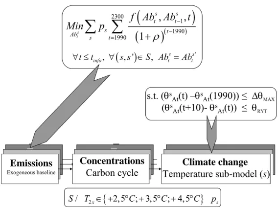
2. RESPONSE_Θ, a cost-efficiency optimal control integrated assessment model

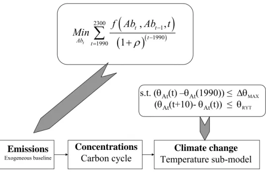
RESPONSE_Θ belongs to the RESPONSE model family (Ambrosi et al., 2003), a generic set of stochastic climate policy optimisation integrated assessment models. It includes a simple description of climate policy costs (baseline scenario and abatement cost function) and of the chain linking emissions to climate change through reduced-forms of carbon cycle and climate

dynamics. RESPONSE_Θ seeks to minimise the discounted sum of abatement costs (1) with

respect to two climate constraints (see Figure 1) 7_:

− one constraint on the magnitude of warming (2). ∆θ_MAX is set at +2 °C (in the central

case), which is close to the long-term climate policy goal stated by the European Union in 1996 and very recently reaffirmed with a formal statement coming just after the tenth Conference of the Parties to the Climate Convention: “the global average

[temperature] should not exceed the preindustrial level by more than 2 °C” (Council

of the European Union, 2004)8. Likewise the International Climate Change Taskforce

(2005) recommends a similar objective. This approach outlines environmental risks: by specifying such a constraint, or guardrail, it delimits a space inside which climate change impacts and their socio-economic repercussions are considered socially

tolerable9. Whether objective dangerous thresholds are clearly characterised (a drift of

the climate system, like the shutdown of the thermohaline circulation in the North Atlantic, is dangerous per se) or whether climate change entails impacts on a regional scale that are considered critical (for instance, the extinction of vulnerable ecosystems such as coral reefs or mountain vegetation, a disruption in monsoon cycles on the Indian subcontinent, warming over the Arctic, an increase in the risk of storm surges for Small Islands States). Numerous impact studies will provide who wishes to stick to such an absolute security approach with relevant clues. For instance, results from the

7 _{See the Appendix. A presentation of RESPONSE as well as its code (GAMS language) is given in Ambrosi}

(2004), downloadable at www.centre-cired.fr

8 _{Making an explicit reference to preindustrial times implies in fact a tighter constraint (1,5 °C since 1990)}

given the observed global warming in the past centuries.

9 _{Which does not mean, precisely, that a +2°C target could be regarded as safe. Warren’s review (2005) suggests}

indeed many impacts are not totally benign on a local scale, even for lower warming, but the elicitation of a target involves value judgments reflecting our concerns for different categories of impacts, our solidarity with vulnerable regions and with our descendants and our attitude towards risk.

Global Fast Track Assessment (Parry et al., 2001) suggest a comparable dangerous

threshold, with a sharp increase in the number of people at risk of water shortage once global mean temperature rise gets close to +2 °C. Besides, a recent report concludes to similar recommendations after an exhaustive review of impact studies, with multiple risks were global warming to venture beyond +2 or 3 °C (ECF, 2004).

− one constraint on the decadal rate of warming, ∆θRYT (3). Introducing such a constraint

puts the issue of impacts back in a dynamic perspective, with transient risks linked to the pace of climate change and of the deployment of its impacts. Very few information on this topic are available. Global disruptions of the climate system (such as the thermohaline circulation – Rahmstorf (2002)) are known to be sensitive to the rate of climate change beside its absolute magnitude. The risks which are characterised at best relate to ecosystems (Leemans and Eickhout, 2004; WWF, 2000). By analysing the ability of trees to migrate in response to climate fluctuations during the recent Quaternary, Krause et al. (1989) have recommended + 0.1 °C per decade as a maximum tolerable rate of warming. Leemans and van Vliet (2005) advocate even for 0.05 °C per decade safe guardrail! Those are very stringent constraints, especially with regard to the latest IPCC projection for the rate of warming: likely (probability between 0.66 and 0.9) between +0.1 and +0.2 °C per decade for the coming years (Houghton et al.(2001), SPM, p. 13).

The abatement cost function is taken from STARTS (Lecocq, 2000). Following these specifications, emissions reduction costs are represented as a backstop technology (initial

value: 1,100 US$.tC-1) with convex (quadratic) marginal costs. They incorporate an

autonomous technical change factor (costs decrease at a yearly constant rate of 1% but cannot decrease beyond 25% of their initial values) and the influence of socio-economic inertia as a cost-multiplier, through a multiplicative index which increases with the degree of socio-economic inertia (related to the average capital stocks turnover).

Baseline emissions (amount of CO2 emissions, both from fossil fuel use and land-use) come

from the marker scenario for the A1 SRES family, A1m (Nakicenovic, 2000). It corresponds to rather optimistic beliefs about the future. A1m is indeed the picture of a prosperous and generous world where economic growth is high with a considerable catch-up of developing countries, continuous structural change and rapid diffusion of more efficient technologies, three factors yielding to decreasing GHGs emissions as soon as 2050. A1m hypotheses could thus typically support beliefs which could justify a belated action since such a stance frequently appeals to

− either the argument of technical change: “it is better to invest in R&D in the energy

sector and/or research in climate change-related fields than to deep-cut fossil fuel emissions at once while alternative technologies are expensive and climate change consequences might prove ultimately benign”

− or the argument of development10_{: “developing countries are likely to be the main}

victims of climate change, which is almost in pipe for the next fifty years. Rather than curbing down GHGs emissions in industrialised countries whatever the costs, one should instead help LDCs in planning robust adaptation strategies and investing in the energy sector to lop their emissions peaks in the years to come. Even if climate change finally proves benign, it’s a no-regret option since it favours sustainable development”.

It is therefore relevant to examine how statements like “one should delay GHGs emissions

reduction efforts” are to be revised when using a proper precautionary approach based on the

same data.

We use the C-Cycle from DICE and RICE (Nordhaus and Boyer, 2000), a linear three-reservoir model (atmosphere, biosphere + surface ocean and deep ocean). Each three-reservoir is assumed to be homogenous (well-mixed in the short run) and is characterised by a residence time inside the box and corresponding diffusion rates towards the two other reservoirs (longer timescales). Carbon flows between reservoirs depend on constant transfer coefficients. GHGs

emissions (CO2 solely) accumulate in the atmosphere and they are slowly removed by

biospheric and oceanic sinks. Note however that the model accounts for the irreversible accumulation of part of the GHGs into the atmosphere: in 1000 years, there still remain, under

contemporary climatic conditions, some 13% of one ton CO2 emitted today (Siegenthaler and

Sarmiento, 1993).

To represent the evolution of global mean temperature, a set of two equations is used to describe its variation since pre-industrial times in response to additional human-induced

forcing: it is a perturbation model. CO2 is the only GHG modelled. Since the main issue is the

timing of abatement over the short run, we prioritise the description of the interaction between the atmosphere and the surface ocean neglecting the interactions with the deep ocean: the model describes the modification of the thermal equilibrium between atmosphere and surface ocean in response to anthropogenic greenhouse effect. Long-term climate dynamics is constrained by climate sensitivity. Three mechanisms are represented: the additional radiative

forcing in the atmosphere due to CO2 accumulation above its pre-industrial value, an

amplification/buffering of this perturbation through atmospheric feedbacks and a progressive thermal equilibrium atmosphere/surface ocean. We consider the uncertainty about climate sensitivity, the major contributor to the uncertainty in global warming projections for a given concentration pathway (other sources of uncertainty relate to, in order of importance, radiative forcing (esp. aerosols), ocean heat uptake and carbon cycle dynamics). The uncertainty regarding climate sensitivity is large, more than 3 °C, and persists since the second IPCC report: “The equilibrium climate sensitivity (…) was estimated to be between +1.5 °C and

+4.5 °C in the SAR. This range still encompasses the estimates from the current models in active use” (see Houghton et al. (2001), chp. IX, p. 561). At this time, Wigley and Raper

(2001) have proposed an ad hoc lognormal distribution, with a 90% confidence range from 1.5°C to 4.5°C. Since then, significant researches have been led to better characterise climate

sensitivity and quantify its accompanying uncertainty11 but this parameter is hard to constrain,

either from observations (because historical radiative forcing and ocean heat uptake data are fragile) (Andronova and Schlesinger, 2001; Forest et al., ; Gregory et al., 2002; Knutti et al., 2003, 2002; Frame et al., 2005) or from atmosphere-ocean global circulation models (because the parametrisations of some key processes such as cloud effects need improving) (Murphy et al., 2004; Stainforth et al., 2005). These studies have produced new estimates which remain concentrated over the +1.5 °C +4.5 °C range with a mean close to +3.5 °C but they indicate that one can not exclude much higher values, admittedly with low probabilities. To account for this uncertainty, we explore three values, centred around the mean estimate, {+2.5 °C ; +3.5 °C ; +4.5 °C } with the following probabilities {1/6; 2/3; 1/6} (close to the distribution obtained by Murphy et al. (2004)). To convey an idea of the consequences of this distribution

for decision, it means that to achieve a +2°C target with at least 80% confidence CO2

concentration must be stabilised at 450 ppm or below. To account for the uncertainty about

11

For a review of these studies, the methodologies followed, their limits and their results, see the National Academies (2003) or IPCC WGI (2004).

climate sensitivity (esp. the tail of the distribution for high values) and also for the various attitudes towards risk people will adopt in front of such fragile information given their personal concerns and their degree of risk aversion, we will test alternative distributions (see below), which convey a different weight to bad news (ie high climate sensitivity).

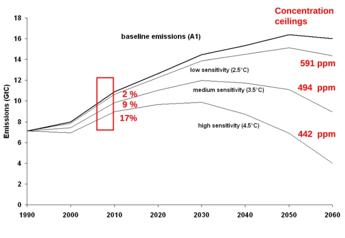
To conclude this presentation of RESPONSE_Θ, let us examine its results for a warming

threshold set at +2 °C (with no rate constraint for the moment). The uncertainty about climate sensitivity leads to very different optimal emissions trajectories (see Figure 2). It is therefore a crucial uncertainty for decision, notably for the decades to come: in 2010, mitigation efforts amount to 2, 9 or 17% of baseline emissions as climate sensitivity is low (+ 2.5 °C), medium (+ 3.5 °C) or high (+ 4.5 °C). Opting for a +2 °C temperature ceiling implies in fact to

stabilise long-term CO2 atmospheric concentration at a level all the more stringent as climate

sensitivity is high, respectively 591 ppm, 494 ppm and 442 ppm.

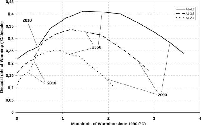
Let us now analyse the relative influence of both climate constraints, which approximate climate risks. To this aim, we have a look at baseline temperature trajectories for different values of climate sensitivity to detect at what time these constraints can bite and how their respective importance varies (Figure 3).

The diagram is to be read as follows: since global mean temperature is always increasing, we move with time along each curve from the left-hand side to the right-hand side; some dates have been written down to ease reading. The early kink is due to the fact that baseline emissions increase sharply as soon as 2000. The increase in global mean temperature is related to the magnitude and duration of forcing, that is to say to the atmospheric stock of

CO2. Given that this stock is ever-increasing (at least up to 2150), temperature is increasing as

well. Its rate however (look at the y-axis) depends on the increase in the forcing between two

periods of time. The latter is directly related to the increment of the atmospheric stock of CO2,

that is to say, apart from carbon cycle, to the time profile of emissions. As for the magnitude of the curves, it depends on the value of climate sensitivity.

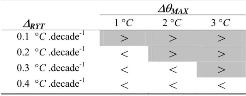
Beyond 2050 global mean temperature is increasing at a much smaller rate than in the first half of the 21st century because GHGs emissions begin to curb down as soon as 2050 in the baseline scenario. From now on to 2050 thus, the rate constraint bites at most, all the more as it is stringent and climate sensitivity is high. To slow down this acceleration, one must intensify mitigation efforts during the first part of the century. Results from the sensitivity analysis for short-term abatement are given in Table 1. These are close to the conclusions of

Tolerable Windows Approach et Safe landing Analysis (Metz et al. (2001), chap. X):

controlling the rate of climate change sets a significant constraint on GHGs emissions during

the first half of the 21st century, especially as this constraint is set at 0.1 or 0.2 °C per decade.

Sensitivity analyses provide useful information (above all, concerning extreme situations) but do not represent decision-making under uncertainty unless the decision criterion adopted is

Maximin or miniMax Regret (that is to say, criteria which do not use probability distributions

on the occurrence of future states of the world). For instance, using our former results, which short-term decision is optimal given that the uncertainty about climate sensitivity leads to recommendations varying from 2% to 17% in 2010? Furthermore, sensitivity analyses do not take into account learning, which introduces through sequential decision-making process flexibility over the very long time span of climate policies. Two important limits we now propose to overcome.

3. Optimal climate policy in the presence of uncertainty concerning climate sensitivity

To represent decision-making under uncertainty about climate sensitivity with learning, we

have altered RESPONSE_Θ in the following manner (Figure 4). Uncertainty about climate

sensitivity is discrete: we consider three possible states of the world (s) in which climate sensitivity may be equal to {+2.5 °C ; +3.5 °C ; +4.5 °C } with the corresponding ex ante

subjective probabilities or priors (pS) {1/6; 2/3 ; 1/6}. Learning is autonomous. Information

arrives at a fixed point in time ( tinfo ) : it can be available at the beginning of each decade in

the 21st century, with two polar cases, perfect information (tinfo =1990) and complete

uncertainty (tinfo =2300, the horizon of RESPONSE_Θ ).

The decision-maker adopts the best12 sequence of actions given that information on the ‘true’

state of the world will be available at tinfo : beyond this date, he can adapt the optimal

abatement profile to that information (three states of the world so three possible abatement trajectories); before this date, he has to adopt one common decision given subjective probabilities on the likelihood of the future states of the world and the date of disclosure of information. In numerical terms, the objective function (1a) is re-specified as the minimization of expected costs of abatement trajectories across the three states of the world, with respect to one constraint on the magnitude of warming (2) and one constraint on the decadal rate of warming (3). Sequential decision-making is captured through an additional constraint (1b) which imposes that, before the disclosure of information, decision variables be the same across all states of the world.

3.1 Under complete uncertainty, an attraction by the worst-case hypothesis with significant economic regrets

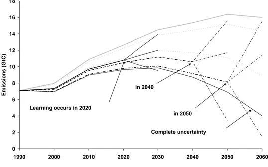
Let us first examine RESPONSE_Θ recommendations in the never learn case (tinfo =2300)13.

We can notice (Figure 5) that optimal emissions path totally sticks to the worst case hypothesis (climate sensitivity equal to +4.5 °C), generating thus significant economic regrets (i.e. investments in abatement technologies finally non necessary and often non-retrievable) if climate sensitivity ultimately turns out to have a lower value. In other words, results are similar to those obtained with a Maximin decision criterion which focuses only on the worst case. In a cost-effectiveness framework indeed, environmental constraints must be satisfied whatever the cost: as a consequence, one observes a complete attraction by the worst-case hypothesis, which corresponds to the lowest concentration ceiling (442 ppm).

3.2 The key role of learning: flexibility in short-term abatement efforts

However, if one takes into account an eventual learning in the future, short-term mitigation efforts may be relaxed, which reduces economic regrets. This effect is all the more pronounced as learning occurs early. For instance, abatement efforts in 2010 amount to 17% of baseline emissions in the never learn case and they gradually decrease to respectively 16, 12 and 11% (very close to the central case, climate sensitivity equal to +3.5 °C) as the information is available respectively in 2050, 2040 and 2020. These results are similar to the

12 _{Meaning here “the least expensive abatement trajectory which satisfies the environmental constraints”.} 13

Or, similarly, a situation where the decision-maker neglects the eventuality of future learning and takes his/her decision once for all.

conclusions reached by Ha Duong et al. (1997) in the context of the stabilisation of GHGs atmospheric concentrations: there exists indeed almost an equivalence between aiming at a temperature threshold in the presence of uncertainty on climate sensitivity and stabilising GHGs atmospheric concentrations at ceilings not known yet.

One must nonetheless notice one can not take for granted such information be soon available (Kelly et al., 2000; Leach, 2004): at least fifty years could be necessary to acquire from observation a reliable estimate of the value of climate sensitivity, which finally forces one to follow relatively stringent emissions pathways.

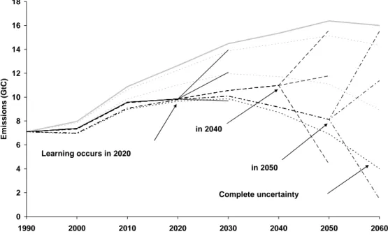
3.3 Significant short-term regrets with the rate constraint

But the rate constraint, even when not stringent, almost neutralises short-term benefits from learning. It implies indeed significant short-term mitigation efforts and deprives us from the flexibility allowed for by future learning (see Figure 6, with the rate constraint set at 0.3 °C per decade). In other words, in a context of uncertainty about climate sensitivity, the influence of the rate constraint on short-term decision is magnified because one must take into account the eventuality that climate sensitivity may be equal to + 4.5 °C, leading to a more intense and faster warming.

These conclusions are robust to the beliefs of the decision-maker, i.e. his/her subjective distribution of probabilities linked with the uncertainty on climate sensitivity. Beside a central belief, we have also tested a neutral one, as an interpretation of the Principle of insufficient reason (equiprobable distribution, mean equal to +3.5 °C: {1/3 ; 1/3 ; 1/3}), an optimistic one (left-skewed distribution, mean equal to +3 °C :{2/3 ; 1/6 ; 1/6}) and lastly, a pessimistic one (right-skewed distribution, mean equal to +4 °C : {1/6 ; 1/6 ; 2/3}). Whatever the prior of the decision-maker, the optimal abatement rate in 2020 (learning occurring in 2020) amounts to about 22.0 % of baseline emissions, which is very close to the worst-case hypothesis under certainty at the same time (23.6 %) and almost twice the optimal abatement effort in the central case at the same time (12.8 %).

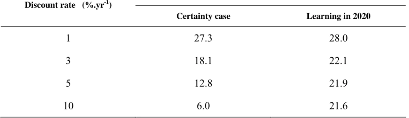
These results are also robust to discounting, which is – in the certainty case – the most decisive socio-economic parameter for decision, with the effect to pass on emissions reduction efforts from the present generation to future generations (see Table 2, left column). In the certainty case, the optimal abatement rate differs widely depending on the value of the discount rate (from 6 to 27% as the discount rate decreases from 10 to 1% a year): recall that in a cost-efficiency framework, a high discount rates reduces the discounted value of future costs, which favours postponing for some decades the bulk of mitigation efforts. In the learning case (see Table 2, right column), the optimal abatement rate is systematically greater than the optimal rate in the certainty case. Above all, the influence of the discount rate is much less important than before: it still favours a belated action (the mitigation effort decreases as the discount rate increases) but for 3, 5 and 10% a year the optimal abatement rates are almost comparable and only the optimal response for a 1% a year discount rate singles out .

So, the results from this analysis demonstrate that, in the presence of uncertainty, the relative

influences established through the sensitivity study of RESPONSE_Θ are still valid even if

they are no longer as pronounced. Whereas in the certainty case sharp controversies may arise over the choice of a correct value for the discount rate since the optimal abatement rate may

accordingly vary by a factor of 4, conflicting views concerning this parameter are not anymore as decisive when following a sequential decision approach, especially if the debate focuses around values such as 3-5 % a year (a plausible range given the baseline scenario growth rate and standard assumptions regarding the economic agent preferences), which unanimously leads to a mitigation rate of 22%.

The uncertainty concerning climate sensitivity is thus crucial: it leads to significant short-term mitigation efforts all the more as the arrival of information regarding this parameter is belated or under the influence of the rate constraint (be it stringent or not). In this context, a +2 °C objective could lead to rather stringent policy recommendations for the coming decades and might prove unacceptable. These results are insensitive to the distribution of climate sensitivity and to the choice of the discount rate. The date of learning and the rate constraint are on the other hand key-parameters for short-term decision.

Alike the constraint on the magnitude of warming, the rate constraint is notably unknown yet: some will argue for a very tight constraint but others will advocate much looser a constraint, be they quite optimistic about our future adaptive capacities or less concerned by endangered ecosystems. Some time might therefore be needed before a social consensus be reached or major breakthroughs in climate or impacts science help in defining unambiguously a “dangerous interference with the climate system” or in better quantifying climate sensitivity. In view to rank out the relative influence of these three uncertainties on short-term decision, we next compute the value of information associated with each of these three parameters.

4. A ranking of uncertainties using the value of information

The value of information, Expected Value of Perfect Information (EVPI), measures the opportunity to possess a piece of information when making a decision. Since we place ourselves in a dynamic perspective, we compute EVPI as the maximal willingness to pay to obtain today this piece of information rather than waiting a later time. EVPI is classically defined as the difference between the expected value of the objective function in the “Act then Learn” case (a policy must be adopted before the disclosure of information) and in the “Learn then Act” case (the value of the parameter is known from the outset and a policy is adopted

accordingly). Following RESPONSE_Θ notations, we have :

(

)

(

)

(

₍

₎

)

ATL t t ATL t t LTA t LTA t

info s t s t

s t s t

Learn then Act policy Act then Learn policy

f Ab Ab t f Ab Ab t EVPI t p p ρ ρ − − − − = = ⎛ _{⎞ ⎛ ⎞} ⎜ _{⎟ ⎜ ⎟} = − ⎜ ₊ ⎟ ⎜_{⎝ +} ⎟_⎠ ⎝_14444444

∑ ∑

∑ ∑

with AbSATL(t_info),t optimal course of abatement, the state of the world, s, being disclosed

at time tinfo.

AbSLTA,t optimal course of abatement in the certainty case, the state of the world

being s.

EVPI allows today’s decision-maker to rank out the relative importance of a set of uncertain

parameters. For instance, EVPI ad infinitum, EVPI(2300), reveals the magnitude of the regrets at never possessing a definitive information to incorporate it in the decision process.

EVPI(2300) measures the costs of complete uncertainty and the amount one is willing to pay

precautionary climate policies. Moreover, the time profile of EVPI shows the opportunity to accelerate the reduction of uncertainties: if EVPI increases sharply between two points in time, it is then vital for today’s decision-maker to get the information at the beginning of this period.

We explore the following sets for climate sensitivity {+2.5 °C ; +3.5 °C ; +4.5 °C}, the magnitude constraint {+1 °C ;+2 °C ;+3 °C } and the rate constraint {0.1 °C per decade ; 0.2 °C per decade ; 0.3 °C per decade }. The accompanying subjective probability distribution is the following: {1/6 ; 2/3 ; 1/6}.

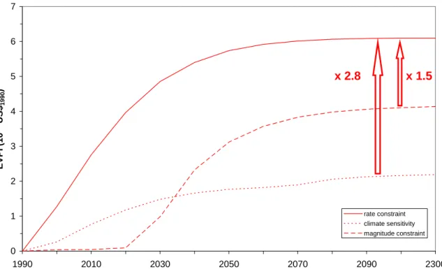
Once again, the prominent influence of the rate constraint is confirmed (Figure 7).

Unquestionably, it exhibits the highest value of information: the fastest increase (in 2020, more than 60% of its value ad infinitum ; almost 90% in 2040, 20 years later) and the highest value ad infinitum (2.8 times greater than EVPI for climate sensitivity and 1.5 times greater than EVPI for the magnitude constraint). The respective dominances of the other two parameters vary with time: EVPI for climate sensitivity is greater than EVPI for the magnitude constraint until 2035 and the situation then reverses (in 2100, EVPI for the magnitude constraint is greater than EVPI for climate sensitivity by a factor of 1.8). With respect to their value ad infinitum, the value of information attached to climate sensitivity increases faster (in 2020, more than 50% of its value ad infinitum, almost 70% 10 years later, in 2030) whereas the value of information for the magnitude constraint increases sharply from 2020 onwards (in 40 years, from 2020 to 2060, it grows by more than 80%).

There exists thus a high opportunity cost to know before 2040 the scientific-objective or socially acceptable values for the rate constraint, climate sensitivity and the magnitude constraint, and on a closer horizon (between now and 2020) to know the first two parameters. Beyond this opportunity window, there still exists of course a benefit to discover the values for these parameters but with regard to short-term flexibility in the abatement effort, the late acquisition of information is not that decisive (one must indeed follow a very stringent emissions pathway, if not stick to the worst case hypothesis).

These results qualitatively hold for alternative values of the discount rate (Figure 8): prominent role of the rate constraint (highest value and fastest increase at least for the next 40 years), climate sensitivity (second highest value for the next 30 years) and magnitude constraint (sharp increase from 2020 onwards). Interestingly, EVPI makes clear the balance of short- and long-term induced by the choice of discount rate. In a world with high discounting, mitigation efforts tend to be postponed at the most. The uncertainty regarding the rate constraint or climate sensitivity (through its synergy with the rate constraint on short-term) is thus particularly crucial on short-term since it implies significant abatement rates in the coming decades one would prefer to delay. Conversely, in a world with low discounting, mitigation efforts are spread evenly across time and long-term horizon is conveyed more weight. As a result, uncertainties that are more pregnant on long-term are also given consideration seen from today: the value of information associated with the magnitude constraint (related to the atmospheric stock of carbon and to climate sensitivity) increases gradually with time and on long-term becomes the highest EVPI.

These results qualitatively hold for priors of the decision-maker (Figure 9). The relative importance of the three uncertainties remains unaltered but the scale of the EVPIs decreases as the decision-maker becomes more pessimistic. This is due to the fact that in an optimistic view, the decision-maker must accept significant abatement efforts as long as the uncertainties

are not reduced even if the worst-case is conveyed a low weight: any information is therefore valuable since it makes possible to escape from the attraction by the (less likely) worst-case. As for defining proxies of climate risks based on the global mean temperature, the most crucial informations relate first, to the critical rate of climate change socially acceptable – that is to say a transient characteristic of risks – and second, to the critical magnitude of climate change – that is to say a long-term constraint.

5. Conclusion

Our results demonstrate that there exists a high opportunity cost to know before 2030 the value of climate sensitivity in view to mitigate to some extent the significant economic regrets that are concomitant with a precautionary policy in the presence of uncertainty about this parameter. One can not take for granted such information be soon available (at least fifty years could be necessary), which finally forces one to follow relatively stringent emissions pathways. In this context, a +2 °C might thus be considered unacceptable.

Furthermore, we find that when stepping from an abstract definition of climate risks based on desirable concentration ceilings to a more palpable definition based on long-term global protection (magnitude of climate change) and transient protection (rate of climate change), a precautionary climate policy – even if both long-term objectives, concentration ceiling or warming threshold, are equivalent - implies more short-term abatement efforts as rate constraint bites, which is the case in the presence of uncertainty regarding climate sensitivity for values as high as 0.3 °C per decade. We besides show that the uncertainty about the rate constraint is even more important for short-term decision than the uncertainty about climate sensitivity or magnitude of warming. This means that the critical rate of climate change, i.e. a transient characteristic of climate risks, matters much more than the long-term objective of climate policy, i.e. the critical magnitude of climate change. Therefore, research should be aimed at better characterising climate change risks in view to help decision-makers to agree on a safe guardrail to limit the rate of global warming.

Further perspectives of this research involve the improvement of the carbon-climate sub-models (multigas, ocean-heat uptake, climate-carbon feedback) in view to assess in the same framework and following a similar approach, the relative importance for decision of these mechanisms which are uncertain yet.

6. Bibliographical references

Alcamo, J. and E. Kreileman. 1996. "Emissions scenarios and global climate protection." Global Environmental Change, 6:4, pp. 305-34.

Ambrosi, Ph. 2004. "Amplitude et calendrier des politiques de réduction des émissions en réponse aux risques climatiques: leçons des modèles intégrés." Economie de l'environnement. Ecole des Hautes Etudes en Sciences Sociales (EHESS): Paris.

Ambrosi, Ph., J.C. Hourcade, S. Hallegatte, F. Lecocq, P. Dumas, and M. Ha Duong. 2003. "Optimal control models and elicitation of attitudes towards climate damages." Environmental Modeling and Assessment, 8:3, pp. 133-47.

Andronova, N.G. and M. E. Schlesinger. 2001. "Objective estimation of the probability density function for climate sensitivity." Journal of Geophysical Research, 106:D19, pp. 22605-11.

Böhringer, C., A. Löschel, and T.F. Rutherford. 2005. "Efficiency Gains from “What”-Flexibility in Climate Policy - An Integrated CGE Assessment." The Energy Journal, forthcoming.

Caldeira, K., A.K. Jain, and M.I. Hoffert. 2003. "Climate sensitivity uncertainty and the need for energy without CO2 emission." Science, 299:5615:28 March 2003, pp. 2052-54.

Council of the European Union. 2004. "Press Release: 2632nd Council Meeting." Council of the European Union: Brussels (Belgium).

ECF. 2004. "What is dangerous climate change?-Initial Results of a Symposium on Key Vulnerable Regions, Climate Change and Article 2 of the UNFCCC." ECF and PIK.

den Elzen, M.G.J. and M. Meinshausen. 2005a. "Emission implications of long-term climate targets." Avoiding Dangerous Climate Change: Exeter (UK).

den Elzen, M.G.J. and M. Meinshausen. 2005b. "Meeting the EU 2°C climate target: global and regional emission implications." 44. Netherlands Environemental Assessment Agency (MNP associated the RIVM): Bilthoven (the Netherlands).

Frame, D. J., B.B.B. Booth, J.A. Kettleborough, D. A. Stainforth, J. M. Gregory, M. Collins, and M. R. Allen. 2005. "Constraining climate forecasts: The role of prior assumptions." Geophysical Research Letters, 32:L09702, pp. doi:10.1029/2004GL022241.

Forest, C. E., P. H. Stone, A. P. Sokolov, M. R. Allen, and M. D. Webster. 2002. "Quantifying uncertainties in climate system properties with the use of recent climate observations." Science, 295:5552, pp. 113-17.

Gregory, J. M. , R. J. Stouffer, S. C. B. Raper, P. A. Stott, and N. A. Rayner. 2002. "An Observationally Based Estimate of the Climate Sensitivity." Journal of Climate, 15:22, pp. 3117–21.

Ha Duong, M., M. Grubb, and J.C. Hourcade. 1997. "Influence of socioeconomic inertia and uncertainty on optimal CO2-emission abatement." Nature, 390, pp. 270-74.

Hammitt, J.K., R. J. Lempert, and M. E. Schlesinger. 1992. "A sequential-decision strategy for abating climate change." Nature, 357, pp. 315-18.

Hare, B. and M. Meinshausen. 2004. "How much warming are we committed to and how much can be avoided?" 45. Potsdam Institute for Climate Impact Research (PIK): Potsdam (Germany).

Hitz, S. and J. Smith. 2004. "Estimating global impacts from climate change," in The benefits of climate change policies: analytical and framework issues. J. Corfee-Morlot and S. Agrawala eds. Paris: OCDE/OECD, pp. 31-82.

Houghton, J. T., Y. Ding, D.J. Griggs, P.J. Noguer, P.J. van der Linden, X. Dai, K. Maskell, and C.A. Johnson eds. 2001. Climate change 2001: the scientific basis. Contribution of Working Group I to the Third Assessment Report of the Intergovernmental Panel on Climate Change. Cambridge (UK&US): Cambridge University Press. International Climate Change Taskforce. 2005. "Meeting the Climate Challenge: Recommendations of the International Climate Change Taskforce."

IPCC WGI. 2004. "Workshop on Climate Sensitivity." 177. IPCC: Paris (France).

Kelly, D., C. D. Kolstad, M. E. Schlesinger, and N.G. Andronova. 2000. "Learning About Climate Sensitivity From the Instrumental Temperature Record."

Knutti, R., T.F. Stocker, F. Joos, and G.-K. Plattner. 2003. "Probabilistic climate change projections using neural networks." Climate Dynamics, 21, pp. 257-72.

Knutti, R., T.F. Stocker, F. Joos, and G.-K. Plattner. 2002. "Constraints on radiative forcing and future climate change from observations and climate model ensembles." Nature, 416:6882, pp. 719 - 23.

Krause, F., W. Bach, and J. Koomey. 1989. "Energy policy in the greenhouse (Final report)." Vol. volume 1: From warming fate to warming limit: benchmarks for a global climate convention. International Project for Sustainable Energy Paths (IPSEP): El Cerrito (CA).

Kriegler, E. and T. Bruckner. 2004. "Sensitivity Analysis of Emissions Corridors for the 21st Century." Climatic Change, 66:3, pp. 345-87.

Leach, A. 2005. "The Climate Change Learning Curve." 33. HEC Montreal: Montreal (Canada).

Leemans, R. and A. van Vliet. 2005. "Responses of Species to Changes in Climate Determine Climate Protection Targets." Avoiding Dangerous Climate Change: Exeter (UK).

Leemans, R. and B. Eickhout. 2004. "Another reason for concern: regional and global impacts on ecosystems for different levels of climate change." Global Environmental Change, 14, pp. 219-28.

Lecocq, F. 2000. "Distribution spatiale et temporelle des coûts des politiques publiques sous incertitudes: théorie et pratique dans le cas de l'effet de serre." Sciences de l'environnement. Ecole Nationale du Génie Rural, des Eaux et Forêts (ENGREF): Paris.

Lempert, R. J. 2002. "A New Decision Sciences for Complex Systems." Proceedings of the National Academy of Sciences (PNAS), 99:suppl. 3, pp. 7309-13.

Lempert, R. J. and M.E. Schlesinger. 2001. "Climate-Change Strategy Needs to be Robust." Nature, 412:26 July 2001, pp. 375.

Lempert, R. J., M. E. Schlesinger, and J.K. Hammitt. 1994. "The impact of potential abrupt climate changes on near-term policy choices." Climatic Change, 24, pp. 351-76.

Lomborg, B. 2001. The Skeptical Environmentalist: measuring the real state of the world. Cambridge (UK&US): Cambridge University Press.

McCarthy, J. J., O. F. Canziani, N. A. Leary, D. J. Dokken, and K. S. White eds. 2001. Climate Change 2001: Impacts, adaptation and vulnerability. Contribution of Working Group II to the Third Assessment Report of the Intergovernmental Panel on Climate Change. Cambridge (UK & US): Cambridge University Press.

Manne, A.S. and R. Richels. 2005. "Global Climate Decisions under Uncertainty." International Energy Workshop 2005 (IEW 2005): Kyoto (Japan).

Mastrandea, M.D. and S.H. Schneider. 2004. "Probabilistic Integrated Assessment of ‘Dangerous’ Climate Change." Science, 304:23 April, pp. 571-75.

Meehl, G. A., M.A. Washington, W.D. Collins, J.M. Arblaster, A. Hu, L.E. Buja, W.G. Strand, and H. Teng. 2005. "How Much More Global Warming and Sea level Rise?" Science, 307:5716, pp. 1769-72.

Meinshausen, M. 2005. "On the risk of overshooting +2°C." Avoiding Dangerous Climate Change: Exeter (UK). Metz, B., D. Ogunlade, R. Swart, and J. Pan eds. 2001. Climate Change 2001: Mitigation. Contribution of Working Group III to the Third Assessment Report of the Intergovernmental Panel on Climate Change. Cambridge (UK & US): Cambridge University Press.

Murphy, J. M. , D. M. H. Sexton, D N. Barnett, G. S. Jones, M. J. Webb, M. Collins, and D. A. Stainforth. 2004. "Quantification of modelling uncertainties in a large ensemble of climate change simulations." Nature,

Nakicenovic, N. ed. 2000. Special Report on Emissions Scenarios: a special report of Working Group III of the Intergovernmental Panel on Climate change. Cambridge (UK&US): Cambridge University Press.

the National Academies. 2003. "Estimating Climate Sensitivity: Report of a workshop." 41. Steering committee on Probabilistic Estimates of Climate Sensitivity, Board on Atmospheric Sciences and Climate, Division of Earth and Life Studies, the National Academies: Washington D.C.

Nordhaus, W. and J. G. Boyer. 2000. Warming the world: Economics models of Climate Change. Cambridge (MA, USA): MIT Press.

O'Neill, B. C. and M. Oppenheimer. 2004. "Climate change impacts are sensitive to the concentration stabilisation path." PNAS, 1001:47, pp. 16411-17.

Parry, M., N. Arnell, McMichael T., R. Nicholls, P. Martens, S. Kovats, M. Livermore, C. Rosenzweig, A. Iglesias, and G. Fischer. 2001. "Millions at Risk: defining critical climate change threats and targets." Global Environmental Change, 11, pp. 181-83.

Rahmstorf, S. 2002. "Ocean circulation and climate during the past 120,000 years." Nature, 419:12 September 2002, pp. 207-14.

Richels, R., A.S. Manne, and T.M.L. Wigley. 2004. "Moving Beyond Concentrations: the Challenge of Limiting Temperature Change." AEI-Brookings joint Center for Regulatory Studies.

Schelling, T.C. 1992. "Some economics of global warming." American Economic Review, 82:1, pp. 1-14.

Schneider, S.H. and S.L. Thompson. 1981. "Atmospheric CO2 and climate: importance of the transient

response." Journal of Geophysical Research, 86, pp. 3135-47.

Siegenthaler, U. and J. L. Sarmiento. 1993. "Atmospheric carbon dioxide and the ocean." Nature, 365:6442, pp. 119-25.

Stainforth, D. A., T. Aina, C. Christensen, M. Collins, N. Faull, D. J. Frame, J. A. Kettleborough, S. Knight, A. Martin, J. M. Murphy, C. Piani, D. Sexton, L. A. Smith, R. A. Spicer, A. J. Thorpe, and M. R. Allen. 2005. "Uncertainty in predictions of the climate response to rising levels of greenhouse gases." Nature, 433:7024. Swart, R., M. Berk, M. Janssen, E. Kreileman, and R. Leemans. 1998. "The safe landing approach: risks and trade-offs in climate change," in Global change scenarios of the 21st century: results from the IMAGE 2.1 Model. J. Alcamo, R. Leemans and E. Kreileman eds. Oxford (UK): Pergamon/Elsevier Science, pp. 193-218. Toth, F.L., T. Bruckner, H.-M. Füssel, M. Leimbach, and G. Petschel-Held. 2003 a. "Integrated Assessment of Long-term Climate Policies: Part 1 - Model Presentation." Climatic Change, 56:1-2, pp. 37-56.

Toth, F.L., T. Bruckner, H.-M. Füssel, M. Leimbach, and G. Petschel-Held. 2003 b. "Integrated Assessment of Long-term Climate Policies: Part 2 - Model Results and Uncertainty Analysis." Climatic Change, 56:1-2, pp. 37-56.

UNFCCC. 1992. "United Nations Framework Convention on Climate Change (UNFCCC)."

Warren, R. 2005. "Impacts of Global Climate Change at Different Annual Mean Global Temperature Increases." Avoiding Dangerous Climate Change. Cambridge University Press (UK): Exeter (UK).

Wigley, T.M.L. 2005. "The Climate Change Commitment." Science, 307:5716, pp. 1766-69.

Wigley, T.M.L. and S. C. B. Raper. 2001. "Interpretation of high projection for global-mean warming." Science, 293:5529, pp. 451-54.

WWF. 2000. "Global Warming and Terrestrial Biodiversity Decline." World Wide Fund for Nature (WWF): Gland (Switzerland).

Yohe, G., N.G. Andronova, and M. E. Schlesinger. 2004. "To Hedge or Not Against an Uncertain Climate Future?" Science, 306:15 October 2004, pp. 416-17.

Appendix: RESPONSE, a stochastic climate policy optimisation integrated assessment model

A.1 Baseline growth scenario and exogenous related data (income and population)

All experiments are based on the SRES A1m scenario which has been computed by NIES (National Institute for Environmental Studies, Japan) with the AIM model (Asian Pacific Integrated Model) (Nakicenovic, 2000). Beyond 2100, emissions are computed on the basis of a simple relationship linking the decadal growth rate of emissions, the decadal growth rate of income, the autonomous improvement of energy efficiency and an autonomous trend in the decarbonisation of energy. In 2150, emissions are below 5 GtC a year and almost inexistent in 2200. On the whole, the total amount of carbon emitted reaches 2077 GtC (more than 2.7 times the atmospheric carbon content in 1980).

A.2 Specification of abatement cost function We use the following abatement cost function:

(

)

(

)

with: f(Abt,Abt-1,t) total cost of mitigation measures at time t (trillion US$)

BK initial marginal cost of backstop technology (thousand US$.tC-1)

PTt technical change factor

γ(Abt,Abt-1) socio-economic inertia factor

emt baseline CO2 emissions at time t (GtC)

Abt abatement rate at time t (% of baseline emissions)

Under these specifications, marginal costs of abatement are convex (quadratic). This is consistent with assumptions by experts and the results of technico-economic models. Note that f(.) does not allow for so-called no-regret potential.

BK stands for the initial marginal cost of backstop technology, i.e. the carbon free-technology

which would enable to completely reduce GHGs emissions were it to be substituted to current existing energy systems. Its value depends on a set of assumptions regarding its nature (windpower, nuclear …), its development date, its penetration rate and technical change.

Given our own assumptions on technical change, we retain an initial 1,100 US$.tC-1 _cost.

PTt captures the influence of autonomous technical change on abatement costs. It translates

the decrease of the costs of carbon-free technology over time, but the improvement of energy intensity which is already taken into account in the baseline. We assume that the costs of abatement technologies decrease at a constant 1% per year rate but we assume costs cannot

decrease beyond 25% of their initial values. PTt thus take the form below (which leads to an

ultimate cost of 275 US$.tC-1)

0.01

0.25 0.75 t t

PT _{= +} e− δ

where δ is the time step of the model (10 years)

γ(Abt,Abt-1) captures the influence of socio-economic inertia as a cost-multiplier (transition

costs between a more and a less carbon-intensive economic structure). γ(.) is a multiplicative

given threshold τ between two consecutive periods. But it increases linearly with the speed of

variation of abatement rate when this rate is higher than τ, i.e. the annual turnover of

productive capital below which mitigation policies do not lead to premature retirement of

productive units. Here τ is set to 5% per year (average capital stocks turnover of 20 years).

(

)

A.3 Three-reservoir linear carbon-cycle model

We use the C-Cycle of Nordhaus and Boyer (2000), a linear three-reservoir model (atmosphere, biosphere + surface ocean and deep ocean). Each reservoir is assumed to be homogenous (well-mixed in the short run) and is characterised by a residence time inside the box and corresponding mixing rates with the two other reservoirs (longer timescales). Carbon

flows between reservoirs depend on constant transfer coefficients. GHGs emissions (CO2

solely) accumulate in the atmosphere and they are slowly removed by biospheric and oceanic sinks.

The dynamics of carbon flows is given by is given by:

1 1 1 . (1 ) t t t trans t t t t A A . t B C B Ab em O O δ + + + ⎛ ⎞ ⎛ ⎞ ⎜ ⎟₌ ⎜ ⎟_{+ −} ⎜ ⎟ ⎜ ⎟ ⎜ ⎟ ⎜ ⎟ ⎝ ⎠ ⎝ ⎠ u ⎟ ⎟

with At carbon contents of atmosphere at time t (GtC)

Bt carbon contents of upper ocean and biosphere at time t (GtC)

Ot carbon contents of deep ocean at time t (GtC)

Ctrans net transfert coefficients matrix

u column vector (1,0,0)

As such, the model has a built-in ten-year lag between CO2 emissions and CO2 accumulation

in the atmosphere, which reflects the inertia in C-cycle dynamics. Nordhaus calibration on existing carbon-cycle models gives the following results (for a decadal time step):

0.66616 0.27607 0 0.33384 0.60897 0.00422 0 0.11496 0.99578 trans C ⎛ ⎞ ⎜ = ⎜ ⎜ ⎟ ⎝ ⎠ initial conditions (GtC): ₁₉₉₀ 758 793 19 230 C ⎛ ⎞ ⎜ ⎟ = ⎜ ⎟ ⎜ ⎟ ⎝ ⎠

The main criticism which may be addressed to this C-cycle model is that the transfer coefficients are constant. In particular, they do not depend on the carbon content of the reservoir (e.g. deforestation hindering biospheric sinks) nor are they influenced by ongoing climatic change (eg positive feedbacks between climate change and carbon cycle).

A.4 The reduced-form climate model

This model is very close to Schneider and Thompson’s two-box model (Schneider and Tompson, 1981). A set of two equations is used to describe global mean temperature variation (eq. 2) since pre-industrial times in response to additional human-induced forcing (eq. 1). More precisely, the model describes the modification of the thermal equilibrium between

atmosphere and surface ocean in response to anthropogenic greenhouse effect. Calibration was carried out with H. Le Treut (IPSL) from data kindly provided by P. Friedlingstein (IPSL). All specifications correspond to decadal values, which is the time step of the model.

Radiative forcing equation:

2 log ( ) log 2 t PI X M M F t F ⎛ ⎞ ⎜ ⎟ ⎝ = ⎠ (1)

with Mt CO2 atmospheric concentration at time t (ppm)

F(t) radiative forcing at time t (W.m-2)

MPI CO2 atmospheric concentration at pre-industrial times, set at 280 ppm.

F2X instantaneous radiative forcing for 2x MPI, set at 3.71 W.m-2.

Temperature increase equation:

1 2 1 2 1 3 3 ( 1) 1 ( ) ( ) ( ) ( 1) 1 ( ) 0 At At Oc Oc t t F t t t θ σ λ σ σ σ θ σ θ σ σ θ ⎧⎡ + ⎤ ⎡ − + ⎤ ⎡ ⎤ ⎡ ⎤ ⎪ _{= +} ⎨⎢ ₊ ⎥ ⎢ ₋ ⎥ ⎢ ⎥ ⎢ ⎥ ⎪⎣ ⎦ ⎣ ⎦ ⎣ ⎦ ⎣ ⎦ ⎩ (2)

with θAt(t) global mean atmospheric temperature rise wrt pre-industrial times (°C)

θOc(t) global mean oceanic temperature rise wrt pre-industrial times (°C)

λ climate response parameter (C-1.W.m-2)

σ1 transfer coefficient (set at 0.479 C.W-1.m2)

σ2 transfer coefficient (set at 0.109 C-1.W.m-2)

σ3 transfer coefficient (set at 0.131).

Climate sensitivity (T2x) is given by T2x= F2X / λ. We assume that uncertainty is mainly due to

uncertainty on (atmospheric) climate feedbacks process (represented by λ) rather than

uncertainty on F2X. A high climate response parameter will lead to low climate sensitivity. We

explore three values for climate sensitivity and λ is set accordingly to F2x/T2X see following

table:

State of the World LOW CENTRAL HIGH Climate sensitivity (T2x) 2.5 °C 3.5 °C 4.5 °C

Ex ante subjective probability (ps) 1/6 2/3 1/6

λ 1.48 1.06 0.82

A.5 Numerical resolution

To avoid boundary effects, we do not specify terminal conditions in 2100 but set the time horizon of the model at 2300. The model is run under the GAMS-MINOS non-linear solver. Code is available from the author on request.

Emissions

Exogeneous baseline

Concentrations

Carbon cycle Temperature sub-modelClimate change

(

)

(

)

,

,

1

f Ab Ab

t

Min

ρ

∑

+

9 % 17% 2 % 591 ppm 494 ppm 442 ppm Concentration ceilings

Figure 2. Sensitivity of optimal emissions trajectories to climate sensitivity – results from RESPONSE_Θ.

0 0,05 0,1 0,15 0,2 0,25 0,3 0,35 0,4 0,45 0 1 2 3 4

Magnitude of Warming since 1990 (°C)

D ecad al rate o f Warmin g (° C /d ecade) A1-4,5 A1-3,5 A1-2,5 2010 2050 2090 2010

Figure 3. Magnitude of warming (since 1990) vs. Decadal rate of warming in the baseline scenario for three values of climate sensitivity.

∆θ

∆

_>

_>

_>

_<

_>

_>

_{< < >}

< < <

To be read as follows : « > » means that the influence of the rate constraint dominates the influence of the magnitude constraint for short-term decision (up to 2050) and « < », the opposite.

Table 1. Relative influence of the climate constraints on the abatement rate during the 1st half of the 21st century.