Publisher’s version / Version de l'éditeur:
Vous avez des questions? Nous pouvons vous aider. Pour communiquer directement avec un auteur, consultez la
première page de la revue dans laquelle son article a été publié afin de trouver ses coordonnées. Si vous n’arrivez pas à les repérer, communiquez avec nous à PublicationsArchive-ArchivesPublications@nrc-cnrc.gc.ca.
Questions? Contact the NRC Publications Archive team at
PublicationsArchive-ArchivesPublications@nrc-cnrc.gc.ca. If you wish to email the authors directly, please see the first page of the publication for their contact information.
https://publications-cnrc.canada.ca/fra/droits
L’accès à ce site Web et l’utilisation de son contenu sont assujettis aux conditions présentées dans le site
LISEZ CES CONDITIONS ATTENTIVEMENT AVANT D’UTILISER CE SITE WEB.
Proceedings of the 4th U.S. National Conference on Earthquake Engineering, 3, pp. 95-104, 1990
READ THESE TERMS AND CONDITIONS CAREFULLY BEFORE USING THIS WEBSITE. https://nrc-publications.canada.ca/eng/copyright
NRC Publications Archive Record / Notice des Archives des publications du CNRC :
https://nrc-publications.canada.ca/eng/view/object/?id=f6cb1098-98a2-4076-bed8-894508c50fa7 https://publications-cnrc.canada.ca/fra/voir/objet/?id=f6cb1098-98a2-4076-bed8-894508c50fa7
NRC Publications Archive
Archives des publications du CNRC
This publication could be one of several versions: author’s original, accepted manuscript or the publisher’s version. / La version de cette publication peut être l’une des suivantes : la version prépublication de l’auteur, la version acceptée du manuscrit ou la version de l’éditeur.
Access and use of this website and the material on it are subject to the Terms and Conditions set forth at Effect of location of transmitting boundary on seismic hydrodynamic pressures on gravity dams
-
no. 1665 National Research Conseil natlonal
c. 2
I
*I
Council Canada de recherches Canada BLDG Institute for --- - lnstitut de Research in recherche en Construction constructionEffect of Location of Transmitting
Boundary on Seismic Hydrodynamic
Pressures on Gravity Dams
by Alexander M. Jablonski
Appeared in the
Proceedinas of the Fourth U.S. National Conference on ~afihquake Engineering
May 20-24,1990 Vol. 3, p. 95-104 (I RC Paper No. 1665)
Reprinted with permission from the
Earthquake Engineering Research Institute NRCC 32334 I N R C
-
CISTI I R C L I B R A R YI
BIBLIOTHEQUE
I R C C N ~ C - ICISTI
L'auteur utilise la mCthode &s Quations intCgrales @I) constantes pour &terminer l'effet & l'emplacement d'une limite & transmission sur les pressions hydrodynamiques sismiques dans un dservoir d'eau.
Jl
se serth
cette fin d'un d l e rnathematique 2D d'unsysttxne bmage-dservoir-fonhtion. Les dsultats &&lent que la g6omCtrie de la partie M e du r6servoir est
un
facteur dhminant pour ce qui est &s pressions hydrodynamiques s'exeqant sur les barrages, l'emplacement cle la limite & transmission dans le dservoir -ant la ghm6mede
cette partie. Dans le casdes
dservoirs presque mtangulaires, les dsultats de l'utilisation de la &pendent moins de l'emplacement. L'auteur a aussi CvaluC d'auaes facteurs : le nombre d'C1Cnments tmployCs pour modtliser la limite &transmission, le n o m h total d'ClCments et la longueur & lYClCment relativement
B
la pluscourte longueur #on& induite dans le dsemoir. J
EFFECT OF LOCATION OF TRANSMITTING BOUNDARY ON SEISMIC HYDRODYNAMIC PRESSURES ON GRAVITY DAMS
Alexander M. Jablonski I
ABSTRACT
The constant boundary element method is used to assess the effect of the location of a transmitting boundary on seismic hydrodynamic pressures in a water reser- voir. A 2D mathematical model of a dam-reservoir-foundation system is used. The results indicate that the geometry of the finite part of the reservoir is a gov- erning factor of hydrodynamic pressures acting on dams, where the location of the transmitting boundary changes the geometry of that part. For almost rectangular reservoirs the
BEM
results are less dependent on the location. Additional factors evaluated are the number of elements used to model the transmitting boundary, the overall number of elements and the length of the element with respect to the induced shortest wave length in the reservoir.INTRODUCTION
A concrete gravity dam is designed to be stable under its own load as well as hydro- static and hydrodynamic water pressures. The dam cross-section is usually kept constant throughout the length of the dam. In this case a
2D
geometrical model may be sufficient.Extensive research on the seismic response of gravity dam-reservoir-foundation sys- tems has been pursued during the last decade. The finite element method and boundary element method have been used to evaluate hydrodynamic pressures acting in these sys- tems [1,2,3,4,5,6,7]. A 2D model of the dam-reservoir system, based on the model first introduced by Chopra and Hall [1,2,3], was used in this study. Their infinite radiation condition has been recently incorporated in the 2D boundary element solution [6,7]. The foundation damping was accounted for by a simplified boundary condition [I ,2]. The effects of infinite radiation were modelled by assuming that beyond a certain length upstream of the dam, the reservoir has a uniform rectangular section. For a regular but infinite region a continuum or a one-dimensional finite element solution was employed. Compatibility of pressures and pressure gradients was then enforced at the so-called transmitting boundary at the interface of the irregular finite and the rectangular infinite regions of the reservoir. In this paper, the effect of the location of the transmitting boundary on hydrodynamic pressures is studied. The results are presented to cover three specific cases: a rectangular I Structures Section, Institute for Research in Construction, National Research Council, Canada, Ottawa, Ontario K I A OR6
infinite reservoir; a trapezoidal finite reservoir region connected to an infinite rectangular region; and a finite region with a partially trapezoidal shape for which the boundary is moved to an infinite rectangular region.
The reservoir was subjected to harmonic upstream-downstream and/or vertical mo- tion. The analytical technique can, however, be extended to the case of an earthquake type of motion using the Fast Fourier Transformation.
BOUNDARY ELEMENT RESERVOIR MODEL
The development of a 2 D model of a gravity dam-reservoir-foundation system sub- jected to ground motion has been presented by Liu and Cheng [5], Humar and Jablonski
[6,7]. The water of the reservoir is assumed to be compressible and non-viscous. The effect of the surface waves is considered to be negligible and water motion is limited to small amplitudes. The model includes dam-reservoir interaction and reservoir-foundation soil in- teraction. The base of the rigid dam and the reservoir bottom (foundation) may undergo a prescribed acceleration due to horizontal orland vertical components of ground motion. The interaction between dam and foundation is not considered here. The bottom of the reservoir can be rigid or flexible. The governing linearized Navier-Stokes equations for harmonic motion of the dam and foundation may be reduced to the well-known Helmholtz equation
where k = is the wave number.
Equation 1 is then solved numerically using a constant boundary element formulation. At firs$ it is transformed into an integral equation and solved by the
BEM
technique using the so-called fundamental solution. Some different geometrical models of the system are shown in Fig. 1 , 2 and 3. Each model of the reservoir consists of two regions: the irregular finite and the regular infinite section. An essential component of the model is the so-called transmitting boundary at the interface of the finite and infinite regions. The discretized version of the system of boundary element equations can be derived, as presented in detail in previous studies [6,7]. After the appropriate boundary conditions are applied, these equations may be solved for unknown values of pressure and pressure gradient at the boundary.MODELLING O F INFINITE RADIATION USING A TRANSMITTING BOUNDARY
For an infinite reservoir, the transmitting boundary is located at the interface of the irregular finite and regular infinite regions of the reservoir
.
Its goal is to assure perfect energy loss in the outgoing waves. Beyond this boundary, the reservoir is assumed to have a regular rectangular section extending to infinity. The transmitting boundary takes the form of a special boundary condition as presented earlier by Hall and Chopra [2,3].The cross-sections of the reservoirs studied are shown in Figs. 1, 2 and 3. The special boundary condition for the transmitting boundary is derived using a one-dimensional finite
element discretization of the infinite region. Within an element, the pressure and pressure gradient are assumed to vary linearly in the y-direction. When constant boundary elements are used for the finite region, it is required to match the values of pressure and pressure gradient at the transmitting boundary. This can be done by introducing a transformation matrix between constant boundary element nodal values and finite element nodal values. One of the options has been discussed in Refs. 6 and 7.
Then the transmitting boundary condition together with an appropriate foundation damping condition is incorporated into the set of boundary equations [6,7]. The eigenvalue problem associated with the transmitting boundary is solved by means of the
QZ
algorithm developed by Moler and Stewart [8]. These eigenvalues are real when the foundation is treated as rigid; otherwise they are complex.The earlier studies have indicated that the hydrodynamic pressures depend on the geometry of the finite portion of the reservoir. The present study is aimed at investigating how different geometries of the finite region, combined with the regular geometry of the
i infinite region, influence the results. In addition, the effect of the number of finite elements
I
I used in modelling the transmitting boundary is also briefly addressed.
ANALYTICAL STUDIES
The analytical studies cover the effect of the location of the transmitting boundary on hydrodynamic pressures induced by harmonic excitation.
Case 1: Effect of location in a rectangular infinite reservoir
Six reservoirs with different length have been studied:
H I
L-
= 0.5,1.0,1.5,2.0,2.5and 3.0, for four chosen frequencies of excitation in upstream-downstream direction only:
w l w l = 0.8,1.2,1.6,2.0, where w l = the fundamental frequency of the reservoir. The
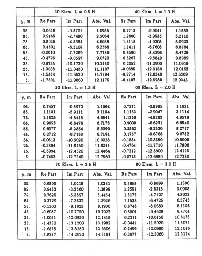
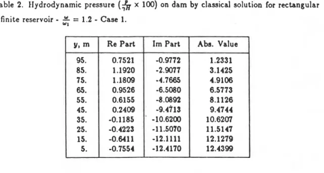
number of finite elements used to model infinite radiation is kept constant in all reservoir models and is equal to 10. Figure 1 shows a schematic view of these six models. Some results are presented for one excitation frequency w / w l = 1.2 in Table 1. Other results
are presented in Ref. 7. Results from the classical solution are listed in Table 2. The
BEM
results show that the difference in the absolute values is generally less than 5% w.r.t. available classical solutions. The model seems to represent the geometry quite faithfully. The transmitting boundary need not be located too far from the dam. Thus moving the transmitting boundary away, from 0.5 H to 1.0 H or farther, does not necessarily improve the results. All results are for a rigid reservoir foundation with a coefficient of reflectioncrR = 1.0 [3,7].
Case 2: Transmitting boundary is moved to an infinite regular section
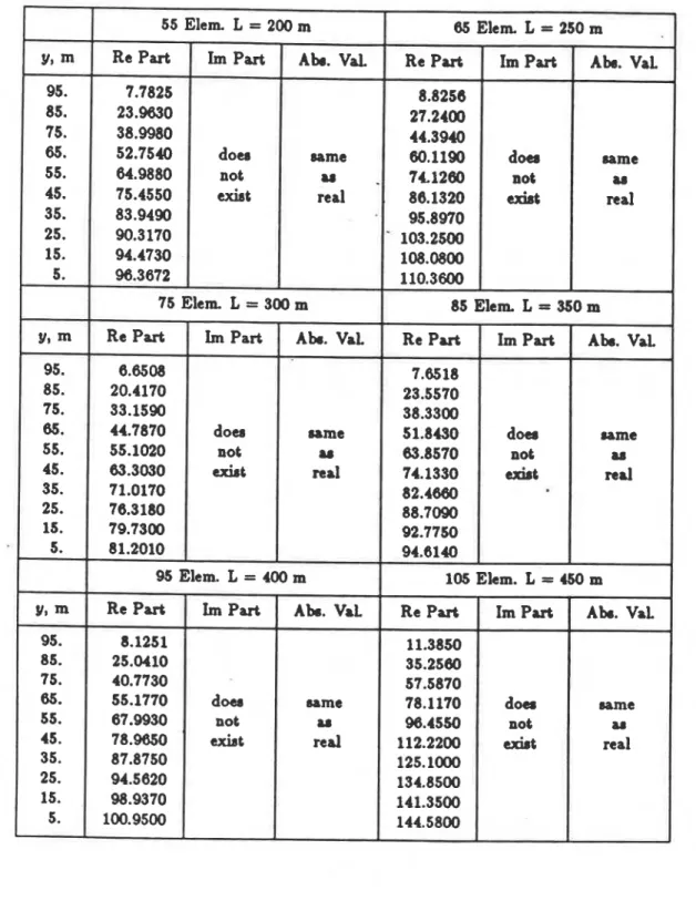
This part of the study has the objective of evaluating hydrodynamic pressures for one chosen shape of the reservoir with different locations of the transmitting boundary. However, the geometry of the irregular finite part is also changed. Five reservoir models are used. Their schematic view is presented in Fig. 2. The number of constant boundary elements changes from one model to another, but the number of finite elements at the
transmitting boundary remains the same. The results for one excitation frequency w/wl = 1.2 and a R = 1.0 are presented in Table 3. The results do not exhibit any particular trend
for this frequency and seem to depend only slightly on the location of the transmitting boundary in the rectangular infinite region of the reservoir. Further studies may be required to screen the behaviour for the representative frequency range.
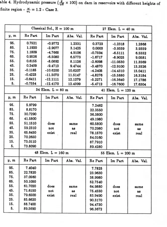
Case 3: Trapezoidal finite reservoir regjon is connected to an infinite regular region Five reservoirs with different lengths but with the same angles of the inclined bottoms have been studied. Thus, they have different heights of infinite section, while the actual dam height remains the same. The results are presented for one chosen excitation frequency w / w l = 1.2 and the rigid reservoir bottom with c u ~ = 1.0. Figure 3 shows a schematic view of the geometry of five models. Each model has a different number of constant boundary elements. The results are presented in Table 4. The results show an increase in the absolute values of hydrodynamic pressure with increase in length of the irregular finite portion of the reservoir. The results clearly depend on the overall geometry of the reservoir. The large increases in hydrodynamic pressures could be a function of specific parameters chosen and likely result from shifts in the true natural frequency of the considered reservoir with respect to w l , the natural frequency of the infinite rectangular reservoir.
Modelling of transmitting boundary
Earlier studies have shown that for an excitation frequency greater than w l the numer-
ical results of the analysis depend strongly on the modelling of the transmitting boundary
[7]. The results of these studies showed that even a fairly coarse division of the transmit- ting boundary did not introduce any appreciable error in hydrodynamic pressure values on the dam face, as long as the element size was not more than about 1/10 of the shortest wave length in the reservoir [7]. To obtain a direct measure of the effect of discretization used on the transmitting boundary (also called the far boundary), the first four eigen-
- values ( A ) together with respective eigenfrequencies (w) are calculated, for four different
one-dimensional meshes. The results obtained are presented in Table 5. Even with a 2-
element mesh, the difference between the first frequency obtained from a one-dimensional finite element solution and that obtained .from a continuum solution is remarkably small. The difference is very small when eight or more elements are used.
I
CONCLUSIONSThe following conclusions can be drawn:
1. The location of the transmitting boundary, which divides a reservoir into a finite part near a dam and the infinite rectangular part, can result in changes in the acting hydrodynamic forces when the geometry of the reservoir is changed.
2. If the irregular part is nearly rectangular the BEM results depend only slightly on the location of the transmitting boundary, while for a rectangular reservoir the results are virtually independent of the boundary location.
for modelling the transmitting boundary provided that their length is less than 1/10 of the shortest induced wave length in the reservoir.
ACKNOWLEDGEMENT
A part of this study derives from the author's Ph.D. research at Carleton University and was supervised by Professor J.L. Humar. The author thanks Dr. J.H. Rainer for his comments
.
REFERENCES
[I] Chopra, A.K., Chakrabarti, P., "Earthquake Analysis of Concrete Gravity Dams Including Dam-Water-Foundation Rock Interaction", Earthquake Engineering and Structural Dynamics, Vol. 9, 1981, pp. 303-383.
(21 Hall, J.F., Chopra, A.K., "Two Dimensional Dynamic Analysis of Concrete Gravity and Embankment Dams Including Hydrodynamic Effects", Vol. 10, 1982, pp. 305- 332.
[3] Hall, J.F., Chopra, A.K., "Dynamic Response of Embankment Concrete-Gravity and Arch Dams Including Hydrodynamic Interaction", Report No. UCBJEERC-89/39, Earthquake Engineering Research Center, University of California, Berkeley, Califor- nia, 1980.
[4] Hanna,
Y.G.,
Humar, J.L., "Boundary Element Analysis of Fluid Domain", Journal of Engineering Mechanics Division, ASCE, Vol. 108, 1982, pp. 436-450.[5] Liu, P.L.-F., Cheng, A.H.-D., "Boundary Solutions for Fluid-Structure Interactionn, Journal of Hydraulic Engineering, ASCE, Vol. 110, 1984, pp. 51-64.
161 Humar, J .L., Jablonski, A.M., "Boundary Element Reservoir Model for Seismic Anal- ysis of Gravity Dams", Earthquake Engineering and Structural Dynamics, Vol. 16,
1988, pp. 1129-1156.
[7] Jablonski, A.M., "Boundary Element Analysis of Earthquake Induced Hydrodynamic Pressures in a Water Reservoir", Ph.D. Thesis submitted to Carleton University, Ot- tawa, 1988.
[8] Moler, C.B., Stewart, G.W., "An Algorithm for Generalized Matrix Eigenvalues Prob- lems", SIAM Journal of Numerical Analysis, Vol. 10, 1973, pp. 241-265.
Table 1 . Hydrodynamic pressure ( x 100
)
on dam in rectangular infinite reservoirs with different location of the transmitting boundary-
'
= 1.2 ( 7 = unit weight of water andw1
H
= d n ~ n height)-
Case 1 . y, m 95. 85. 75. 65. 55. 45. 1 35. 25. 15. 5. y, m 95. 85. 75. 65. 55. 45. 35. 25. 15. 5. y, m 95. 85. 75. 65. 55. 45. 35. 25. 15. ' 5. 30 Elem. L = 0.5 H 40 Elem. L = 1.0 H 7 Re Part 0.6656 0.9465 0.8025 0.4501 -0.0010 -0.4776 -0.9255 -1.3038 -1.5854 -1.7801 Re Part 0.7713 1.2600 1.3115 1.1411 0.8560 0.5267 ' 0.2052 -0.06% -0.2714 -0.4107 Im Part -0.8701 -2.7480 -4.5384 -6.2 105 -7.7289 -9.0597 -10.1730 -11.0430 -11.6520 -11.9860 Ah. VaL 1.0955 2.9084 4.6088 6.2268.
7.7289 6.0723 - 10.2150 11.1197 11.7594 12.1175 Im Part -0.9041 -2.9535 -4.9205 -6.7608 -8.4296 -9.8849 -11.0900 -12.0150 -12.6340 -12.9280 50 Elem. L = 1.5 H Abr. VaL 1.1883 3.2110 5.0923 6.8564 8.4729 9.8989 11.0919 12.0152 12.6369 12.9345 60 Elem. L = 2.0 H Re Part 0.745'7 1.1181 1.1825 0.9653 0.6377 0.2712 -0.0813 -0.3804 -0.5994 -0.7483 A h . Val 1.1621 3.1114 4.9579 6.6840 8.2717 9.6782 10.8606 11.7808 12.41 10 12.7280 Im Part -0.8970 -2.9111 -4.8418 -6.6476 -8.2854 -9.7153 -10.9020 -11.8150 -12.4320 -12.7340 Re Part 0.7371 1.1153 1.1350 0.9000 0.5562 0.1757 -0.1884 -0.4764 -0.7212 -0.8728 Abr. Val. 1.1664 3.1184 4.W41 6.7179 8.3099 9.7191 10.9023 11.8241 12.4464 12.7560 r Im Part -0.8985 -2.9047 -4.8262 -6.6231 -8.2530 -9.6766 -10.8590 -11.7710 -12.3900 -12.6980 70 Elem. L = 2.5 H 80 Elem. L = 3.0 H Re P u t 0.6899 0.9433 0.7625 0.3729 -0.1100 -0.6087 -1.0651 -1.4350 -1.6875 -1.8277 Re Part 0.7658 1.2591 1.3172 1.1538 0.8748 0.5501 0.2311 -0.0441 -0.2499 -0.3977 Im Part -1.0218 -3.2560 -5.3897 -7.3832 -9.1923 -10.7750 -12.0950 -13.1200 -13.8280 -14.2020 Abr. Val. 1.0241 3.3899 5.4434 7.3926 9.1930 10.7922 12.1418 13.1982 13.9306 14.3191 - Im Part -0.8699 -2.8315 -4.7 127 -6.4725 -8.0683 -9.4608 -10.6150 -11.5020 -12.0990 -12.3060 Abr. VaL 1.1590 3.0988 4.8933 6.5745 8.1156 9.4768 10.6175 11.5021 12.1016 12.3124Table 2. Hydrodynamic pressure
(;k
x 100) on dam by classical solution for rectangularinfinite reservoir
-
$
= 1.2-
Case 1.Table 5. -Comparison of first four eigenfrequencies in 2D case for different finite element
meshes on the transmitting boundary.
Classical 1-d. FEM 1-d. FEM 1-d. FEM 1-d. FEM
Solution 2 Elem. 4 Elem. 8 Elem. 10 Elem
A? 0.000247 0.000260 0.000250 0.000247 0.000347 A; 0.002221 0.003169 0.002487 0.002286 0.002262 A; 0.006168 0.008207 0.006678 0.006492 A: 0.012090 0.017163 0.014081 0.013350 ~ 1 , s - I 22.62 23.20 22.77 22.66 22.64 wg, 3 - I 67.86 81.06 68.84 68.84 68.49 WJ, 3 - I 113.10
-
130.45 117.67 116.02 w,, 3 - I 158.34 188.65 170.87 170.87 166.38 L$
$
$Table 3. Hydrodynamic pressure ($ x 100) on dam in partially trapetoidal reservoirs in which the transmitting boundary is moved to an infinite region
-
+
=
1.2-
Case 2.55 Elem. L = 200 m 65 Elem L = 250 m
-
-
-y, m Re Part Im Part A h . Val Re Part Im Part Abe. Val.
95. 7.7825 8.8256
85. 23.9030 27.2400
75. 38.9980 44.3940
65. 52.7540 do- same 60.1190 doea name
55. 64.9880 not u
.
74.1260 not u45. I 75.4550 exbt real 86.1320 exbt real
35. 83.9490 95.8970 25. 90.3170
-
103.2500 15. 94.4730 108.0800 5. 96.3672 110.3600 75 Elem. L = 300 m 85 Elem. L = 350 m -y, m Re Part Im Part A h . VaL Re Part Im Part Abe. VaL
95. 6.6508 7.6518
85. 20.4170 23.5570
75. 33.1590 38.3300
65. 44.7870 do- same 51.8430 d a r aame
55. 55.1020 not u 63.8570 not u
45. 63.3030 urirt real 74.1330 exist red
35. 71.0170 82.4660
25. 76.3180 88.7090
15. 79.7300 92.7750
5. 81.2010 94.6140
95 Elem.
L
= 400 m 105 Ekm. L = 4!% my, m Re Part Im Part A h . VaL Re Part Im Part A h . Val.
95. 8.125 1 11.3850
85. 25.0410 35.2560
75. 40.7730 57.5870
65. 55.1770 doea same 78.1170 d a r name
55. 67.9930 not u 96.4550 not u
45. 78.9650 exist red 112.2200 udrt real
35. 87.8750 125.1OOO
25. 94.5620 134.8500
15. 98.9370 141.3500
Table 4. Hydrodynamic pressure ($ x 100) on dam in reservoirs with different heights of
infinite region
-
5
= 1.2-
Case 3.I
Claarical Sol.,H
= 100 m 27 Ekm. L = 40 my, m Re Part Im Part A h . Val. Re Put Im Part Atm. VaL
95. 0.7521 -0.9772 1.2331 0.3723 -1.2318 1.2868 85. 1.1920 -2.9077 3.1425 0.0005 -3.9359 3.9359 75. 1.1809 -4.7666 4.9106 -0.7594 -6.5111 6.5552 65. 0.9526 -6.5080 6.5773 -1.6717 -8.9025 9.0581 55. 0.6155 -8.0892 8.1126 -2.6098 -11.0530 11.3569 45. 0.2409 -9.4713 9.4744 -3.4870 -12.9100 13.3526 35. -0.1185 -10.6200 10.6207 -4.244 -14.4310 15.0411 25. -0.4223 -11.5070 11.5147 -4.8276 -15.5880 16.3184 15. -0.6411 -12.1111 12.1279 -5.2271 -16.3640 17.1786 5. -0.7554 -12.4170 12.4399 -6.4712 -16.7800 17.6304 34 Elem L = 80 m 41 E k m L = 120 m
y, m Re Part I m Part A h . Val. Re Part Im Part A h . VaL
95. 5.9799 7.2462
85. 8.8170 22.3550
75. 30.7290 36.3800
65. 41.5800 49.1980
55. 51.1510 doa =me 60.5800 does aame
45. 59.2310 not am 70.2980 not aa
35. 65.0450 exist real 78.1570 &t real
25. 70.2650 84.0160
15. 73.0110 87.7910
5. 73.8090 89.4280
48 Elem L = 160 m 55 Ekm. L = 200 m
y, m Re Part Im Part A b . Val. Re Part Im Part A b . VaL
95. 7.4040 7.7825
85. 22.7820 23.9630
75. 37.0580 38.9980
05. 50.1050 52.7540
55. 61.7020 does -me 64.9880 doen aame
45. 71.6150 not aa 75.4550 not a6
35. 79.6500 exist real 83.9490 exbt real
25. 85.6620 90.3170
15. 88.7400 94.4730
CASE I
W E ~ M E ~ M I 70EM
I RESERVOIR I I YCASE
2
INFINITE REGION I I m w M1
75ELEM Q5ELEM1
FlMTE REGION I 65ELEMI
85TRANSMITTNG BOUNDARY FOR
J- SOm -1- 50m -1- 50mL 50m _L 50m VARIOUS MODELS
T T T T T
CASE
3
LOCATION OF TRANSMlllllNG BOUNDARIES FOR VARIOUS MODELS
This paper is being distributed in reprint form by the Institute for Research in Construction. A list of building practice and research publications available from the Institute may be obtained by writing to Publications Section, Institute for Research in Construction, National Research Council of Canada, Ottawa, Ontario, KIA 0R6.
Ce document est distribub sous forme de tir6-A-part par
1'Institut de recherche en construction. On peut obtenir une liste des publications de l'lnstitut portant sur les techniques ou les recherches en matiere de Mtiment en krivant B la Section des publications, Institut de recherche en construction, Conseil national de recherches du Canada, Ottawa (Ontario), KIA 0R6.