Control of a compact, tetherless ROV for in-contact
inspection of complex underwater structures
The MIT Faculty has made this article openly available.
Please share
how this access benefits you. Your story matters.
Citation
Bhattacharyya, S., and H. H. Asada. "Control of a compact,
tetherless ROV for in-contact inspection of complex underwater
structures." The 2014 IEEE/RSJ International Conference on
Intelligent Robots and Systems, Chicago, IL, September 14-18, 2014.
As Published
https://ras.papercept.net/conferences/conferences/IROS14/
program/IROS14_ContentListWeb_3.html
Publisher
Institute of Electrical and Electronics Engineers (IEEE)
Version
Author's final manuscript
Citable link
http://hdl.handle.net/1721.1/90507
Terms of Use
Creative Commons Attribution-Noncommercial-Share Alike
Control of a Compact, Tetherless ROV for In-Contact Inspection of
Complex Underwater Structures
S Bhattacharyya
1and HH Asada
2Abstract— In this paper we present the dynamic modeling and control of EVIE (Ellipsoidal Vehicle for Inspection and Exploration), an underwater surface contact ROV (Remotely Operated Vehicle) for inspection and exploration. Underwater surface inspection is a challenging and hazardous task that demands sophisticated automation – as in boiling water nuclear reactors, water pipeline, submarine hull and oil pipelines inspection. EVIE is inspired by its predecessor, the Omni Submersible, in its ellipsoidal, streamlined, and appendage free shape. The objective for the robot is to carry inspection sensors – magnetic, acoustics or visual – to determine cracks on submerged surfaces. Unlike a robot moving in a practi-cally boundless fluid, contact forces complicate the dynamics by bringing in normal and frictional forces, both of which are highly non linear in nature. This makes the modeling much more challenging and the development of an integrated controller more difficult. In this paper we will discuss the preliminary design and hydrodynamic modeling of such a robot. We analyze in detail the controls for one of the many transitional states of this robot. Eventually all transitional states need to be integrated to develop a hybrid dynamical system which shall use a controller that can adapt to its different states.
IMPORTANT TERMS: NOMENCLATURE
X,Y,Z: World (inertial) coordinates [m]
f,q,y: Euler angles – roll, pitch and yaw angle. [radians] x,y,z: Body coordinates. [m]
u,v,w: surge, sway, heave; i.e., body centric velocities in x,y,z: [m/sec]
p,q,r: body centric roll, pitch and yaw rate. [radians/sec] a: angles of jet F3 and F4 from z in the xz plane [radians] b: angles for F1, F2, F5, F6 from the xy plane. [radians] g: angles of F1, F2, F5, F6 from x in the xy plane [radians] m: Vehicle mass. [kg]
Ixx,Iyy,Izz: Moment of inertia around x,y,z. [kg · m2]
X˙u,Y˙v,Z˙w:
Added mass associated with velocities u,v,w. [kg] K˙p,M˙q,N˙r:
Added moment associated with rotations p,q,r. [kg · m2]
Xu|u|,Yv|v|,Zw|w|:
Drag coefficient associated with velocities u,v,w. [kg/m] Kp|p|,Mq|q|,Nr|r|:
Drag moment associated with rotations p,q,r. [kg · m2]
Mu|u|: Coefficient for q torque caused by velocity u. [kg · sec2]
*Work has been partly supported by EPRI
1S Bhattacharyya is a PhD student in the Department of Mechanical Engineering, MITsampriti@mit.edu
2HH Asada is the Ford Professor of Engineering and Director of d’Arbeloff Laboratory for Information Systems and Technology, Department of Mechanical Engineering, MIT.asada@mit.edu
Cmm: Munk moment around y or z. [kg · sec2]
Uc: Free Stream velocity. [m/sec]
Fx,Fy,Fz: Net jet forces in x,y,z. [N]
Mx,My,Mz: Net torque in x,y,z. [N · m]
µk Coefficient of dynamic friction. [unitless]
N: Normal reaction force (when in contact). [N]
Fb: Buoyant Force. [N]
g: acceleration due to gravity. [m/sec2]
Su: effective mass (m X˙u)
Sv: effective mass (m Y˙v)
Sw: effective mass (m Z˙w)
Sp: effective moment of inertia (Ixx M˙q)
Sq: effective moment of inertia (Iyy N˙r)
Sr: effective moment of inertia (Izz N˙r)
I. INTRODUCTION
Inspection of underwater structures in constrained environ-ments is a challenging and hazardous task. Some examples are port security monitoring, inspection of nuclear reactor vessels, underwater cables, dams, ocean wrecks, and under-water oil pipelines [1], [2], [3]. These tasks demand different designs than unmanned underwater vehicles common in ocean engineering where operations are carried on mostly in an unbounded medium [4]. Present underwater inspection robots are tethered, bulky, and incapable of the smooth maneuvering necessary to access confined spaces . A small, tether-less, appendage free, highly maneuverable robot with multi degrees of freedom can swiftly reach and inspect areas a traditional tethered robot cannot [5]. This could prove invaluable to many applications including boiling water reac-tors (BWRs) inspection. Even quick inspections of submarine and ship hulls [6] can benefit from a small, swift robot.
A variety of underwater robots have been developed for such applications [7]; but there remains a need for advanced research to enable thorough inspection of underwater struc-tures for defects undetectable with mere visual inspection. We divide these inspection robots into two groups: non-contact, mostly for visual inspections; and non-contact, which perform more sophisticated surface inspection. The AIRIS 21 [3] is an example of a tethered underwater robot for contact crack inspection in reactors, while robotic fishes [8], [9] suited for non contact visual inspection have also been developed in industry and academia. Inspection robots with wheels (e.g. Surveyor) to operate underwater in nuclear facilities are also in use in the industry but are constrained to operate only on specific surfaces and are supported by cables [10]
At d’Arbeloff Lab, MIT, we developed an alternative solution: Omni Submersible, a 5 DOF, hydrodynamically unstable, highly maneuverable, ellipsoidal robot [11]. The robot was a tether-less, non contact, appendage free design for visual inspection in cluttered environments such as a BWR. Benefits of this design and the choice of the ellipsoid’s aspect ratio has been elaborated in [12]. However for internal cracks simple visual examination is insufficient. Volumet-ric inspection methods such as ultrasound or eddy current methods become indispensable [13]. The biggest challenge is these methods require contact. Therefore our goal is to extend the research to an underwater robot capable of moving while in contact with an underwater surface, as well as in free water. This largely changes the dynamics of the robot and requires a substantially different design.
Fig. 1. Omni Submersible (left) and EVIE(right)
EVIE is a contact-kind robot with a flat base. Figure 2 shows a conceptual design of a future version with a phased array sensor on its base for crack inspection, and an array of acoustic sensors for global localization to precisely locate defects . The task requires the electronics to be housed in the lower half of the robot with propulsion jets on top. Two prototypes have been made so far: EVIE-1 with jets aligned with the x,y,z axes; and EVIE-2 with jets angled for improved stability and control. The long term goal of this research is a tether-less inspection and exploration robot with navigation system capable of functioning in a complex underwater environment.
Initial tests of EVIE, presented here, focus on issues specific to contact with a surface. Although the design supports 5 DOF, here we consider only two: yaw and surge. We further limit our initial work to a horizontal surface where passive adjustment of normal force is possible by adjusting the weight of the robot. Finally, we neglect fluid movement on the assumption it is small compared to the robot’s velocity, as would generally be the case during a plant shutdown.
II. DESIGN CONCEPT
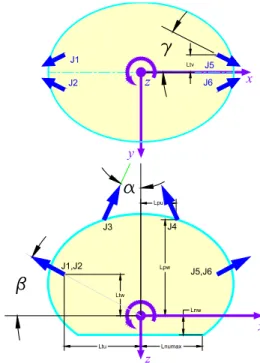
EVIE is an ellipsoidal robot, 203mm⇥152mm – an aspect ratio of 4:3,optimal for the system to be highly controllable [13]. Size can be adjusted to accommodate electronics and the sensors, though smaller size provides better maneuver-ability. The robot has 6 Jets, four ‘propulsion jets’ (J1, J2, J5, J6) and two ‘pressure jets’ (J3, J4); see figure 3. Propulsion
jets make an inward angle ofg in the xy plane which governs
Fig. 2. Picture (left) shows the kind of task EVIE is designed for. Red line shows a possible trajectory for weld seam inspection. Picture (right) shows the conceptual design of EVIE with a phased array sensor, camera for visual inspection and ultrasonic sensors on the body for global localization
the yaw-sway dynamics of the system. Non-zerog is needed
to ensure controllability of the system in the absence of friction [15]. For stability on a horizontal surface, which is our initial test case, we want the center of gravity (CG) of the robot to be below the center of buoyancy. This was attained by ballast at the bottom of the robot.For more complex cases (e.g. inspecting a vertical wall, or going around a pipe) we would need to adjust the CG location. Note jets J1, J2, J5
and J6 are at an angle b such that they pass through the
CG of the system. This eliminates thrust induced pitching. However friction or surface curvature might demand active pitch control. This is attained by orienting the two pressure
jets J3 and J4 at an angle ofa as shown in figure 3.
Fig. 3. Top and Side View of EVIE-2. Arrows indicate the force direction
III. VEHICLE MODELING
A. Forces Acting on the Robot in Contact with the Surface An underwater robot moving in contact with a surface has many interesting phenomena involved in its dynamic modeling. We broadly divide the forces acting on the robot
into thrust, contact, hydrodynamic, and body forces. Thrust is caused by the propulsion and pressure jets. The contact forces are friction and normal forces. Hydrodynamic forces and moments include drag, Munk moment, ground effect, and lift [14], [15]. Body forces include weight and inertial forces. These forces introduce complexities of varying de-gree, and some (friction in particular) cannot be assumed known a priori. We discuss how these contribute to the equations of motion of this robot and consider which terms are most critical. Ultimately the goal is to synthesize a controller using a simplified design model with sufficient robustness to contend with dynamics and other effects not fully captured in the design model.
Thrust Forces: Thrust forces are produced by the
sub-mersible micro pumps housed inside the robot. For small g
the velocity u is dominant over velocity v. Pressure jets are J3 and J4 provide additional torque to prevent pitch; these can be supplemented by jets in the lower half to enable full pitch control for the robot.
The forces and moments along the body axes due to the Jets 1-6 can be given as :
Jet forces
Fx= (F4 F3)sina + (F1 F5 + F2 F6)cosg cosb
Fy= (F1 + F5 F2 F6)sing cosb Fz= (F3 + F4)cosa + (F1 + F2 + F5 + F6)sinb (1) Jet Moments Mx=(F1 + F5 F2 F6)sinbLtv+ (F1 + F5 F2 F6)sing cosbLtw My=(F3 F4)cosaLpu +(F3 F4)sinaLpw +(F1 + F2 F5 F6)sinbLtu +(F1 + F2 F5 F6)cosb cosgLtw Mz=( F1 F6 + F2 + F5)cosg cosbLtv+ ( F1 F6 + F2 + F5)sing cosbLtu (2)
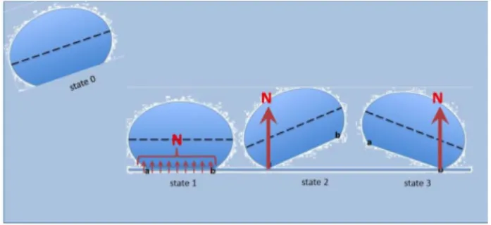
Contact Forces: Contact forces introduce a discrete change in vehicle dynamics as it transitions between the status shown in figure 4: free floating (state 0), contacting across surface (our desired condition) (state 1), and point contact when pitching nose up or nose down (state 2 and state 3). We develop generalized equations that are valid for all cases: setting the normal force, N = 0 is equivalent to placing the robot in a boundless fluid. On the surface, the normal force is not constant. In state 1 (flat), the magnitude and location of the normal force varies with velocity; in states 2 and 3 the normal force also varies with pitch angle (due to hydrodynamic lift) as well as pitch rate (since the CG moves as pitch changes).
The other possible states of the robot are roll, and roll and pitch combined. Neither roll nor pitch is beneficial during inspection. But the pitching moment is 10x larger than the roll moment because |v| << |u|. Furthermore, we intend a future prototype will have pitch control to climb over
Fig. 4. Transitional states of the Robot. Location of the normal for, N, varies with pitch. State 0 is in the boundless fluid whereas states 1, 2 and 3 are on an horizontal inspection surface.
obstacles. Therefore, in this paper we include pitch, but not roll. The flat bottom of the robot is sufficient to counteract small roll forces.
Friction is the other contact force that is highly non linear and coupled with the normal force. Friction models in a hydrodynamic environment can be quite complex. At the low speeds required for inspection, transition between static and dynamic friction, like Strikebeck effect [16], need to be considered. Depending upon the velocity of the robot and surface roughness, a thin layer of fluid between the contacting surfaces can cause viscous friction. Our robot has weight minus buoyancy of approximately 0.1N; taking the coefficient of friction as 10% friction force is on the order of 0.01N compared to jet forces of order 0.1N. Friction is large enough to merit inclusion, but not so large as to warrant detailed analysis. We assume the moving robot
has a kinematic friction force of µkN. For the research
discussed here static friction is not used: we will work with a moving robot. Note, however, friction coefficient may approach 100% on rusty or concrete surfaces. The control system must be able to handle such cases without a priori knowledge of the surface.
Hydrodynamic Forces: The main hydrodynamic forces and moments that can influence the robot are the drag, Munk moment, and lift, each of which may depend on ground effects [17]. Hydrodynamic drag is quadratic for high Reynolds number, as in our case; we therefore neglect
linear drag terms of the form Xuu. Our calculations indicate
the lift term is a small correction to the effective weight of the robot; as motion in z is not our focus, we do not include a separate lift term. The term Xu|u|, Yv|v| and Zw|w| are hydrodynamic coefficients that account for the different lateral and longitudinal forces acting on the body. The dominant velocity of the robot is along u; hydrodynamic moments associated with motion in u are accounted for by
Mu|u|. The Munk Moment is a destabilizing moment. In the
absence of pitch, the Munk moment is exclusively in the xy plane and is given by
where z is the sideslip angle. In our case, with zero pitch and still water, u = U cosz and v = U sinz so
Mm= (Y˙v X˙v)(U sinz)(U cosz)
=Cmmuv (4)
where Cmm= (Y˙v X˙v). [14]
Therefore, Munk moment enters both the pitch and the yaw equations of motions.
The hydrodynamic coefficients are constant for a body in an unbounded fluid. However near a surface the values depend upon the distance to the ground and the angle of attack, and are more complicated to calculate. Ground effect can be defined as the change of the flow field due to the presence of ground. In this paper we only deal with a perfect contact case, that is the contribution of the fluid layer between the flat bottom and the inspection surface has not been analyzed. It is to be noted ongoing work is incorporating the effects due to this fluid layer, which in turn changes the magnitude of the above mentioned hydrodynamic forces. In such a case, analytical formulation of the actual phenomenon is hard and standard fluid dynamics software are used to compute the hydrodynamic coefficients.
Below are given the generalized equations of motions for our non linear model of the robot.
B. Simplified Equation of Motions, neglecting Roll
Note the equation for ˙p is derived from the requirement ˙f = 0.
˙u = 1
(m X˙u)(Fx (mg Fb)sinq + Nsinq
Xu|u|u|u| µkNVu m(qw rv)) ˙v = 1 (m Y˙v)(Fy Yv|v|v|v| µkN v V mru) ˙w = 1 (m Z˙w)(Fz+ (mg Fb N)cosq Zw|w|w|w| µkNw V +mqu)
˙p = sec2q(qsinf + r cosf) ˙q tanq( ˙qsinf + ˙rcosf)
˙q = 1
(Iyy M˙q)(My µkN
u VLnw
+NLnwsinq FbLbsinq Mq|q|q|q| + Mu|u|u|u| +Cmmuw)
˙r = 1
(Izz N˙r)(Mz Nr|r|r|r| +Cmmuv)
˙q =q ˙ y =cosqr
˙X =ucosq +v( siny)+w(cosq siny sinq cosy siny) ˙Y =ucosq siny +vcosq cosy siny)
+w(cosq siny sinq cosy siny) ˙Z =wcosq
In state 1 – contact with a surface, without pitch or roll, –
we have Z =f = q = 0 and the remaining equations simplify
further.
˙u = 1
(m X˙u)(Fx Xu|u|u|u| µkN
u V +mrv) ˙v = 1 (m Y˙v)(Fy Yv|v|v|v| µkN v V mru) ˙r = 1 (Izz N˙r)(Mz Nr|r|r|r| +Cmmuv) ˙ y =r ˙X =ucosy vsiny ˙Y =usiny +vcosy
(5)
For quantitative analysis we calculate the hydrodynamic coefficients using published formulas for ellipsoids. These formulas measure moments around the geometric center, whereas we wish to do so around an off-center CG. In particular, Mu|u| is zero if the CG is at the geometric center, but would not be so for us. We approximate the torque from the drag force in x, Xu|u|u|u|, times the distance from the CG to the geometric center, Lcgw. We varied Mu|u| as Xu|u|Lcgw
to 2Xu|u|Lcgw in our simulations, and for the desirable (non
pitched case) it doesn’t make any significant difference.
IV. LINEARIZEDMODEL
In our research we break the study of the robot into three discrete states as shown in figure 4. State 1 is the desired state: the robot should move on a horizontal inspection surface making reliable contact with it at all times. State 2 and 3 are the undesirable states that the robot can enter into, due to different non ideal situations. These states cause detachment of the sensor from the surface and interrupt inspection. Our goal is to find the necessary conditions to be satisfied to remain in the desirable state, and then incorporate stability and control on that inspection surface. In other words, we need to find the conditions that cause such undesirable pitching and ensure they do not happen. Note, state 0 will not be discussed as that was already demonstrated by the Omni Submersible.
The robot will pitch nose up if the net torque around the CG is positive, and nose down if the net torque is negative. The net torque includes contribution from the normal force. N. The effective location of the normal force varies, but at the moment of pitching nose up it will be at point ’a’ of figure 4 resulting in a negative torque; whereas at the moment of pitching nose down it will be at point ’b’ giving a positive
torque. Depending on angles b and g, jets J1 and J2 may
pass above or below the CG, creating a negative or positive torque. In addition, the z component of the jet forces adds to N.
To estimate a stability condition we assume constant u so the jet forces exactly balance drag and friction forces; we also take v = 0 i.e. no yaw or lateral motion. To be stable against nose-down pitch u must remain below
unopitch<
v u u
t (mg Fb)Lnumax
Xu|u|⇣Ltbw (Ltbu+Lnumax)tanbcosg
⌘
where for simplicity we have left out the friction force. Similarly for nose-up
unopitch<
v u u
t (mg Fb)Lnumax
Mu|u| Xu|u|⇣Ltbw (Ltbu Lnumax)tanbcosg
⌘ (7) Neither equation 6 nor 7 have a real solution (i.e., the robot has no pitch for any velocity u) if
Ltbw MXu|u|u|u|
Ltbu+Lnumaxcosg < tanb <
Ltbw MXu|u|u|u|
Ltbu Lnumaxcosg (8)
in which case – neglecting friction – the robot is stable against pitch.
Equation 8 establishes EVIE can be stable against pitch at high speed, where hydrodynamic forces dominate and we neglect friction. Next we establish conditions under which the robot is stable at low speed, where hydrodynamic forces are negligible and we consider only friction. We find
µk<LLnumax
tw+Lnw (9)
for a chosenb.
For EVIE, the condition in equation 8 can be met by
setting g and b such that the jet forces pass through the
CG. However, if the condition of equation 9 is not met, pitching may occur at low speed due to friction. This is corrected using J3 and J4. The controller monitors an onboard accelerometer to detect pitch, and uses J3 or J4 to bring the robot back to it’s desired state.
Assuming we satisfy the above condition, we next lin-earize this non linear model about an equilibrium point, or trim condition. The definition of linearization implies finding a situation for which ˙x = f (x,u) = 0 where x represents your state variables. Linearization is justified since the system dy-namics doesn’t change drastically in the region of operation. Assuming we satisfy the constraints discussed, here the robot is taken to be moving only in the XY plane: the robot has
no velocity in z and no pitch or roll. Therefore w, p, q, q,
f are all zero. We look at the states u,v,r,y.
Let us assume for our trim state the robot is on the surface
and is moving with a velocity Uc = .15m/sec in the x
direction and no yaw or y velocity (v = r =y = 0). The
input forces F1, F2, F5 and F6 which to meet the trim state condition ˙x = f (x,u) = 0 are F1=F2=0.2N. The normal force in this case is a constant, and can be expressed as follows:
N = mg Fb+Fzcosq Fxsinq (10)
This is valid only for a constant pitch angle.
We would like to control the heading angle, as well as the speed. Hence we choose the 4 state variables, u,v,r,y. The generalized linearized state space model is given by
2 6 6 4 D ˙u D ˙v D˙r D ˙y 3 7 7 5 = 2 6 6 6 4 2Xu|u|Uc Su 0 0 0 0 µkN SvUc mUc Sv 0 0 CmmUc Sr 0 0 0 0 1 0 3 7 7 7 5 2 6 6 4 Du Dv Dr Dy 3 7 7 5 + 2 6 6 4 1 Su 0 0 0 1 Sv 0 0 0 1 Sr 0 0 0 3 7 7 5 2 4FFxy Mz 3 5 (11) V. CONTROL DESIGN
The system is modeled considering predominant motion in surge.This open loop plant is inherently unstable due to the associated Munk moment which depends on the difference of the added mass in x and y. For longitudinal motion of such a spheroidal system, the sway yaw dynamics give rise to a positive eigen value that contribute to the instability of the system [6]. This is simulated in figure 5.
Fig. 5. Munk Moment simulation using the non linear model
To have a good control authority on a robot requires a good design. For example, the open loop behavior of the
robot withb = 0 and g = 0 in EVIE-1 gave rise to a yawing
moment at a constant pitch angle (as we will see in figure 10). This was investigated through our simulations and we were
able to reproduce the effect. The reason is due tob = 0 the
robot had considerable moment arm along z, causing a nose down pitch. Further, the Munk moment caused the circular motion as seen in figure 6 at a constant but small pitch angle. Hence the robot never moved forward but stayed stuck in a place.
The open loop poles of the system are shown in figure 7.
As Fyµ sing, if g = 0 it can be seen, there is no control
over v: the model is uncontrollable if friction coefficient is 0
(in a boundless fluid). Larger g would render more control
over v and yaw, but it compromises the thrust force in u. As
the desired velocity is primarily u, we chose as our g = 30
which gives a considerable control authority on yaw without greatly penalizing the thrust force in ’u’ .
Fig. 7. Open loop poles
Once we assume that the robot is now only operating on the 2D horizontal inspection plane (by satisfying the constrains mentioned before), we can stabilize it by mitigat-ing against undesirable yawmitigat-ing moments usmitigat-ing LQR or PID controller. Note the control system for the full hybrid model would involve a much more complex control algorithm-which can take into account the switching between the different states. Different sophisticated AUV and underwater glider algorithms are prevalent [18]. In our future research integrating the control algorithms for different states will be indeed mandatory.
For the simulation, we assume the robot has independent control over all the jets and has a full state feedback system.
A LQR controller is designed. As shown before, Fy or Fx
or Mz are combinations of various jets. We map back to the
combination to get individual jet forces.
Since b is small, Fy is limited; therefore we penalize
this input by putting a corresponding large weight in the R matrix. For our prototype, the maximum jet force in y is 0.1N, i.e.
Fy= (F1 + F5 F2 F6)sing cosb < 0.1 (12)
Below is a example of the control weighting matrix R, and the state weighting matrix Q that can be used in our prototype.
diag ⇥1 143 0.0001⇤ (13)
diag ⇥1 700 1 100⇤ (14)
A optical sensor for underwater localization on the target surface is under development, details of which are being published in a complementary paper. This sensor will be allowing the the robot to precisely locate itself, and give us
both the coordinates and the velocity of the robot at the area of inspection. Keeping that in mind, developing a full state feedback was therefore necessary.
Fig. 8. Closed loop control using LQR on linear model. Figure (a) shows the linear model control. Figure (b) shows the use of the controller on the non linear model
For our current prototype which has only a yaw angle feedback, a PD controller is designed, like in the Omni Submersible [19], which corrects for the instability due to the Munk Moment. This can be represented as:
DMz = K1d
dt(yd(t) y(t)) + K2(yd(t) y(t)) (15)
whereydis the desired yaw or heading angle, and K1and
K2 are derivative and proportional gains.
VI. HARDWAREIMPLEMENTATION ANDEXPERIMENTAL
RESULTS
A. Design
Two prototypes of EVIE have been developed so far. EVIE-1 was a simple demonstration of a surface contact un-derwater robot. It had two pressure jets and four propulsion jets. None of the jets were angled. This system did not have any control authority in ’y’ and poor yaw control unless the outlets were far apart from each other.
Fig. 9. EVIE-1. 4 pumps in the submersible part. Straight jets. Water sealed part contains electronics including IMU and localization sensors
We performed experiments on EVIE-1 by making it slightly heavier than neutral buoyancy and putting it on the
horizontal surface under water. When jets J1 and J2 were turned on to propel the robot in u, the robot instead of going forward suffered a nose down pitch and went in circles as seen in the simulation in figure 6. In figure 10 one sees the
small q angle of the robot as it yaws.
EVIE-1 had jets that come out straight and therefore the length of moment arm in w to the center of gravity gave rise to a pitch down moment. The frictional force also contributed to the pitch down moment. The velocity u being small, the drag couldn’t compensate for this. The Munk moment, combined with accidental sideslip perturbation, resulted in a constant yaw rate and the robot going in the circles as shown in figure 10.
Fig. 10. Nose down pitching moment exhibited by prototype 1 of EVIE
EVIE-2 has two kinds of jets: propulsion and pressure. As explained in the design concepts, to counter thrust induced
pitching the angle b was introduced to reduce the moment
arm to the CG. For simplicityb is chosen such that the force
vector pass through the estimated center of gravity thereby minimizing the pitch otherwise caused by placing the jets in the upper half of the robot.
Fig. 11. EVIE-2 with angled jets. Note the line of force of the thrust jets pass through the estimated CG
EVIE-2 doesn’t pitch when jet1 and 2 are turned on. However, it yaws due to Munk moment. Since in hardware, full state feedback is not fully developed yet, we use a PD controller and check on the closed loop response. Figure 12 shows the open and closed loop response, with the robot moving straight on contact with a low friction surface (µk<
.3). B. Results
To test the validity of the controller, a disturbance was injected to the system by forcing jet 2 to remain off for
50msec. As shown in figure 12 the controller was success-fully able to stabilize it. Data is from the on-board IMU with an integrated Kalman filter to remove noise.
Fig. 12. Closed Loop Control of EVIE-2. Comparing to open loop (left). Recovery from disturbance (right). Angles measured by on-board IMU.
Finally, figure 13 shows the comparison of the closed loop and open loop trajectory. As seen, for the given friction, a simple PD controller is able to control the heading angle successfully. For very high friction, one should note the Munk moment would face a breaking torque that would substantially reduce the yaw rate. Experiments with different friction models are yet to be performed.
0.15 0.2 0.25 0.3 0.35 −0.18 −0.16 −0.14 −0.12 −0.1 −0.08 −0.06 −0.04 −0.02 0 x (m) y (m)
XY Trajectotory: Experimental Data
OL CL
Fig. 13. Experimental data on open(blue) and closed(red) loop trajectory
VII. CONCLUSION
We have designed a novel underwater robot for surface inspection. The robot slides with its shell in contact with the surface allowing for a variety of inspection tools (opti-cal, magnetic, acoustic). The body has no appendages and communication is wireless, making it ideal for confined spaces. The appendage-free design is hydrodynamically un-stable and relies on a control system to achieve stability. Detailed modeling and analysis has been presented based on simulation with a full, non-linear model. Control techniques for stabilization have been discussed for the linearized model operating on a 2D horizontal surface. Initial experimental results for yaw stabilization on an horizontal surface has also been shown. To simplify our experiments with contact forces, EVIE as presented here has a low CG; to operate on anything other than a horizontal surface, it must run the
pressure pumps continuously and at higher power. Future versions of EVIE will shift the CG, perhaps dynamically, to minimize the power consumed by pressure pumps. The unique geometry of EVIE creates new opportunities to use surface effects as an integral part of the control system. We explored contact forces in this paper, both predictable normal force and unpredictable friction force. Subsequent work will incorporate ground effects and its role in the stability and control of the system. A more complete state feedback controller is also under development. Hydrodynamic effects and variable friction forces are complex and difficult to model very precisely; however, the combination of controller, sensors, and propulsion should provide robustness against unmodeled dynamics. The goal in subsequent work is to incorporate additional states of the robot and develop an integrated controller for the system.
REFERENCES
[1] J.A. Ramirez, R. Vasquez, L. Gutierrez, D. Florez, Mechanical/Naval Design of an Underwater Remotely Operated Vehicle (ROV) for Surveillance and Inspection of Port Facilities, Proc. of the 2007 ASME International Mechanical Engineering Congress and Exposition, 2007. [2] K. Asakawa, J. Kojima, Y. Ito, S. Takagi, Y. Shirasaki, N. Kato, ”Autonomous Underwater Vehicle AQUA EXPLORER 1000 for In-spection of Underwater Cables”, Proc. of the 1996 IEEE Symposium on Autonomous Underwater Vehicle Technology, 1996, pp 10-17. [3] K. Koji, Underwater inspection robot -AIRIS 21, Nuclear
Engineer-ing and Design, Vol., 188, 1999, 367-371.
[4] Hanumant Singh,Roy Armstrong,Gilbes, Fernando and Ryan Eustice and Chris Roman,and Oscar Pizarro, and Juan Torres, ” Imaging Coral I: Imaging Coral Habitats with the SeaBED AUV”, Subsurface Sensing Technologies and Applications, vol., no., pp. 5,1, 25-42, 2004 [5] A. Mazumdar, M. Lozano, A. Fittery and H.H Asada, A compact,
maneuverable, underwater robot for direct inspection of nuclear power piping systems, Robotics and Automation (ICRA), 2012 IEEE Inter-national Conference on , vol., no., pp.2818,2823, 14-18 May 2012 [6] J. Vaganay, M. Elkins; D. Esposito.; O’Halloran; F Hover,; M Kokko,
”Ship Hull Inspection with the HAUV: US Navy and NATO Demon-strations Results,” OCEANS 2006 , vol., no., pp.1,6, 18-21 Sept. 2006 [7] Junku Yuh, .”Design and control of autonomous underwater robots: A
survey”, Autonomous Robots 2000 , vol., no., pp.8,1, 7-24 [8] P Valdivia y Alvarado, K. Youcef-Toumi., Performance of Machines
with Flexible Bodies Designed for Biomimetic Locomotion in Liquid Environments, Robotics and Automation, 2005. ICRA 2005. Pro-ceedings of the 2005 IEEE International Conference on , vol., no., pp.3324,3329, 18-22 April 2005
[9] Tan Xiaobo, D Kim, N Usher, D Laboy, J Jackson, A. Kapetanovic, J. Rapai; B Sabadus, Xin Zhou, ”An Autonomous Robotic Fish for Mobile Sensing,” Intelligent Robots and Systems, 2006 IEEE/RSJ International Conference on , vol., no., pp.5424,5429, 9-15 Oct. 2006 [10] A. Rohrabacher; R. Carlton; F Gelhaus , Considerations in the de-velopment and implementation of a robot for nuclear power facilities, Transactions of the American Nuclear Society, v.54, p.186; September 1987
[11] A . Mazumdar, M. Lozano, HH Asada, Omni Egg: A smooth spheroidal appendage free robot capable of 5 DOF motion, Oceans 2012, pp.1-5, IEEE 2012
[12] A . Mazumdar, HH Asada, Control Configured Design of Spheroidal, Appendage Free, Underwater Robot, IEEE Transactions on Robotics, vol., no., pp. 30, 2, 448-460, April 2014.
[13] F. Dirauf, B. Gohlke, and E. Fischer, Innovative Robotics and Ultrason-ice Technology at the Examination of Reactor Pressure Vessels in BWR and PWR Nuclear Reactor Power Stations, Insight-Non-Destructive Testing and Condition Monitoring, vol. 42(9), 2000, pp. 590-593
[14] M. Triantafyllou, F. Hover, Maneuvering and Control of Marine Vehicles, MIT Course Notes, Department of Ocean Engineering, MIT, 2003, MIT.
[15] J.N. Newman, Marine Hydrodynamics, MIT Press, Cambridge Mas-sachusetts, 1977
[16] Wong, H; Chieh and Umehara, Noritsugu and Kato, Koji, Fric-tional characteristics of ceramics under water-lubricated condi-tions,Tribology Letters,November 1998, ISBN:1023-8883
[17] Erin Blevins and George V Lauder,Swimming near the substrate: a simple robotic model of stingray locomotion, 2013 Bioinspir. Biomim. 8 016005
[18] N. E Leonard and J.G Graver, Model Based feedback control of autonomous underwater gliders, IEEE J. Oceanic Eng.,vol., no., pp., 26,4, 633-645, 2001.
[19] A. Mazumdar, A. Fittery, M. Lozano, H. Asada, Active Yaw Stabiliza-tion for Smooth Highly Maneuverable Underwater Vehicles, Proceed-ings of the 2012 ASME Dynamic Systems and Controls Conference.