HAL Id: hal-00296345
https://hal.archives-ouvertes.fr/hal-00296345
Submitted on 4 Oct 2007
HAL is a multi-disciplinary open access
archive for the deposit and dissemination of
sci-entific research documents, whether they are
pub-lished or not. The documents may come from
teaching and research institutions in France or
abroad, or from public or private research centers.
L’archive ouverte pluridisciplinaire HAL, est
destinée au dépôt et à la diffusion de documents
scientifiques de niveau recherche, publiés ou non,
émanant des établissements d’enseignement et de
recherche français ou étrangers, des laboratoires
publics ou privés.
ships on aerosols, clouds, and the radiation budget
A. Lauer, V. Eyring, J. Hendricks, P. Jöckel, U. Lohmann
To cite this version:
A. Lauer, V. Eyring, J. Hendricks, P. Jöckel, U. Lohmann. Global model simulations of the impact of
ocean-going ships on aerosols, clouds, and the radiation budget. Atmospheric Chemistry and Physics,
European Geosciences Union, 2007, 7 (19), pp.5061-5079. �hal-00296345�
www.atmos-chem-phys.net/7/5061/2007/ © Author(s) 2007. This work is licensed under a Creative Commons License.
Chemistry
and Physics
Global model simulations of the impact of ocean-going ships on
aerosols, clouds, and the radiation budget
A. Lauer1, V. Eyring1, J. Hendricks1, P. J¨ockel2, and U. Lohmann3
1DLR-Institut f¨ur Physik der Atmosph¨are, Oberpfaffenhofen, Germany
2Max Planck Institute for Chemistry, Mainz, Germany
3Institute of Atmospheric and Climate Science, Zurich, Switzerland
Received: 11 June 2007 – Published in Atmos. Chem. Phys. Discuss.: 2 July 2007
Revised: 10 September 2007 – Accepted: 21 September 2007 – Published: 4 October 2007
Abstract. International shipping contributes significantly to the fuel consumption of all transport related activities.
Spe-cific emissions of pollutants such as sulfur dioxide (SO2)
per kg of fuel emitted are higher than for road transport or aviation. Besides gaseous pollutants, ships also emit var-ious types of particulate matter. The aerosol impacts the Earth’s radiation budget directly by scattering and absorbing the solar and thermal radiation and indirectly by changing cloud properties. Here we use ECHAM5/MESSy1-MADE, a global climate model with detailed aerosol and cloud mi-crophysics to study the climate impacts of international ship-ping. The simulations show that emissions from ships sig-nificantly increase the cloud droplet number concentration of low marine water clouds by up to 5% to 30% depending on the ship emission inventory and the geographic region. Whereas the cloud liquid water content remains nearly un-changed in these simulations, effective radii of cloud droplets decrease, leading to cloud optical thickness increase of up to 5–10%. The sensitivity of the results is estimated by us-ing three different emission inventories for present-day ditions. The sensitivity analysis reveals that shipping con-tributes to 2.3% to 3.6% of the total sulfate burden and 0.4% to 1.4% to the total black carbon burden in the year 2000 on the global mean. In addition to changes in aerosol chemi-cal composition, shipping increases the aerosol number con-centration, e.g. up to 25% in the size range of the accumu-lation mode (typically >0.1 µm) over the Atlantic. The to-tal aerosol optical thickness over the Indian Ocean, the Gulf of Mexico and the Northeastern Pacific increases by up to 8–10% depending on the emission inventory. Changes in aerosol optical thickness caused by shipping induced modifi-cation of aerosol particle number concentration and chemical composition lead to a change in the shortwave radiation bud-get at the top of the atmosphere (ToA) under clear-sky
condi-Correspondence to: A. Lauer
(axel.lauer@dlr.de)
tion of about −0.014 W/m2to −0.038 W/m2for a global
an-nual average. The corresponding all-sky direct aerosol
forc-ing ranges between −0.011 W/m2 and −0.013 W/m2. The
indirect aerosol effect of ships on climate is found to be far larger than previously estimated. An indirect radiative effect
of −0.19 W/m2to −0.60 W/m2(a change in the atmospheric
shortwave radiative flux at ToA) is calculated here, contribut-ing 17% to 39% of the total indirect effect of anthropogenic aerosols. This contribution is high because ship emissions are released in regions with frequent low marine clouds in an otherwise clean environment. In addition, the potential impact of particulate matter on the radiation budget is larger over the dark ocean surface than over polluted regions over land.
1 Introduction
Besides gaseous pollutants such as nitrogen oxides
(NOx=NO+NO2), carbon monoxide (CO) or sulfur dioxide
(SO2), ships also emit various types of particulate matter
(Eyring et al., 2005a). Due to low restrictive regulations for international shipping and the use of low quality fuel by most ocean-going ships, shipping contributes for example to
around 8% to the present total anthropogenic SO2emissions
(Olivier et al., 2005). The aerosol impacts the Earth’s radi-ation budget directly by scattering and absorbing solar and thermal radiation and indirectly by changing cloud proper-ties. Aerosols emitted by ships can be an additional source of cloud condensation nuclei (CCN) and thus possibly re-sult in a higher cloud droplet concentration (Twomey et al., 1968). The increase in cloud droplet number concentration can lead to an increased cloud reflectivity. Measurements in the Monterey Ship Track Experiment confirmed this hypoth-esis (Durkee et al., 2000; Hobbs et al., 2000). This mech-anism can also cause anomalous cloud lines, so-called ship tracks, which have often been observed in satellite data (e.g.
Conover, 1966; Nakajima and Nakajima, 1995; Schreier et al., 2006). In addition, aerosols from shipping might also change cloud cover and precipitation formation efficiency as well as the average cloud lifetime.
Although a rapid growth of the world sea trade and hence increased emissions from international shipping are expected in the future (Eyring et al., 2005b), the potential global influ-ence of aerosols from shipping on atmosphere and climate has received little attention so far. Available studies on the global impact of ship emissions on climate concentrate on
greenhouse gases such as carbon dioxide (CO2), methane
(CH4)or ozone (O3)as well as the direct effect of sulfate
particles (e.g. Lawrence and Crutzen, 1999; Endresen et al., 2003; Eyring et al., 2007). Concerning the indirect aerosol effect by ship emissions, only rough estimates for sulfate plus organic material particles from global model simula-tions without detailed aerosol and cloud physics (Capaldo et al., 1999) are currently available. The overall indirect ef-fect due to international shipping taking into account aerosol nitrate, black carbon, particulate organic matter and aerosol liquid water in addition to sulfate as well as detailed aerosol physics and aerosol-cloud interaction has not been assessed in a fully consistent manner yet.
The emissions of gaseous and particulate pollutants scale with the fuel consumption of the fleet. Ideally, the fuel con-sumption of the world-merchant ships calculated from en-ergy statistics (Endresen et al., 2003; Dentener et al., 2006) and based on fleet activity (Corbett and K¨ohler, 2003; Eyring et al., 2005a) should be the same, but there are large dif-ferences between the two approaches and there is an ongo-ing discussion on its correct present-day value (Corbett and K¨ohler, 2004; Endresen et al., 2004; Eyring et al., 2005a). In addition, various vessel traffic densities have been
pub-lished over the last years. In order to address these
un-certainties, we apply three different emission inventories for shipping (Eyring et al., 2005a; Dentener et al., 2006,
Wang et al., 20071). We use the global aerosol climate
model ECHAM5/MESSy1-MADE, hereafter referred to as E5/M1-MADE, that includes detailed aerosol and cloud mi-crophysics to study the direct and indirect aerosol effects caused by international shipping. The model and model sim-ulations are described in Sect. 2. To evaluate the performance of E5/M1-MADE we have repeated the extensive intercom-parison of the previous model version ECHAM4/MADE with observations (Lauer et al., 2005). The comparison to observations shown here focuses on marine regions and is summarized in Sect. 3. Section 4 presents the model results and Sect. 5 closes with a summary and conclusions.
1Wang, C., Corbett, J. J., and Firestone, J.: Improving Spatial Representation of Global Ship Emissions Inventories, Environ. Sci. Technol., under review, 2007.
2 Model and model simulations
2.1 ECHAM5/MESSy1-MADE (E5/M1-MADE)
We used the ECHAM5 (Roeckner et al., 2006) general circulation model (GCM) coupled to the aerosol micro-physics module MADE (Ackermann et al., 1998) within the framework of the Modular Earth Submodel System MESSy (J¨ockel et al., 2005) to study the impact of particulate mat-ter from ship emissions on aerosols, clouds, and the
ra-diation budget. E5/M1-MADE is a further development
of ECHAM4/MADE (Lauer et al., 2005; Lauer and Hen-dricks, 2006) on the basis of ECHAM5/MESSy1 version 1.1 (J¨ockel et al., 2006). Aerosols are described by three log-normally distributed modes, the Aitken (typically smaller than 0.1 µm), the accumulation (typically 0.1 to 1 µm) and the coarse mode (typically larger than 1 µm). Aerosol
com-ponents considered are sulfate (SO4), nitrate (NO3),
ammo-nium (NH4), aerosol liquid water, mineral dust, sea salt,
black carbon (BC) and particulate organic matter (POM). The simulations of the aerosol population take into account microphysical processes such as coagulation, condensation of sulfuric acid vapor and condensable organic compounds, particle formation by nucleation, size-dependent wet (Tost et al., 2006) and dry deposition including gravitational settling (Kerkweg et al., 2006a), uptake of water and gas/particle par-titioning of trace constituents (Metzger et al., 2002) as well as liquid phase chemistry calculated by the module SCAV (Tost et al., 2007). Basic tropospheric background
chem-istry (NOx-HOx-CH4-CO-O3)and the sulfur cycle are
con-sidered as calculated by the module MECCA (Sander et al., 2005). Aerosol optical properties are calculated from the simulated aerosol size-distribution and chemical composi-tion for the solar and thermal spectral bands considered by the GCM. These are used to drive the radiation module of the climate model. Aerosol activation is calculated follow-ing Abdul-Razzak and Ghan (2000). Activated particles are used as input for a microphysical cloud scheme (Lohmann et al., 1999; Lohmann, 2002) replacing the original cloud module of the GCM. The fractional cloud cover is diagnosed from the simulated relative humidity (Sundqvist et al., 1989). In principle, the microphysical cloud scheme is able to cap-ture both, the first and second indirect aerosol effect. The precipitation formation efficiency is linked to the calculated cloud droplet number concentration applying the formula-tion of Khairoutdinov and Kogan (2000). However, the ef-fect of aerosol emissions on cloud life-time resulting from changes in the precipitation formation efficiency cannot be resolved accurately by the model. Cloud life-time is limited to a multiple of the time step length of the GCM (30 min in the configuration used). Thus, small changes in average cloud life-time cannot be resolved. Moreover, GCMs do not capture the microphysical processes in detail which could cause different responses in cloud properties to aerosol in-creases than obtained by detailed cloud models, e.g.
Ack-erman et al. (2004). Details of the selected gas phase and aqueous phase chemical mechanisms (including reaction rate coefficients and references) as well as the namelist settings of the individual modules can be found in the electronic supplement (http://www.atmos-chem-phys.net/7/5061/2007/ acp-7-5061-2007-supplement.zip).
2.2 Model simulations
The impact of shipping is estimated by calculating the dif-ferences between model experiments with and without tak-ing shipptak-ing into account. In order to obtain significant dif-ferences with a reasonable number of model years, model dynamics have been nudged using operational analysis data from the European Centre for Medium-Range Weather Fore-casts (ECMWF) from 1999 to 2004. Sea surface temper-ature (SST) and sea ice coverage are prescribed according to the ECMWF operational analysis data, which are based on data products from the National Centers for Environmen-tal Prediction (NCEP). The results have been averaged over all six years to reduce the effects of inter-annual variabil-ity. The signal from shipping is considered to be significant if the t-test applied to the annual mean values for this pe-riod provides significance at a confidence level of 99%. All simulations discussed here were conducted in T42 horizontal
resolution (about 2.8◦×2.8◦longitude by latitude of the
cor-responding quadratic Gaussian grid) with 19 vertical, non-equidistant layers from the surface up to 10 hPa (∼30 km).
To estimate uncertainties in present-day emission invento-ries (see Sect. 1), we performed three present-day model ex-periments using the ship emissions from Eyring et al. (2005a) (hereafter “inventory A”), Dentener et al. (2006) (hereafter
“inventory B”) and Wang et al. (2007)1 (hereafter
“inven-tory C”). In addition, a reference simulation was carried out neglecting ship emissions. The emissions of all other trace
gases except for SO2and dimethyl sulfide (DMS) are taken
from the Emission Database for Global Atmospheric Re-search EDGAR 3.2 FT2000 (Olivier et al., 2005), primary
aerosols and SO2from Dentener et al. (2006).
In inventory A emissions are estimated from the fleet
ac-tivity (Eyring et al., 2005a), resulting into SO2 emissions
of 11.7 Tg for the world fleet in 2000. This estimate is
based on statistical information of the total fleet above 100 gross tons (GT) from Lloyd’s (2002), including cargo ships (tanker, container ships, bulk and combined carriers, and general cargo vessels), non-cargo ships (passenger and fish-ing ships, tugboats, others) as well auxiliary engines and the larger military vessels (above 300 GT). The emissions are distributed over the globe according to reported ship posi-tions from the Automated Mutual-assistance Vessel Rescue system (AMVER) data set (Endresen et al., 2003). In in-ventory B emission estimates are based on fuel consumption
statistics (Dentener et al., 2006) with SO2emission totals of
7.8 Tg per year, and the geographic distribution considers the main shipping routes only. Inventory C takes into
ac-count emissions from cargo and passenger vessels only,
to-taling 9.4 Tg SO2 per year (Corbett and K¨ohler, 2003) and
the geographical distribution follows the International Com-prehensive Ocean-Atmosphere Data Set (ICOADS) (Wang
et al., 20071). Inventories A and B provide annual average
emissions whereas inventory C provides monthly averages. While the geographic distribution in inventory B considers the main shipping routes only, the geographic distribution in inventory A (AMVER) and inventory C (ICOADS) are based on shipping traffic intensity proxies. These inventories there-fore better represent actual shipping movements, and are to date considered the two “best” global ship traffic intensity proxies to be used for a top-down approach (Wang et al.,
20071). However, a comparison by Wang et al. (2007)1also
shows that both ICOADS and AMVER have statistical bi-ases and neither of the two data sets perfectly represents the world fleet and its activity. Therefore we use both of them to estimate the uncertainties stemming from the ship emission inventory used.
The primary particles (BC, POM, and SO4)from
ship-ping are assumed to be in the size-range of the Aitken mode, which is typically being observed for fossil fuel combustion processes. Emissions of DMS and sea salt are calculated from the simulated 10 m wind speed (Kerkweg et al., 2006b). Table 1 summarizes the annual emission totals for particulate matter (PM) and trace gases emitted by shipping as consid-ered in this study.
As an example, annual emissions of SO2 from
interna-tional shipping in the three different emission inventories are
displayed in Fig. 1. A major amount of SO2from shipping
is emitted within a band in the Northern Hemisphere cover-ing the highly frequented shippcover-ing routes between the east-ern United States and Europe as well as between Southeast Asia and the west coast of the USA. In general emissions are low in the Southern Hemisphere. Differences between the emission data sets are found particularly in the Gulf of Mex-ico, in the Baltic, and in the northern Pacific. The Eyring et al. (2005a) inventory gives the highest emissions of all three inventories in the Gulf of Mexico. The Dentener et
al. (2006) inventory shows higher SO2ship emissions in the
Baltic compared to inventories A and C. Wang et al. (2007)1
suggested higher emissions in the northern Pacific compared to the two other inventories.
3 Comparison to observations
The extensive intercomparison of the previous model ver-sion ECHAM4/MADE with observations (Lauer et al., 2005) has been repeated with E5/M1-MADE. This intercomparison demonstrated that the main conclusions on the model quality (Lauer et al., 2005) hold for the new model system. In partic-ular, the main features of the observed geographical patterns, seasonal cycle and vertical distribution of the basic aerosol
180°W 180°W 120°W 120°W 60°W 60°W 0° 0° 60°E 60°E 120°E 120°E 180° 180° 60°S 0° 60°N
Inventory A - 11.7 Tg(SO2)/yr
180°W 180°W 120°W 120°W 60°W 60°W 0° 0° 60°E 60°E 120°E 120°E 180° 180° 60°S 60°S 0° 0° 60°N 60°N
Inventory B - 7.8 Tg(SO2)/yr
180°W 180°W 120°W 120°W 60°W 60°W 0° 0° 60°E 60°E 120°E 120°E 180° 180° 60°S 0° 60°N Inventory C - 9.4 Tg(SO2)/yr
10 20 50 100 200 500 1000 2000 5000 10000 tons(SO2)/box/yr
Fig. 1. Annual emissions of SO2from international shipping in tons per 1◦×1◦ box. Left: Inventory A (Eyring et al., 2005a), totaling 11.7 Tg yr−1, middle inventory B (Dentener et al., 2006), totaling 7.8 Tg yr−1, left inventory C (Wang et al., 20071), totaling 9.4 Tg yr−1.
200 300 400 500 600 700 800 900 1000 pressure (hPa) 100 1000 10000 concentration (cm-3 STP) 70°S-20°S 200 300 400 500 600 700 800 900 1000 pressure (hPa) 100 1000 10000 concentration (cm-3 STP) 20°S-20°N 200 300 400 500 600 700 800 900 1000 pressure (hPa) 100 1000 10000 concentration (cm-3 STP) 20°N-70°N
ECHAM5/MESSy1-MADE (≥ 0.003 µm) Observations UCN (0.003 - 3.0 µm)
Fig. 2. Vertical profiles of mean aerosol number concentrations in cm−3(STP conditions: 273 K, 1013 hPa) obtained from various measure-ment campaigns over the Pacific Ocean (dashed; Clarke and Kapustin, 2002) and ECHAM5/MESSy1-MADE (solid) for the three latitude bands 70◦S–20◦S, 20◦S–20◦N, and 20◦N–70◦N. The bars depict the standard deviations (positive part shown only).
shown in Lauer et al. (2005), the cloud forcing and aerosol optical thickness of the E5/M1-MADE simulation have been compared to ERBE (Earth Radiation Budget Experiment) satellite data (Barkstrom, 1984) and Aeronet (Holben et al., 1998) measurements showing reasonable good agreement in most parts of the world, including the marine areas where the largest effects of shipping are simulated. In the following subsections, we show an intercomparison of model results from E5/M1-MADE using ship emission inventory A with observations focusing on marine regions. The differences be-tween the model results using inventory A and inventories B and C are rather small. It should be noted that with this eval-uation we mainly evaluate the performance of the model to simulate the background atmosphere, rather than the large-scale effects (i.e. large-scales comparable to the size of the GCM’s
grid boxes) of shipping. The shipping signal cannot be easily evaluated by single-point measurements (see also (see also Eyring et al., 2007). Processes such as long-range transport of pollutants from continental areas or natural processes are often predominant, in particular in areas close to coast. Nev-ertheless, this intercomparison unveils strengths and weak-nesses of the model to reproduce basic observed features rel-evant when assessing the impact of shipping, in particular over the oceans.
3.1 Particle number concentration
Clarke and Kapustin (2002) compiled vertical profiles of mean particle number concentration of particles greater than 3 nm from several measurement campaigns focusing
measurements performed during ACE-1, GLOBE-2, and PEM-Tropics A and B. The data have been divided into the
3 latitude bands 70◦S–20◦S, 20◦S–20◦N, and 20◦N–70◦N
covering longitudes between about 130◦E and 70◦W. Most
of the measurements are taken over the ocean far away from the major source regions of aerosols above the continents. The variability of the particle number concentrations is given by the standard deviation. Figure 2 shows the comparison of these data to the simulated particle number concentration profiles extracted for the months covered by the measure-ments. The model data were averaged over all grid cells within the individual latitude bands.
The observed particle number concentration increases from the surface to the upper troposphere indicative of new particle formation in the upper troposphere. This is most pro-nounced at tropical latitudes due to strong nucleation taking place in the upper tropical troposphere. These basic features of the vertical profile of the particle number concentration are reproduced by the model. In the lower troposphere of the Southern Pacific (Fig. 2, left panel), E5/M1-MADE underes-timates the mean particle number concentration, which could be related to the omission of sea salt particles in the size range of the Aitken mode in the model. We also compared the model data to measurements obtained during the cam-paign INCA (Interhemispheric Differences in Cirrus Prop-erties from Anthropogenic Emissions, not shown) (Minikin et al., 2003). These measurements provide vertical profiles of the aerosol number concentration in the Southern Hemi-sphere for 3 different lower cut-off diameters. This compari-son showed, that in particular the Aitken mode (d>14 nm) and the accumulation mode (d>120 nm) particle number concentrations calculated by the model nicely fit the obser-vations, i.e. the modeled particle number concentration lies completely within the 25% and 75% percentiles of the obser-vations up to about 500 hPa (Aitken mode) and up to 350 hPa (accumulation mode). For cloud formation in particular these size-regimes are relevant, whereas the very small particles that often dominate the total aerosol number concentration are less important. For this reason, we think that the model should be able to capture the indirect aerosol effect in the Southern Hemisphere reasonably well. This is further con-firmed by the quite good agreement of cloud droplet number concentrations calculated by the model and retrieved from satellite observations for low marine clouds in this region as discussed in Sect. 3.4. In the tropics (Fig. 2, middle panel) and the northern Pacific (Fig. 2, right panel), the model re-sults are mostly within the variability of the measurements, given by the standard deviations.
3.2 Aerosol optical thickness (AOT)
Figure 3 shows the multi-year average seasonal cycle of the aerosol optical thickness (AOT) at 550 nm calculated by E5/M1-MADE and measured by ground based Aeronet sta-tions (1999–2004 where data available) (Holben et al., 1998)
Table 1. Annual emission totals of particulate matter and trace
gases from shipping in Tg yr−1for the year 2000. Values are given for emission inventories A (Eyring et al., 2005a), B (Dentener et al., 2006), and C (Wang et al., 20071)as considered in this study.
Compound Inventory A Inventory B Inventory C
SO2 11.7 7.6a 9.2a NOx(as NO2) 21.3 9.6b 16.4 CO 1.28 0.10b 1.08 primary SO4 0.77 0.29a 0.35a BC 0.05 0.13 0.07 POM 0.13 0.06 0.71c a2.5% of SO
2mass emitted is assumed to be released as primary SO4
bOlivier et al. (2005)
c60% of total PM mass emitted is assumed to consist of POM
for various small islands located in the Pacific (Tahiti, Co-conut Island, Midway Island, Lanai), the Atlantic (Azores, Capo Verde), and the Indian Ocean (Amsterdam Island, Kaashidoo, Male). These locations are considered to be ba-sically of marine character. For comparison, also satellite data from MODIS (2000–2003) (Kaufman et al., 1997; Tanre et al., 1997), MISR (2000–2005) (Kahn et al., 1998; Mar-tonchik et al., 1998) and a composite of MODIS, AVHRR and TOMS data (Kinne et al., 2006) are shown, as well as the median of several global aerosol models (Kinne et al., 2006) which provided AOT for the AeroCom Aerosol Model Intercomparison Initiative (Textor et al., 2006). The Aeronet data used are monthly means of level 2.0 AOT, version 2. The AOT data at 550 nm have been linearly interpolated from the nearest wavelengths with measurement data available.
For the Pacific measurement sites Coconut Island, and Lanai as well as for the Indian Ocean site Amsterdam Is-land and the Atlantic Ocean site Azores, the simulated AOT are mostly within the inter-annual variability of the Aeronet measurements, given by the standard deviation.
According to the geographical distribution of the ship traf-fic density (Fig. 3), the measurement sites Coconut Island, Lanai, Kaashidoo, Male, Azores, and Capo Verde can be ex-pected to be influenced by ship emissions. In contrast, ship traffic and thus emissions from shipping are low for all other measurement sites shown in Fig. 3 (Tahiti, Midway Island, Amsterdam Island).
E5/M1-MADE underestimates AOT compared to Aeronet observations for the sites Tahiti, Kaashidoo, Male, and Capo Verde. The sites Kaashidoo and Male in the Indian Ocean are located near the Indian subcontinent. Thus, we expect the AOT measured at these sites to be influenced by con-tinental outflow of polluted air from India, which does not seem to be reproduced by the model properly. In addition, the 2000 emission data used in the model study might be too low due to the fast economic growth in these regions and thus
Pacific Ocean Indian Ocean Atlantic Ocean 0.00 0.02 0.04 0.06 0.08 0.10 0.12 0.14 0.16 AOT (550 nm) 1 2 3 4 5 6 7 8 9 10 11 12 month
Tahiti (lon=-149.606, lat=-17.577)
0.00 0.03 0.06 0.09 0.12 0.15 0.18 0.21 0.24 AOT (550 nm) 1 2 3 4 5 6 7 8 9 10 11 12 month
Amsterdam_Island (lon=77.573, lat=-37.81)
0.00 0.04 0.08 0.12 0.16 0.20 0.24 0.28 0.32 AOT (550 nm) 1 2 3 4 5 6 7 8 9 10 11 12 month
Azores (lon=-28.63, lat=38.53)
0.00 0.03 0.06 0.09 0.12 0.15 0.18 0.21 0.24 AOT (550 nm) 1 2 3 4 5 6 7 8 9 10 11 12 month
Coconut_Island (lon=-157.79, lat=21.433)
0.00 0.06 0.12 0.18 0.24 0.30 0.36 0.42 0.48 AOT (550 nm) 1 2 3 4 5 6 7 8 9 10 11 12 month
Kaashidhoo (lon=73.466, lat=4.965)
0.0 0.1 0.2 0.3 0.4 0.5 0.6 0.7 0.8 AOT (550 nm) 1 2 3 4 5 6 7 8 9 10 11 12 month
Capo_Verde (lon=-22.935, lat=16.733)
0.00 0.04 0.08 0.12 0.16 0.20 0.24 0.28 0.32 AOT (550 nm) 1 2 3 4 5 6 7 8 9 10 11 12 month
Midway_Island (lon=-177.378, lat=28.21)
0.00 0.05 0.10 0.15 0.20 0.25 0.30 0.35 0.40 AOT (550 nm) 1 2 3 4 5 6 7 8 9 10 11 12 month
MALE (lon=73.529, lat=4.192)
satellite composite (MODIS, AVHRR, TOMS) MODIS (2000-2003) MISR (2000-2005) AeroCom Median ECHAM5/MESSy1-MADE (1999-2004) Aeronet (1999-2004)* 0.00 0.03 0.06 0.09 0.12 0.15 0.18 0.21 0.24 AOT (550 nm) 1 2 3 4 5 6 7 8 9 10 11 12 month
Lanai (lon=-156.922, lat=20.735)
180°W 180°W 120°W 120°W 60°W 60°W 0° 0° 60°E 60°E 120°E 120°E 180° 180° 60°S 60°S 0° 0° 60°N 60°N 1 10 50 100
Fig. 3. Multi-year average seasonal cycle of the aerosol optical thickness at 550 nm calculated by ECHAM5/MESSy1-MADE (blue),
measured by ground based Aeronet stations (red; Holben et al., 1998), MODIS (light green; Kaufman et al., 1997; Tanre et al., 1997) and MISR (yellow; Kahn et al., 1998; Martonchik et al., 1998) satellite data. The AeroCom model ensemble median (black) and a satellite composite of MODIS, AVHRR and TOMS data (dark green) as discussed by Kinne et al. (2006) are also shown. The map depicts the geographical locations of the Aeronet stations (red circles) and the number of ships larger than 1000 gross tons per 1◦×1◦ box per year reported by AMVER for the year 2001 (Endresen et al., 2003). For details see text.
resulting in an underestimation by the model. The measure-ment site Capo Verde in the Atlantic Ocean is located off the west coast of Africa in a latitude region characterized by east-erly trade winds transporting mineral dust from the deserts
out onto the Atlantic Ocean. Comparisons of AOT with
measurements from other regions with a high contribution of mineral dust to the total AOT indicate that E5/M1-MADE
generally underestimates AOT from this aerosol component. As mineral dust is not emitted by international shipping, for the purpose of this study the detected differences be-tween model and measurements are acceptable. However, this clearly points to the need for future improvements of the representation of mineral dust in the model.
3.3 Total cloud cover
The multi-year zonal averages of total cloud cover calcu-lated by E5/M1-MADE and obtained from ISCCP (Interna-tional Satellite Cloud Climatology Project) satellite observa-tions (Rossow et al., 1996) from 1983 to 2004 are shown in
Fig. 4. The total cloud cover in the latitude range 60◦S to
60◦N where most ship traffic takes place is well reproduced
by the model. The difference between model and satellite data is below 5% for most latitudes. In the polar regions, E5/M1-MADE overestimates the total cloud cover by up to
20–25% near 90◦S and by up to about 15% near 90◦N. The
inter-annual variability of the zonally averaged total cloud cover is only small, with the 1-σ standard deviation mostly below 1%. On global annual average, the simulated total cloud cover of 68% differs insignificantly from the observed total cloud cover from ISCCP of 66%.
3.4 Cloud droplet number concentration (CDNC) and
ef-fective cloud droplet radii
In a recent study, satellite observations from MODIS and AMSR-E have been used to derive cloud droplet number concentrations from cloud effective radii and optical thick-ness for marine boundary layer clouds (Bennartz, 2007). The MODIS data cover the period July 2002 to December 2004. The oceanic regions we analyze here include the Pacific west
of North America (155◦W–105◦W, 18◦N–39◦N), the
Pa-cific west of South America (100◦W–60◦W, 37◦S–8◦S), the
Atlantic west of North Africa (45◦W–10◦W, 15◦N–45◦N),
the Atlantic west of Southern Africa (20◦W–20◦E, 34◦S–
0◦), and the Pacific east of Northeast Asia (110◦E–170◦E,
16◦N–35◦N).
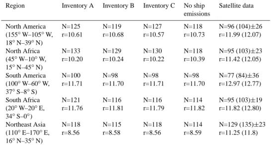
The cloud droplet number concentrations and effective cloud droplet radii simulated by the model are calculated from the annual mean of all grid cells in the regions spec-ified above, that are defined as ocean according to the T42 land-/sea-mask of E5/M1-MADE. The altitude range of the model data covers 0.6–1.1 km. Figure 5 shows the geograph-ical distributions of cloud droplet number concentration and cloud droplet effective radius over the ocean calculated by the model, which are used for intercomparison with the satel-lite data. Table 2 summarizes the model results using ship emission inventories A, B and C, as well as the model sim-ulation without ship emissions and the satellite data from MODIS and AMSR-E for average cloud droplet number con-centrations N and cloud droplet effective radii r. Error esti-mates for the cloud droplet number concentrations from the satellite data depend particularly on cloud fraction and liquid water path. For cloud fractions above 0.8 the relative retrieval error in cloud droplet number concentration is smaller than 80%, for small cloud fractions (<0.1), the errors in N can be up to 260% (Bennartz, 2007).
Basically, the model and satellite data show good agree-ment in cloud droplet number concentration. The model data
30 40 50 60 70 80 90 100
total cloud cover (%)
90°S 60°S 30°S 0°
latitude
30°N 60°N 90°N
ECHAM5/MESSy1-MADE (1999-2004) ISCCP (1983-2004)
Fig. 4. Multi-year zonal average of the total cloud cover calculated
by ECHAM5/MESSy1-MADE (solid) and obtained from ISCCP (International Satellite Cloud Climatology Project) satellite data for the period 1983–2004 (dashed; Rossow et al., 1996) in %.
lie mostly within the observed range spanned by the standard deviation and the results obtained from the satellite data ap-plying an alternative parameterization to retrieve the cloud droplet number concentration from measured effective radii and cloud optical thickness (Table 2). Bennartz (2007) con-cluded that marine boundary layer clouds even over the re-mote oceans have higher cloud droplet number concentra-tions in the Northern Hemisphere than in the Southern Hemi-sphere. This basic feature is reproduced by the model show-ing higher cloud droplet number concentrations over the
Pa-cific west of North America (118–127 cm−3)than over the
Pacific west of South America (98–100 cm−3) as well as
over the Atlantic west of North Africa (118–133 cm−3)than
over the Atlantic west of Southern Africa (114–121 cm−3).
Whereas the simulated cloud droplet number concentrations are in the upper range of the numbers given by the satellite data for all these oceanic regions, the simulated cloud droplet number concentrations are lower than observed over the Pa-cific east of Northeast Asia. This might indicate an under-estimation of Asian aerosol and precursor emissions in the model, which is consistent with the findings in Sect. 3.2 for the Aeronet measurement sites Kaashidoo and Male in the Indian Ocean.
The effective cloud droplet radii derived from the satel-lite data lie between 11 µm to 13 µm. Here the model gives slightly smaller values ranging from 10 µm to 11 µm for the regions North America, North Africa, South America, and Southern Africa. For the region Northeast Asia, the aver-age effective radii calculated by the model range from 8 µm to 9 µm, whereas the satellite data suggest 11 to 12 µm. Smaller cloud droplet radii and smaller cloud droplet num-ber concentrations indicate an underestimation of the liquid
Table 2. Annual average values for cloud droplet number concentrations N in cm−3and cloud droplet effective radii r in µm calculated by ECHAM5/MESSy1-MADE for low marine clouds (0.6–1.1 km) and derived from satellite data (Bennartz, 2007). Mean values with standard deviation are presented. The values in parentheses correspond to estimates derived from the satellite data using an alternative parameterization.
Region Inventory A Inventory B Inventory C No ship Satellite data
emissions North America N=125 N=119 N=127 N=118 N=96 (104)±26 (155◦W–105◦W, r=10.61 r=10.68 r=10.57 r=10.73 r=11.99 (12.07) 18◦N–39◦N) North Africa N=133 N=129 N=130 N=118 N=95 (103)±23 (45◦W–10◦W, r=10.20 r=10.24 r=10.22 r=10.39 r=11.42 (12.05) 15◦N–45◦N) South America N=100 N=98 N=98 N=98 N=77 (84)±36 (100◦W–60◦W, r=11.71 r=11.70 r=11.71 r=11.70 r=12.97 (12.77) 37◦S–8◦S) South Africa N=121 N=116 N=116 N=114 N=95 (103)±19 (20◦W–20◦E, r=11.76 r=11.81 r=11.79 r=11.82 r=11.82 (12.80) 34◦S–0◦) Northeast Asia N=118 N=115 N=118 N=114 N=129 (135)±23 (110◦E–170◦E, r=8.56 r=8.58 r=8.56 r=8.59 r=11.25 (11.8) 16◦N–35◦N) 180°W 180°W 120°W 120°W 60°W 60°W 0° 0° 60°E 60°E 120°E 120°E 180° 180° 60°S 60°S 0° 0° 60°N 60°N
cloud droplet number concentration
50 75 100 125 150 175 200 250 300 (cm-3) 180°W 180°W 120°W 120°W 60°W 60°W 0° 0° 60°E 60°E 120°E 120°E 180° 180° 60°S 60°S 0° 0° 60°N 60°N
cloud droplet effective radius
6 7 8 9 10 11 12 13 14
(µm)
Fig. 5. Multi-year average of the cloud droplet number concentration in cm−3(left) and cloud droplet effective radius in µm (right) over the ocean calculated by ECHAM5/MESSy1-MADE without ship emissions for model level 16 (0.6–1.1 km).
water content of low maritime clouds by the model in this region.
3.5 Cloud forcing
The cloud forcing is calculated as the difference between all-sky and clear-sky outgoing radiation at the top of the atmosphere (ToA) in the solar spectral range (shortwave cloud forcing) and in the thermal spectral range (longwave cloud forcing). The cloud forcing quantifies the impact of clouds on the radiation budget (negative or positive cloud forcings correspond to an energy loss and a cooling effect or an energy gain and warming effect, respectively).
Fig-ure 6 shows the zonally averaged annual mean short- and longwave cloud forcings calculated by E5/M1-MADE and obtained from ERBE (Earth Radiation Budget Experiment) satellite observations (Barkstrom, 1984) for the period 1985– 1989. E5/M1-MADE is able to reproduce the observed short-wave cloud forcing reasonably well, i.e. the model results lie mostly within the uncertainty range of the ERBE
measure-ments which is estimated to be about 5 W/m2. However, the
model tends to overestimate the observed values (absolute values) in particular near the two local maxima of the
short-wave cloud forcing at about 20◦N and 20◦S. Here,
devia-tions between model and satellite data reach up to 10 W/m2.
-100 -90 -80 -70 -60 -50 -40 -30 -20 -10 0
shortwave cloud forcing (W/m
2)
solar spectral range thermal spectral range
90°S 60°S 30°S 0° latitude 30°N 60°N 90°N 0 10 20 30 40 50
longwave cloud forcing (W/m
2) 90°S 60°S 30°S 0° latitude 30°N 60°N 90°N ERBE (1985-1989) ECHAM5/MESSy1-MADE (1999-2004)
Fig. 6. Multi-year zonal average of the top of the atmosphere (ToA) cloud forcing calculated by ECHAM5/MESSy1-MADE (solid) and
obtained from ERBE (Earth Radiation Budget Experiment) satellite observations for the period 1985–1989 (dashed; Barkstrom, 1984). The left panel shows the cloud forcing in the solar spectral range (shortwave cloud forcing), the right panel in the thermal spectral range (longwave cloud forcing) in W m−2.
marine stratocumuli as discussed in Sect. 3.4. It also affects the global annual averages. The model calculates a
short-wave cloud forcing of −52.9 W/m2, the ERBE satellite data
suggest a value of −47.4 W/m2.
The longwave cloud forcing calculated by E5/M1-MADE is in fairly good agreement with the ERBE observations, too. Differences between model and satellite data are
be-low 5 W/m2at most latitudes. The global annual averages of
the longwave cloud forcing are +28.0 W/m2(E5/M1-MADE)
and +29.3 W/m2(ERBE). However, the maximum shown in
the satellite data near the equator is not reproduced to its full extent by the model indicative of either insufficient high clouds or an underestimation of their altitude. Maximum
de-viations between model and satellite data of up to 12 W/m2
are found in this region.
4 Results
4.1 Contribution of shipping to the global aerosol
The dominant aerosol component resulting from ship
emis-sions is sulfate, which is formed by the oxidation of SO2
by the hydroxyl radical (OH) in the gas phase or by O3and
hydrogen peroxide (H2O2) in the aqueous phase of cloud
droplets. Depending on the ship emission inventory used, 2.3% (B,C) to 3.6% (A) of the total annual sulfate burden stems from shipping (Table 3). On average, 30–40% of the simulated sulfate mass concentration related to small parti-cles (<1 µm) near the surface above the main shipping routes originates from shipping (Fig. 7). In contrast, contributions are smaller for black carbon emissions from shipping (0.4%
in A to 1.4% in B) and particulate organic matter (0.1% in A to 1.1% in C), because the ship emission totals of both compounds are small compared to the contributions of fos-sil fuel combustion over the continents or to biomass
burn-ing. Despite high NOxemissions from shipping, the global
aerosol nitrate burden is only slightly increased by 0.1–0.2% using inventory A and B, but increased by 2.3% using
inven-tory C. Due to the lower average SO2 emissions in
inven-tory C compared to inveninven-tory A, less ammonium is bound
by SO4and thus more ammonium-nitrate forms. This results
in higher aerosol nitrate concentrations. Using inventory B, aerosol nitrate is lower than using inventory C despite low
SO2emissions. This is caused by the low NOxemissions in
inventory B compared to inventory C (Table 1). The increase in the water soluble compounds sulfate, nitrate and associ-ated ammonium causes an increase in the global burden of aerosol liquid water contained in the optically most active particles in the sub-micrometer size-range. This liquid wa-ter increase amounts to 4.3% (A), 2.2% (B), and 3.5% (C). Table 3 summarizes the total burdens and the relative contri-bution of shipping for the aerosol compounds considered in E5/M1-MADE for all three ship emission inventories.
The model calculates a ship induced increase in the parti-cle number concentration of the Aitken mode partiparti-cles (typ-ically smaller than 0.1 µm) of about 40% near the surface above the main shipping region in the Atlantic Ocean. Fur-thermore, the average geometric mean diameter of these par-ticles decreases from 0.05 µm to 0.04 µm as the freshly emit-ted particles from shipping are smaller than the aged Aitken particles typically found above the oceans far away from any continental source. Subsequent processes such as conden-sation of sulfuric acid vapor enable some particles to grow
180°W 180°W 120°W 120°W 60°W 60°W 0° 0° 60°E 60°E 120°E 120°E 180° 180° 60°S 60°S 0° 0° 60°N 60°N Inventory A 180°W 180°W 120°W 120°W 60°W 60°W 0° 0° 60°E 60°E 120°E 120°E 180° 180° 60°S 60°S 0° 0° 60°N 60°N Inventory B 180°W 180°W 120°W 120°W 60°W 60°W 0° 0° 60°E 60°E 120°E 120°E 180° 180° 60°S 60°S 0° 0° 60°N 60°N Inventory C -50 -45 -40 -35 -30 -25 -20 -15 -10 -5 0 5 10 15 20 25 30 35 40 45 50 (%)
Fig. 7. Simulated relative changes (annual mean) in % of near surface sulfate mass concentration in fine particles (<1 µm) due to shipping.
Left: ship emissions from inventory A (Eyring et al., 2005a), middle: inventory B (Dentener et al., 2006), right: inventory C (Wang et al., 20071).
Table 3. Global burden of aerosol compounds considered in ECHAM5/MESSy1-MADE and the contribution from international shipping in
the model simulations using the three emission inventories A (Eyring et al., 2005a), B (Dentener et al., 2006), and C (Wang et al., 20071).
Inventory A Inventory B Inventory C
Compound Atmospheric Contribution Atmospheric Contribution Atmospheric Contribution
Burden of Shipping Burden of Shipping Burden of Shipping
(Tg) (%) (Tg) (%) (Tg) (%) SO4 1.531 3.6 1.511 2.3 1.511 2.3 NH4 0.366 1.4 0.365 0.9 0.365 0.9 NO3 0.146 0.2 0.146 0.1 0.150 2.3 H2O 17.881 1.0 17.784 0.4 17.841 0.6 BC 0.119 0.4 0.122 1.4 0.119 0.8 POM 1.040 0.1 1.047 0.1 1.050 1.1 Sea Salt 3.588 – 3.582 – 3.589 – Mineral Dust 9.042 – 9.045 – 9.044 –
into the next larger size-range, the accumulation mode (0.1 to 1 µm), increasing the number concentration in this mode. Accumulation mode particles act as efficient condensation nuclei for cloud formation. The model results indicate that the accumulation mode particle number concentration in the lowermost boundary layer above the main shipping routes in the Atlantic Ocean is increased by about 15%. In contrast to the Aitken mode, the average modal mean diameter of the simulated accumulation mode is not affected by ship emis-sions and remains almost constant.
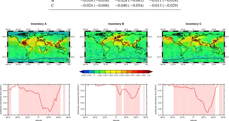
The changes in particle number concentration, particle composition and size-distribution result in an increase in aerosol optical thickness above the oceans of typically 2–3% (Fig. 8, upper row). Depending on the inventory used, dif-ferent amounts of emissions are assigned to specific regions. This leads to differences in the results: Individual regions such as the Gulf of Mexico show increases by up to 8–10% (A), the Northeastern Pacific by up to 6% (C), and the highly frequented shipping route through the Red Sea (Suez Canal) to the tip of India in the Indian Ocean by up to 10–14% (A,
B, C). This effect is mainly related to enhanced scattering of solar radiation by sulfate, nitrate, ammonium, and associated aerosol liquid water. The calculated changes in the global annual average clear-sky top of the atmosphere (ToA)
so-lar radiative flux are −0.038 W/m2 (A), −0.014 W/m2 (B),
and −0.029 W/m2 (C) (Table 4). Local changes of up to
−0.25 W/m2are simulated for the Gulf of Mexico (A), the Northeastern Pacific (C), or the highly frequented regions of the Indian Ocean (A, B, C). These regions can also be iden-tified in the zonal averages (Fig. 8, lower row). The contri-bution to changes in the clear-sky ToA thermal flux due to shipping is negligible and not statistically significant com-pared to its statistical fluctuations.
The changes in the simulated clear-sky fluxes do not rep-resent the global average direct aerosol forcing because the presence of clouds strongly modifies the aerosol impact on the radiation field. Small changes in cloud properties such as liquid water content, cloud droplet effective radius, or cloud cover between the model experiments with and without ship emissions are introduced not only because meteorology of
Table 4. Annual average changes in the top of the atmosphere (ToA) shortwave radiation flux (solar spectral range) due to direct aerosol
forcing (all-sky) from shipping in W m−2. The values in parentheses are the corresponding changes in the ToA shortwave clear-sky radiation flux.
Ship emission Pacific Ocean Atlantic Ocean Global
inventory (120◦E–80◦W, (75◦W–15◦E, mean
40◦S–60◦N) 40◦S–60◦N) A −0.033 (−0.072) −0.058 (−0.080) −0.011 (−0.038) B −0.016 (−0.038) −0.028 (−0.045) −0.011 (−0.014) C −0.024 (−0.048) −0.040 (−0.054) −0.013 (−0.029) Inventory A 180°W 180°W 120°W 120°W 60°W 60°W 0° 0° 60°E 60°E 120°E 120°E 180° 180° 60°S 60°S 0° 0° 60°N 60°N Inventory B 180°W 180°W 120°W 120°W 60°W 60°W 0° 0° 60°E 60°E 120°E 120°E 180° 180° 60°S 60°S 0° 0° 60°N 60°N -0.002 -0.001 0 0.001 0.002 0.003 0.004 0.005 0.006 0.007 0.008 0.009 0.01 Inventory C 180°W 180°W 120°W 120°W 60°W 60°W 0° 0° 60°E 60°E 120°E 120°E 180° 180° 60°S 60°S 0° 0° 60°N 60°N -0.10 -0.08 -0.06 -0.04 -0.02 -0.00 ∆
(clearsky shortwave flux) (W/m
2) 90°S 60°S 30°S 0° latitude 30°N 60°N 90°N -0.10 -0.08 -0.06 -0.04 -0.02 -0.00 ∆
(clearsky shortwave flux) (W/m
2) 90°S 60°S 30°S 0° latitude 30°N 60°N 90°N -0.10 -0.08 -0.06 -0.04 -0.02 -0.00 ∆
(clearsky shortwave flux) (W/m
2)
90°S 60°S 30°S 0° latitude
30°N 60°N 90°N
Fig. 8. Climatological annual mean (1999–2004) of changes in total aerosol optical thickness at 550 nm due to shipping (upper row) and
corresponding changes in the zonal mean shortwave clear-sky radiation flux at the top of the atmosphere (ToA) in W m−2(lower row). Hatched areas (upper row) and light-red shaded areas (lower row) show differences which are significant compared to the inter-annual variability.
each GCM simulation is not completely identical (random), but also because of modifications of cloud microphysical properties by ship emissions (systematic). These differences in cloud properties change the cloudy-sky ToA shortwave radiation even for identical aerosols. Thus, the calculated all-sky direct aerosol forcing results not only from changes in aerosol properties due to shipping, but also from differ-ent cloud properties. This prevdiffer-ents full separation of the di-rect and indidi-rect effect, which makes a comparison of the direct aerosol effect calculated for the different ship emis-sion inventories difficult. The all-sky direct aerosol forcing in each model simulation is calculated from the differences in the ToA all-sky solar radiation fluxes obtained with and without aerosols by calling the radiation module of the GCM twice. According to our model results, we estimate the
di-rect aerosol forcing from shipping to amount −0.011 W/m2
(A,B) to −0.013 W/m2 (C). The differences in the direct
aerosol forcing (all-sky) between the three ship emission in-ventories are smaller than expected from the emission totals (Table 1). This clearly indicates that the geographic distribu-tion of the emissions plays a key role for the impact of ship emissions on the radition budget. Table 4 summarizes the direct aerosol forcing from shipping calculated for the three emission inventories.
4.2 Modification of cloud microphysical properties
The second important effect of the aerosol changes due to ship emissions is a modification of cloud microphysical prop-erties. The model simulations reveal that this effect is mainly confined to the lower troposphere from the surface up to about 1.5 km. This implies that regions with a frequent high amount of low clouds above the oceans are most suscepti-ble for modifications due to ship emissions. Such regions
180°W 180°W 120°W 120°W 60°W 60°W 0° 0° 60°E 60°E 120°E 120°E 180° 180° 60°S 60°S 0° 0° 60°N 60°N 5 10 15 20 25 30 35 40 45 50 (%)
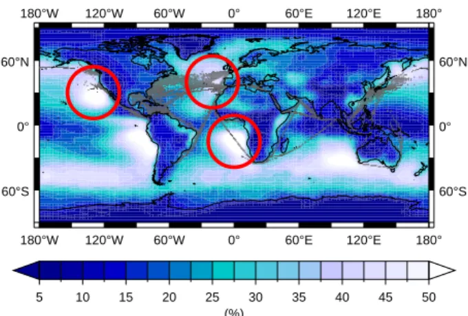
Fig. 9. Annual mean (1983–2004) low cloud amount (%) derived
from ISCCP (International Satellite Cloud Climatology Project) satellite data (Rossow et al., 1996). The highly frequented shipping routes (inventory A) are overlaid in gray. Regions with significant ship traffic (Eyring et al., 2005a) and high amount of low clouds are marked with red circles.
are coinciding with dense ship traffic over the Pacific Ocean west of North America, the Atlantic Ocean west of Southern Africa and the Northeastern Atlantic Ocean (Fig. 9). These regions are consistent with the locations showing the maxi-mum response in the indirect aerosol effect due to shipping calculated by E5/M1-MADE.
Whereas the vertically integrated cloud liquid water con-tent is only slightly (1–2%) affected by ship emissions and the ice crystal number concentration shows no significant change, simulated cloud droplet number concentrations are
significantly increased. Maximum changes of the cloud
droplet number are computed above the main shipping routes in the Atlantic and Pacific Ocean at an altitude of about 500 m. These changes in cloud droplet number
concentra-tion amount to 30–50 cm−3(20–30%) in the Atlantic (A, B,
C) and about 20–40 cm−3 (15–30%, A, C) and 5–15 cm−3
(5–10%, B) in the Pacific. Table 5 summarizes the annual average changes in cloud droplet number concentration and cloud droplet effective radius for the three ship emission in-ventories. The corresponding changes in cloud liquid wa-ter content at this altitude calculated by the model show an increase in the order of a few percent, but are statistically not significant. The increase in cloud droplet number causes a decrease in the effective radius of the cloud droplets. In the Atlantic Ocean, for instance, the average decrease in the cloud droplet effective radius is 0.42 µm (A), 0.17 µm (B), and 0.25 µm (C) at an altitude of 0.4 km (see also Table 5). This effect results in an enhanced reflectivity of these low marine clouds. This larger impact on average cloud droplet radii above the Atlantic by ship emissions from inventory A compared to inventories B and C cannot be explained by
the emission totals only. The emission total of SO2 from
inventory A (5.0 Tg/yr) is similar to that from inventory B
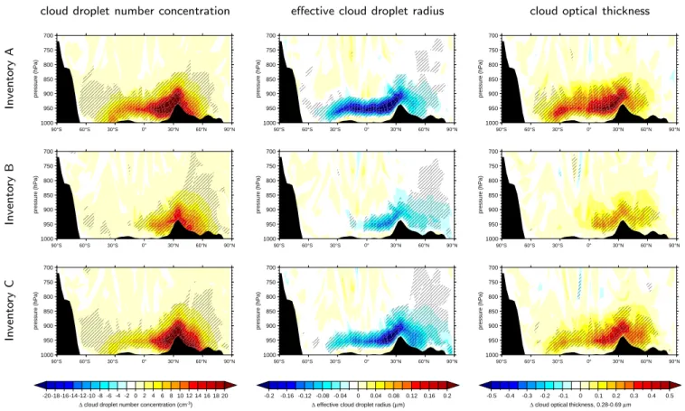
(4.7 Tg/yr). Again, this indicates that the geographic distri-bution of the emissions plays an important role: Emissions are much more widespread in inventory A compared to B, resulting in a larger impact on the cloud microphysical prop-erties averaged over a larger domain. Figure 10 depicts the annual mean changes in zonal average cloud droplet num-ber concentrations, cloud droplet effective radii, and cloud optical thickness in the spectral range 0.28–0.69 µm due to shipping for the three emission inventories. The increase in cloud droplet number concentration and the decrease in cloud droplet effective radii result in an increase in cloud optical thickness of typically 0.1 to 0.3 on zonal annual average. Whereas the changes in cloud optical thickness are limited
to the latitude range 0◦to 70◦N for inventory B, statistically
significant changes are calculated between 60◦S to 60◦N for
inventory A with maximum changes in cloud optical
thick-ness up to about 0.5 in the latitude range around 20◦N to
30◦N.
The simulated shipping-changes in the annual mean total cloud cover, the geographical precipitation patterns or the to-tal precipitation are statistically not significant compared to the inter-annual variability.
The increased reflectivity of the low marine clouds re-sults in an increased shortwave cloud forcing, calculated as the difference of the all-sky shortwave minus the clear-sky shortwave radiation at the ToA. The shortwave cloud forc-ing quantifies the impact of clouds on the Earth’s radiation budget in the solar spectral range. The changes in the cloud forcing include both, changes in the cloud reflectivity due to altered cloud droplet number concentration (1st indirect effect), as well as changes due to altered precipitation forma-tion efficiency (2nd indirect effect). However, no statistically significant changes in the precipitation patterns or total pre-cipitation have been encountered. Figure 11 shows the geo-graphical distribution of the 6-year annual average changes in ToA shortwave cloud forcing and the corresponding zonal means for the three ship emission inventories A, B, and C. Statistically significant changes in the shortwave cloud forc-ing are found in particular above the Pacific off the west coast of North America (A, C), the Northeastern Atlantic (A, B, C) and above the Atlantic off the west coast of Southern Africa (A, C). Local changes in the Pacific and Atlantic can reach
−3 to −5 W/m2 (A, C) and −2 to −3 W/m2 (B). In con-trast, changes above the Indian Ocean are smaller despite the high ship traffic density. This is due to the low cloud amount susceptible to ship emissions being rather low in this region (Fig. 9). Simulated changes in the longwave cloud forcing (thermal spectral range) are small and statistically not signif-icant because of the comparably low temperature differences between the sea surface temperature and the cloud top height of the low marine clouds. Changes in the zonally averaged annual mean cloud forcing for the solar spectrum due to ship
emissions are mostly confined to the latitude range 40◦S to
50◦N (A), 10◦N to 50◦N (B), and 30◦S to 50◦N (C).
cloud droplet number concentration effective cloud droplet radius cloud optical thickness In v e n to ry A 700 750 800 850 900 950 1000 pressure (hPa) 90°S 60°S 30°S 0° 30°N 60°N 90°N 700 750 800 850 900 950 1000 pressure (hPa) 90°S 60°S 30°S 0° 30°N 60°N 90°N 700 750 800 850 900 950 1000 pressure (hPa) 90°S 60°S 30°S 0° 30°N 60°N 90°N In v e n to ry B 700 750 800 850 900 950 1000 pressure (hPa) 90°S 60°S 30°S 0° 30°N 60°N 90°N 700 750 800 850 900 950 1000 pressure (hPa) 90°S 60°S 30°S 0° 30°N 60°N 90°N 700 750 800 850 900 950 1000 pressure (hPa) 90°S 60°S 30°S 0° 30°N 60°N 90°N In v e n to ry C 700 750 800 850 900 950 1000 pressure (hPa) 90°S 60°S 30°S 0° 30°N 60°N 90°N 700 750 800 850 900 950 1000 pressure (hPa) 90°S 60°S 30°S 0° 30°N 60°N 90°N 700 750 800 850 900 950 1000 pressure (hPa) 90°S 60°S 30°S 0° 30°N 60°N 90°N -20-18 -16-14-12-10 -8 -6 -4 -2 0 2 4 6 8 10 12 14 16 18 20
∆ cloud droplet number concentration (cm-3)
-0.2 -0.16 -0.12 -0.08 -0.04 0 0.04 0.08 0.12 0.16 0.2
∆ effective cloud droplet radius (µm)
-0.5 -0.4 -0.3 -0.2 -0.1 0 0.1 0.2 0.3 0.4 0.5
∆ cloud optical thickness, 0.28-0.69 µm
Fig. 10. Climatological annual mean (1999–2004) of zonally averaged changes in cloud droplet number concentrations (left), cloud droplet
effective radii (middle), and cloud optical thickness in the spectral range 0.28–0.69 µm (right) in the lower troposphere due to shipping. The upper row shows the changes calculated using ship emission inventory A (Eyring et al., 2005a), the middle row depicts changes calculated using ship emission inventory B (Dentener et al., 2006), the lower row shows changes calculated using ship emission inventory C (Wang et al., 20071). Hatched areas show differences which are significant at the 99% confidence level compared to their inter-annual variability.
Table 5. Annual average changes in cloud droplet number concentration (CDNC) and cloud droplet effective radius (r) due to shipping. The
numbers are given for model level 17 (0.3–0.6 km) for which the maximum sensitivity to shipping is simulated. The values in parentheses are given for model level 16 (0.6–1.1 km).
Inventory A Inventory B Inventory C
Region 1(CDNC) 1(r) 1(CDNC) 1(r) 1(CDNC) 1(r) (cm−3) (µm) (cm−3) (µm) (cm−3) (µm) Pacific Ocean 27.6 (6.7) −0.37 (−0.06) 13.7 (4.2) −0.15 (−0.03) 18.0 (4.4) −0.23 (−0.04) (120◦E–80◦W, 40◦S–60◦N) Atlantic Ocean 30.9 (8.2) −0.42 (−0.07) 15.5 (5.1) −0.17 (−0.04) 19.9 (5.4) −0.25 (−0.06) (75◦W–15◦E, 40◦S–60◦N) Global mean 13.6 (3.2) −0.18 (−0.02) 5.9 (1.8) −0.06 (−0.02) 10.4 (2.6) −0.13 (−0.03)
cloud forcing for all three emission inventories and different regions. The global annual mean changes in the shortwave
cloud forcing amount to −0.60 W/m2(A), −0.19 W/m2(B),
and −0.44 W/m2(C).
A comparison of the results with E5/M1-MADE simula-tions using pre-industrial emissions for trace gases (van Aar-denne et al., 2001) and particles (Dentener et al., 2006)
re-sults in a total anthropogenic indirect aerosol effect
(includ-ing ships) of −1.1 W/m2(B) to −1.5 W/m2(A). These
val-ues are within the range of previous model estimates (−0.9
to −2.9 W/m2)(Lohmann and Feichter, 2005) of the total
an-thropogenic indirect effect. The fourth assessment report of the Intergovernmental Panel on Climate Change (IPCC) re-ports a best estimate for the cloud albedo effect (1st indirect
Inventory A 180°W 180°W 120°W 120°W 60°W 60°W 0° 0° 60°E 60°E 120°E 120°E 180° 180° 60°S 60°S 0° 0° 60°N 60°N Inventory B 180°W 180°W 120°W 120°W 60°W 60°W 0° 0° 60°E 60°E 120°E 120°E 180° 180° 60°S 60°S 0° 0° 60°N 60°N -2.5 -2 -1.5 -1 -0.5 0 0.5 1 1.5 2 2.5 (W/m2) Inventory C 180°W 180°W 120°W 120°W 60°W 60°W 0° 0° 60°E 60°E 120°E 120°E 180° 180° 60°S 60°S 0° 0° 60°N 60°N -1.2 -1.0 -0.8 -0.6 -0.4 -0.2 -0.0 ∆
(shortwave cloud forcing) (W/m
2) 90°S 60°S 30°S 0° latitude 30°N 60°N 90°N -1.2 -1.0 -0.8 -0.6 -0.4 -0.2 -0.0 ∆
(shortwave cloud forcing) (W/m
2) 90°S 60°S 30°S 0° latitude 30°N 60°N 90°N -1.2 -1.0 -0.8 -0.6 -0.4 -0.2 -0.0 ∆
(shortwave cloud forcing) (W/m
2)
90°S 60°S 30°S 0° latitude
30°N 60°N 90°N
Fig. 11. Multi-year average of simulated changes in shortwave cloud forcing due to shipping at the top of the atmosphere (ToA) in W m−2. Upper row shows the geographical distribution, lower row zonal averages. Hatched areas (upper row) and light-red shaded areas (lower row) show differences which are significant at the 99% confidence level compared to the inter-annual variability.
Table 6. Annual average changes in the top of the atmosphere
(ToA) shortwave cloud forcing (solar spectral range) due to ship emissions in W m−2.
Ship emission Pacific Ocean Atlantic Ocean Global inventory (120◦E–80◦W, (75◦W–15◦E, mean
40◦S–60◦N) 40◦S–60◦N)
A −1.22 −1.46 −0.60
B −0.46 −0.60 −0.19 C −0.77 −0.93 −0.44
aerosol effect) of −0.7 W/m2 with a 5% to 95% range of
−0.3 to −1.8 W/m2 (IPCC, 2007). The results of
E5M1-MADE (−1.1 to −1.5 W/m2) are in the upper range of these
uncertainties. However, it should be kept in mind, that most models consider ships in a simplified manner such as tory B only. Thus, the total indirect forcing using
inven-tory B (−1.1 W/m2) should be considered only when
com-paring E5M1-MADE to the IPCC results. According to the results of our model studies, shipping contributes to about 17% (B) to 39% (A) of the total anthropogenic indirect effect. This contribution is larger than the contribution of shipping to aerosol emissions, because of larger albedo changes by clouds over dark oceans than over land. In addition, this ef-fect is comparatively large since ship emissions are released in regions with frequent occurrence of low clouds, which are highly susceptible to the enhanced aerosol number con-centration in an otherwise clean marine environment. For
both reasons, the susceptibility of the radiation budget to ship emissions is much higher than for continental anthropogenic aerosol sources of the same source strength. Simple scal-ing of the total anthropogenic indirect aerosol effect to the contribution of an individual source to the total atmospheric burden is therefore questionable for shipping.
4.3 Radiative forcing due to international shipping
The indirect aerosol effect of shipping on climate discussed in Sect. 4.2 results in a negative radiative forcing (RF) which is, in absolute numbers, much higher than the negative RF caused by the scattering and absorption of solar radiation by aerosol particles (direct aerosol effect) or the positive RF due to greenhouse gases, mainly carbon dioxide and ozone
(Fig. 12). NOx and other ozone precursor emissions from
shipping not only perturb the atmosphere by the formation
of O3, but also lead to enhanced levels of OH, increasing
removal rates of CH4, thus generating a negative radiative
forcing. These previously estimated forcings are all in the
range of ±15 to 50 mW/m2 (Endresen et al., 2003; Eyring
et al., 2007). RF due to direct CH4from shipping (0.52 Tg
CH4from fuel and tanker loading; Eyring et al., 2005a) has
not been estimated so far. However, because of the small
contribution (<0.2%) to total anthropogenic CH4emissions
(Olivier et al., 2005), the resulting forcings are expected to be negligible compared to the other components.
Fig-ure 12 shows the RF due to shipping from CO2, O3, CH4,
and the direct effect of SO4 particles from Endresen et al.
(2003) and Eyring et al. (2007) as well as the radiative forc-ing due to ship tracks (Schreier et al., 2007) in comparison
to the estimated direct aerosol effect (Sect. 4.1) and indirect aerosol effect (Sect. 4.2) obtained in this study for the three ship emission inventories A, B, and C. Schreier et al. (2006) showed that ship tracks can change the radiation budget on a local scale, but are short lived and cover a very small frac-tion of the globe so that their radiative effect on the global
scale is negligible (−0.4 to −0.6 mW/m2±40%; Schreier et
al., 2007). Ship tracks are changes in cloud reflectance due to ship emissions, which are detectable in satellite data and are identified by elongated structures. In contrast, this study investigates particularly the large scale effects of ship
emis-sions on clouds, after for instance SO2 is oxidized to
sul-fate and emissions are spread out far over the ocean, which are not covered by an investigation of pure ship tracks. The contribution of water vapor emissions from shipping is also negligible. Also shown is a previous estimate by Capaldo et al. (1999), who used a global model without detailed aerosol microphysics and aerosol-cloud interaction and assessed the
first indirect effect of SO4 plus organic material particles
(−0.11 W/m2). In contrast to Capaldo et al. (1999), Endresen
et al. (2003) and Eyring et al. (2007), the model study pre-sented here considers not only sulfate, but changes in the ra-diation budget due to the sum of all relevant aerosol
compo-nents (SO4, NO3, NH4, BC, POM, and aerosol liquid water).
The model results discussed in Sects. 4.1 and 4.2 and shown in Fig. 12 also indicate that the geographical distri-bution of emissions over the globe plays a key role deter-mining the global impact of shipping. The large differences in the model results obtained with three different ship emis-sion inventories (Eyring et al., 2005a; Dentener et al., 2006,
Wang et al., 20071) imply a high uncertainty, but on the other
hand the main conclusions of this study hold for all three in-ventories. For all inventories used, the present-day net RF from ocean-going ships is strongly negative, in contrast to, for instance, estimates of RF from aircraft, ranging from
0.048 to 0.071 W/m2(without cirrus) and 0.03 W/m2(0.01 to
0.08 W/m2) for aviation-induced cirrus (Sausen et al., 2005).
In addition, the direct aerosol forcing due to scattering and absorption of solar light by particles from shipping is only of minor importance compared to the indirect aerosol effect. Additional sensitivity simulations with sulfur free fuel with E5/M1-MADE revealed that about 75% of the direct and in-direct aerosol effect from shipping is related to the fuel sulfur content, which is currently about 2.4% (EPA, 2002). Thus, a simple upscaling of the results from Capaldo et al. (1999) to the total indirect effect considering all relevant aerosol
com-pounds from shipping results in about −0.15 W/m2. This
value is comparable to the indirect aerosol effect calculated
in this study using inventory B (−0.19 W/m2). Inventory B
has similar emission totals for SO2(7.8 Tg yr−1)as the ship
emission inventory used by Capaldo et al. (1999) totaling
8.4 Tg yr−1. -600 -550 -500 -450 -400 -350 -300 -250 -200 -150 -100 -50 0 50 RF [mW/m 2] Ship RF A B C -0.4 mW/m2 A B C
CO2 O3 CH4 Direct Indirect Ship Tracks from NOx
Level of scientific understanding
Good Fair Fair Fair Poor Poor
Endresen et al., 2003 Eyring et al., 2007
Capaldo et al., 1999 this study (inventory A/B/C) Schreier et al., 2007
Fig. 12. Annual mean radiative forcing due to emissions from
inter-national shipping in mW m−2. Values for CO2, O3, CH4(reduced lifetime), and SO4(direct aerosol effect) are taken from Endresen et al. (2003) and Eyring et al. (2007). The indirect aerosol effect cal-culated by Capaldo et al. (1999) includes the first indirect effect of sulfate plus organic material aerosols only, the error bar depicts the range spanned by their additional sensitivity studies. The estimated direct and the indirect aerosol effect calculated in this study also includes changes due to BC, POM, NH4, NO3, and H2O from ship-ping in addition to SO4and refers to the changes in all-sky short-wave radiation fluxes and net cloud forcing (sum of shortshort-wave and longwave cloud forcing) at the top of the atmosphere, respectively. The net cloud forcing is calculated from the differences in the sim-ulated all-sky fluxes and the corresponding clear-sky fluxes at top of the atmosphere. The global annual mean RF due to ship tracks is taken from the satellite data analysis by Schreier et al. (2007). For details see text.
5 Summary and conclusions
In this study we used the atmospheric general circulation model ECHAM5/MESSy1 coupled to the aerosol module MADE (E5/M1-MADE) to study the impact of shipping on aerosols, clouds and the Earth’s radiation budget. The aerosols calculated by E5/M1-MADE are used to drive the radiation and cloud scheme of the GCM, allowing the assess-ment of both, the direct and indirect aerosol effect of emis-sions from shipping. The evaluation of the model showed that the main features of the observed geographical patterns, seasonal cycle and vertical distribution of the basic aerosol parameters are captured. However, the comparison also un-veiled existing weaknesses of the model, such as represent-ing the optical properties of mineral dust or capturrepresent-ing Asian emissions of particulate matter and aerosol precursors. For the purpose of this study, these model deficiencies are ac-ceptable when assessing the impact of shipping on aerosols and clouds by calculating differences between model simu-lations with and without ship emissions.
To assess uncertainties in estimates of present-day (year 2000 conditions) emission totals and spatial ship traffic