HAL Id: hal-01342928
https://hal.univ-lorraine.fr/hal-01342928v2
Submitted on 4 Aug 2016
HAL is a multi-disciplinary open access
archive for the deposit and dissemination of sci-entific research documents, whether they are pub-lished or not. The documents may come from teaching and research institutions in France or abroad, or from public or private research centers.
L’archive ouverte pluridisciplinaire HAL, est destinée au dépôt et à la diffusion de documents scientifiques de niveau recherche, publiés ou non, émanant des établissements d’enseignement et de recherche français ou étrangers, des laboratoires publics ou privés.
Basin, Turkey
Pauline Collon, Alexandre Pichat, Charlie Kergaravat, Arnaud Botella,
Guillaume Caumon, Jean-Claude Ringenbach, Jean-Paul Callot
To cite this version:
Pauline Collon, Alexandre Pichat, Charlie Kergaravat, Arnaud Botella, Guillaume Caumon, et al.. 3D modelling from outcrop data in a salt tectonic context: Example from the Inceyol mini-basin, Sivas Basin, Turkey. Interpretation, SAGE Publications, 2016, 4 (3), pp.SM17-SM31. �10.1190/INT-2015-0178.1�. �hal-01342928v2�
Collon P., Pichat A., Kergaravat C., Botella A., Caumon G., Ringenbach J.C. , Callot J.P. (2016). 3D modelling from outcrop data in a salt tectonic context : Example from the Inceyol mini-basin, Sivas Basin, Turkey. Interpretation, Vol. 4(3), pp. SM17−SM31.
3D modelling from outcrop data in a salt tectonic context:
Example from the Inceyol mini-basin, Sivas Basin, Turkey.
Pauline Collon∗, Alexandre Pichat†‡, Charlie Kergaravat†‡, Arnaud Botella∗§, Guillaume Caumon∗, Jean-Claude Ringenbach† and Jean-Paul Callot‡
ABSTRACT
We propose a 3D modelling strategy of the encased mini-basin of Inceyol in Sivas (Turkey). The challenge lies in the combination of sparse outcrop data and the com-plex interpretive geometry of geological structures that comes from salt tectonics. We succeeded in modelling the convoluted salt surface using an explicit indirect surface patch construction method followed by a manual mesh improvement. Then, we mod-elled the mini-basin sediments with an implicit approach. The result highlights the remarkable geometry of the convoluted salt horizon and its associated mini-basin by extending in 3D the geologist’s interpretive 2D sections. This case study proves that building complex geometries is feasible with the existing tools and a good expertise in the various geomodelling techniques. The work also underlines the need for new methods to ease the modelling of such tectonic features from sparse data. We propose a 3D view of the model thanks to WebGL technology, as well as downloadable data to constitute a reference case study.
INTRODUCTION
Salt plays a significant role in tectonic, thermal and fluid migration processes owing to its peculiar physical properties, and especially so in hydrocarbon trap formation (e.g., Fossen, 2010). Economic interests associated with halokinesis have motivated a large number of studies to increase knowledge of the geometry of diapiric features at depth (e.g., Hudec and Jackson, 2007; Rowan et al., 2014) and the associated tectonic mechanisms (e.g., Vendeville et al., 1995; Giles and Rowan, 2012; Rowan and Vendeville, 2006). These studies demon-strate a large variety of halokinetic structures and highlight ambiguities in interpreting conventional seismic images (e.g., Fossen, 2010; Jackson et al., 2014). To help their un-derstanding, outcrop analogues are precious and sought after. They are the only way to get a direct 2D observation of many sub-seismic evaporite-related geometries. Sometimes, particular outcropping conditions even allow access to some 3D geometries. This knowledge
strongly helps the interpretation of structures poorly imaged by reflection seismic data (e.g., Giles and Lawton, 2002; Jackson and Harrison, 2006; Ringenbach et al., 2013; Callot et al., 2014).
In addition to field work, quantitative 3D modelling can help understanding of the three-dimensional organization of halokinetic features. Their complex geometry is indeed not eas-ily assessed by 2D cross-sections only. Moreover, quantitative 3D models further clear the way to numerical simulations as, e.g., structural restoration or constrained potential field inversion (e.g., Back´e et al., 2010; Lindsay et al., 2012). Building 3D models essentially calls for interpolation and/or extrapolation techniques. This is generally achieved by cre-ating smooth surfaces between data (e.g., Caumon et al., 2009). There are, however, many different and complex features in salt tectonics, mostly because salt deformation and migra-tion do not particularly generate minimal surfaces (e.g., Giles and Lawton, 2002; Jackson and Harrison, 2006; Fossen, 2010). This probably partly explains why no formal modelling framework has yet been defined for this specific environment, making extrapolation of salt geometry particularly challenging and interpretive in sparse data settings. Trocm´e et al. (2011) have proposed a 3D structural model of the southern Zagros diapiric province (Ja-hani et al., 2009). Using a large amount of data - ranging from geological surface data, such as outcrop surveys and dip measurements, to subsurface information coming from seismic interpretations and well wireline data - they used an explicit surface-based struc-tural modelling approach to provide a 3D regional model of the area. The large scale of their study limited the halokinetic features that could be represented in the model. This work also highlighted the limitations of explicit approaches in relation to modelling coherent stratigraphic formations when data are sparse. The implicit stratigraphic model building protocol proposed by Caumon et al. (2013) eases this task while providing some tools to directly exploit 3D geomorphologic features in stratigraphic interpolation. The application of the implicit stratigraphic modelling method to La Popa Basin in Mexico (Caumon et al., 2013), however, generated also a regional model that locally simplified the actual geometry of the diapiric structures and of the associated stratigraphy.
Figure 1: Geomodelling workflow adopted in this case study.
In this paper, we focus on the Inceyol mini-basin located in the Sivas Basin, Turkey. The high quality but sparse information and the complex geometries observed at outcrop present a real challenge for 3D geological model building. Our purpose is mainly to demonstrate the
feasibility of such a 3D modelling task. After modelling the salt surface using an explicit indirect surface patch construction method, we used an implicit method for the mini-basin sedimentary deposits. This required an intermediate step of volumetric mesh generation (Fig. 1). As only outcrop data are available, extrapolation at depth is bound to be quite concept-driven. Our result is a coherent 3D model reflecting the interpretive scenario of salt infill. It constitutes a necessary basis for further quantitative studies (e.g., implying potential field data or for uncertainty management). Finally, we discuss challenges and avenues to more objectively address 3D modelling in salt-tectonic context.
THE INCEYOL MINI-BASIN: GEOLOGICAL SETTING
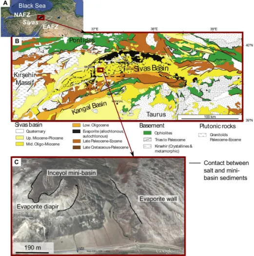
Located in the Central Anatolian Plateau, Turkey (Fig. 2A), the Sivas Basin formed from the Paleocene to the Pliocene in a foreland fold-and-thrust belt basin setting (Kurtman, 1973; Cater et al., 1991; Guezou et al., 1996; Poisson and Guezou, 1996; G¨undogan et al., 2005). At the end of the Eocene, a huge accumulation of marine evaporitic deposits occurred in the Sivas Basin. Their deformation accommodated the development of several kilometric-scale continental to marine mini-basins of Oligo-Miocene age. Striking evidences of such halokinetic structures are well observed in the central part of the Sivas Basin which exhibits a typical wall and basin structure (WABS) characterized by mini-basins surrounded by polygonal network of evaporite walls and welds (Ringenbach et al., 2013; Callot et al., 2014; Ribes et al., 2015, 2016; Kergaravat, 2016). Mini-basins exhibit several salt tectonic structures, such as halokinetic sequences, resulting from the interplay between sediment accumulation and salt flow (Ribes et al., 2015, 2016; Kergaravat, 2016).
The Inceyol mini-basin is located in the central WABS domain of the Sivas basin (Fig. 2B-C). It belongs to a set of several small-scale encapsulated secondary mini-basins that developed within a north/south regional compressional setting over deflating diapiric struc-tures (Kergaravat, 2016; Ribes et al., 2016). The Inceyol mini-basin is approximately 700 m wide by 800 m long. It is filled by more than 300 meters of saline lacustrine to sebkhaic deposits of Oligocene age. The mini-basin is structured as an encased system of synclinal folds displaying an elliptical shape in overall outline (Fig. 3). It is surrounded on its north, east and west borders by diapiric evaporites along which strata are strongly rotated into sub-vertical or locally overturned orientations (Pichat et al., 2015; Kergaravat, 2016). On its south and south eastern parts, landslides made of gypsum screes cover the mini-basin sediments (Fig. 4A). The diapiric evaporites are characterized by a chaotic amalgamation of massive gypsum to anhydrite blocks and mega blocks, more or less sheared to brecciated and mixed with red to green clays (Fig. 4A-C). Locally, diapiric structures also display brecciated to well bedded crystalline gypsum (selenitic facies) (Pichat et al., 2015). In diapirs, measurements of bedding (S0) and schistosity (S1) are most often parallel to the
neighbouring salt/sediment contacts. We could only observe two salt-sediment contacts correctly, mainly due to the combination of landslides, meteoritic alteration, brecciation and vegetation cover. On these places, the diapir-sediment contact displays a centimeter to meter-thick shear zone in which clasts and slivers of gypsum/anhydrite are embedded in a shale gouge affected by several fractures filled with satin-spar gypsum (Figure 4B).
In detail, the Inceyol mini-basin forms a single syncline in the north that splits to the south into two individualized tight synclines (Fig. 3A-B). The two synclines are separated by an exposed gypsum wall, interpreted at depth as a weld or a thin wall. At the outcrop,
Contact between salt and mini-basin sediments
Figure 2: Location of the Sivas basin and the Inceyol mini-basin. A - Tectonic map of Turkey, with the main continental blocks, major suture zones and Oligo-Miocene Sivas Basin deposits (adapted from Ribes et al. (2015)). B - Location of the Inceyol mini-basin in the geological setting of the Sivas Basin (Geological map adapted from Ringenbach et al. (2013)). C - Satellite image (Google Earth) of the Inceyol mini-basin on which the salt/sediment contact can be identified.
Figure 3: The Inceyol encased mini-basin (MB): geological conceptual model (Kergaravat, 2016). A - Map view showing the location of the AA’ cross-section and of the photography B. B - Photography of the mini-basin taken from the south and showing the splitting of the mini-basin by an exposed gypsum wall. C - AA’ Cross-section: one interpretation of the mini-basin at depth (Kergaravat, 2016).
both sides of the salt wall are marked by steep to overturned flanking strata (Fig. 3C). The strong dip variations across the synclines highlight the progressive rotation of the mini-basin flanks, which we interpreted as a syn-sedimentary mini-mini-basin subsidence during the salt flow (Kergaravat, 2016). Dip measurements in the sediments are difficult to determine at the immediate proximity of the salt-sediment contact due to the previously described alteration. Thus, we extrapolated the contact angles between salt and sediments from the closest measurements. A discordant contact seems to be dominant along the central diapir that splits the mini-basin. At the outer boundaries of the mini-basin, dip measurements indicate a more conformable salt-sediment contact.
In more detail, small normal faults cut the strata in the two synclines with an estimated throw less than 2-3 m (Fig. 3A). We also observed equivalent local reverse faults in the core of the eastern syncline. Small scale folding occurs in some sebkhaic deposits and are believed to accommodate flexure. Finally, along the eastern border of the basin, the observation of one strata overturned more than 180◦ could possibly highlight a halokinetic sequence (Figure 4A). Nevertheless, the outcrop quality prevented clear definition of the geometry of the structure and no other observation allowed us to extrapolate it elsewhere in the mini-basin.
Diap
ir-se
dim
ent
cont
act
Landslide
Overturned
strata
A
B
C
B Massive diapiric gypsum Diapiric gypsum 1 mShear zone
Mini-basin sedimentsE
W
Figure 4: A - Overturned lacustrine deposits against the eastern bordering diapiric wall. B - Focus on the diapir-sediment contact marked by a shale gouge in which are embedded reworked diapiric gypsum clasts. C - Diapiric breccia of massive gypsum/anhydrite.
METHODOLOGY
Field geologists first deemed the Inceyol geological structures to be too complex to model in 3D. Our objectives were to find one way to succeed and identify future numerical de-velopments that would ease the modelling of halokinetic features. To extend in 3D the 2D interpretations of geologists, we decided to use the simplest topological interpretation for the mini-basin compatible with the modelling scale and the field observations. It corre-sponds to the cross-section in Figure 3C. The mini-basin sediments are so interpreted as conformable to the salt boundary on the external part and at depth, but with a discordant contact along the central gypsum wall. We decided also to ignore the small-scale features like the small faults and folds observed in the sediments, as well as the overturned strata observed along the eastern border of the mini-basin for which no clear geometry was stated. Their dimensions are indeed below the current resolution of the model, which is 10 m for the sediments.
We built the model with the Skua-Gocad geomodelling software∗, StructuralLab (Frank et al., 2007; Caumon et al., 2013) and GoPy (Antoine and Caumon, 2008) research plugins, and the VorteXLIB library (Botella et al., 2014). The global workflow, calling for various techniques, consists in four main steps (Fig. 1). After data collection and integration into the geomodelling software, we built the triangulated surface corresponding to the salt top with an explicit indirect surface construction method. Then, we generated a 3D volumetric mesh conformable to this salt surface. Last, we reconstructed the sedimentary filling of the mini-basin with an implicit surface modelling method.
Data and information
Available data to model the Inceyol mini-basin are a Digital Elevation Model (DEM), satellite images and strata orientation measurements. The covered area extends over 980 m North-South and 1080 m East-West (Fig. 5). These data are complemented with interpre-tive cross-sections (e.g., Fig. 3C). To ensure spatial coherency, all data were georeferenced in the Universal Transverse Mercator projection (UTM - Zone 37) in the World Geodetic System 1984 (WGS84). To allow further use of this case study, dip measurements, DEM, satellite images and interpreted curves of the stratigraphic levels and of the salt boundary are all available for download on the RING team website†.
Digital Elevation Model The Digital Elevation Model (DEM) used in this work has a 5 m horizontal resolution and an around 50 cm vertical precision. In the zone of interest, elevation ranges between 1,348 m and 1,595 m. We imported the DEM into the Skua-Gocad geomodelling software as a point set and we reconstructed the topographic surface by connecting all these points by a Delaunay triangulation.
Interpreted satellite images Satellite images were extracted from an ArcGis Web Map Service‡, maintained by the Open Geospatial Consortium. They were imported,
georefer-∗http://www.pdgm.com/products/skua-gocad/
†http://ring.georessources.univ-lorraine.fr/ring dl/public/models/Sivas onLine Data.zip ‡http://services.arcgisonline.com/arcgis/rest/services
enced and vertically projected on the topographic surface. We interpreted these images to provide a set of curves corresponding to: i) the salt/sediment contact and ii) the strati-graphic traces (Fig. 5B).
Orientation measurements 76 stratigraphic orientation measurements were taken in the field. These data points were positioned using a GPS system with a precision close to 1 meter. We integrated them directly as a pointset containing the strike (right-hand convention) and dip properties. The normal vectors to the stratigraphic surfaces were then computed from azimuth and dip and constitute a 3D vector property associated to each point (Fig. 5A).
Dip measurements Salt contour Salt contour stratal traces DEM Satellite image 1090 m 980 m
Figure 5: Outcrop data : we realized the modelling using a 5 m resolution DEM (black lines each 50 m), 76 dip measurements of strata, salt contours and stratigraphic lines interpreted from a satellite image.
Conceptual model From outcrop data only, geomodel building is clearly an under-constrained problem and the extrapolation at depth is bound to be quite concept-driven. Thus, we completed the field dataset with interpretive cross-sections of the mini-basin, il-lustrating the conceptual geometries at depth. The cross-section presented in Figure 3C was imported in the geomodelling software and georeferenced. Interpretation lines were digitized from this section and then used as a guide for the 3D model construction (Fig. 6). Three other cross-sections were georeferenced and reinterpreted directly in 3D. Over-all, we created 3 East-West and 2 North-South numerical cross-sections. Their geological interpretations are based on the observation of similar structures imaged by seismic data
(Ringenbach et al., 2013) and on our local knowledge of halokinetic structures in the Sivas Basin (Ringenbach et al., 2013; Callot et al., 2014; Ribes et al., 2015, 2016; Pichat et al., 2015). In particular, we supposed that the mini-basin is approximately 300 m deep on the eastern part, and 150 m deep on the western part. To ensure consistency with dip mea-surements and similarity with the other mini-basins observed in the Sivas area, we assumed both eastern and western parts to have a particular coin purse shape.
Salt boundary Interpretive data Topographic surface 1090 m 960 m 800 m
Figure 6: Data points used to model the salt surface: red lines are interpretive data coming from the geological conceptual model.
Modelling choices
Various techniques exist for modelling geological interfaces like horizons and faults. They can be classified in two main strategies (e.g. Frank et al., 2007; Caumon et al., 2009; Collon et al., 2015): i) the classical modelling approaches, also called explicit approaches, which consist in building surfaces - generally triangulated surfaces - that fit available data; ii) and the more recent implicit approaches, which consider geological interfaces as isovalues of a 3D scalar field f (x, y, z). In this work, to compute the scalar field, we used an optimisation method that consists in minimising a weighted sum of various constraints including the data misfit (Frank et al., 2007; Caumon et al., 2013).
Implicit approaches automatically prevent overlapping or leaking layers. But at the same time, the 3D scalar field continuity can only handle conformable stratigraphic blocks: each discontinuity implies a new 3D scalar field definition that is interpolated independently of the previous one. Thus, the discordant salt-sediment contacts observed along the central diapir require separate consideration of the salt surface from the mini-basin sedimentary deposits.
Modelling the salt surface
With only 5 numerical cross-sections and a particularly convoluted shape, the construction of a salt surface that fits the geological interpretation is quite challenging. We tested two approaches for this purpose.
Implicit approach
Each digitized curve was used as a constraining data to interpolate a 3D scalar field f (x, y, z) on the whole volume of interest in an implicit approach. Here, we used a discrete interpo-lation scheme, meaning that the scalar field is defined by a piece-wise linear interpointerpo-lation of the values stored at the vertices of a tetrahedral mesh. Once this 3D scalar field is computed, any stratigraphic surface can be explicitly constructed by extracting the corre-sponding isovalue surface. We defined the salt surface to be reconstructed as the implicit surface corresponding to f (x, y, z) = 0.
First, we built a surface with digitized curves as the only constraint using the Skua-Gocad Structure & Stratigraphy workflow. The resulting surface honours the line data, but has a complex topology with diapir-shaped mini-basin geometry that is inconsistent with our interpretation (Fig. 7).
C
B
A C
Figure 7: Implicit modelling of the salt surface with digitized curve constraints alone. Image A, B, C show models built with volumetric mesh resolutions of 10 m (A), 20 m (B) and 30 m (C).
Secondly, polarity information was added using the implicit method implemented in the StructuralLab Skua-Gocad research plugin, which includes the possibility to impose inequality constraints as defined by Frank et al. (2007). Two vertical surfaces were manually built in the center of both mini-basin synclines (Fig. 8A). We attached a Greater than constraint to each of these surfaces. Two inequality control points, chosen arbitrarily on each side of the surface to build, were also used: one with the constraint f (x, y, z) ≥ 5 and the other one with the constraint f (x, y, z) ≤ −5. The scalar field was computed on a tetrahedral mesh made of 545,642 tetrahedra corresponding to a 30 m average tetrahedron edge length. Note that we performed a similar computation with a finer mesh (2,162,146 tetrahedra for an average tetrahedron edge length of 18 m) without noticeable differences in the results but a significant increase of memory cost and computation time (passing from approximately 1 min to 3.5 h for the scalar field computation). With such additional constraints, the resulting salt surface is clearly improved with a global shape closer to the geological interpretation (Fig. 8B). In detail, however, the result still shows some unsatisfactory parts (Fig. 8C-D-E).
First, when the salt boundary is not clearly visible at outcrop - and thus imposed by a digitized curve -, the salt surface is smoothed and looses its purse shape (Fig. 8C). This is completely consistent with the interpolation principle that minimizes the variations of the scalar field gradient (Frank et al., 2007): if no data “forces” the surface to twist, the surface
A B
Figure 8: Implicit modelling of the salt surface with inequality constraints. A - Additional information used to impose the surface polarity: two surfaces are defined inside the mini-basin as well as one point (in red). They are attached to a Greater than constraint (Frank et al., 2007). One point is used at depth (in blue) to define the other side of the surface using a Less than constraint. B - Result obtained using a volumetric tessellation of 30 m resolution. C - Top view and zoom on the model B. D - Bottom view on the central diapir showing the local fusion of the two sides and the artefacts due to mesh resolution. E - Side view on the central diapir highlighting the unwanted “hole” in the salt. F - Additional curves used to force the interpolation to close this hole and corresponding result (G).
tends to be planar, whereas interpretation would suggest locally cylindrical structures. This is also observed at the edge of the domain of interest: in the southern part the surface tends to plunge at depth instead of keeping a flat bottom; no flattening is obtained either on the aerial (eroded) parts. Moreover a protuberance is produced at outcrop in the South-East because the outcropping salt boundary changes its orientation (Fig. 8B). To avoid this, additional interpretive curves should be added on the topography, at depth and above the topography, iteratively, until the computed result would be satisfactory.
Second, the central diapir is not well modelled and a hole appears in the salt wall (Fig. 8E). Locally, the two sides of this central diapir also locally vanish, which is visible when looking from bottom (Fig. 8D). Indeed, the outcrop data indicate a progressive closure of the salt wall and, at this location, the distance between the two sides is lower than 30 m. Two reasons explain this result: the volumetric mesh resolution that is equivalent to this distance and, again, the polarity of the surface that is locally under-constrained. To solve this last issue, we made a last try by adding two curves representing the salt neck (Fig. 8F). Unfortunately, it only managed to close partially the hole (Fig. 8G). Nonetheless, the thinness of this zone could ultimately be managed with an adaptive mesh comprising smaller tetrahedra or incoparating an explicit salt weld in this zone. There also, iterative addition of constraining data would again be necessary to obtain the desired representation.
Explicit approach
To more directly obtain a salt model whose topology matches our interpretation, we finally chose to use an explicit modelling method. Its principle is to deform an initial surface to minimize the distance between the surface and the data points, by the mean of various interpolation methods (e.g., Haecker, 1992; Mallet, 1992; Kaven et al., 2009; Caumon et al., 2009; Collon et al., 2015). Thus, an interactive surface editing allows more flexibility to meet interpretive concepts: it permits a direct control on the surface topology and a local application of the constraints.
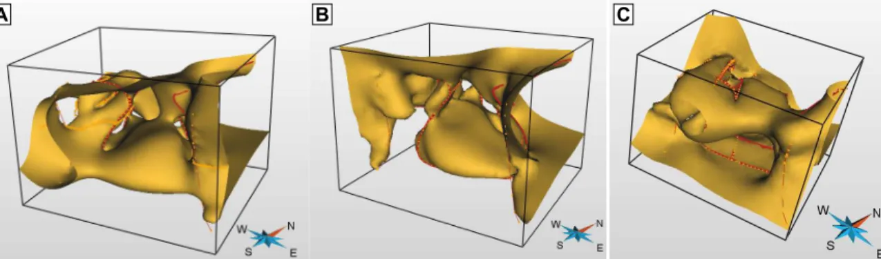
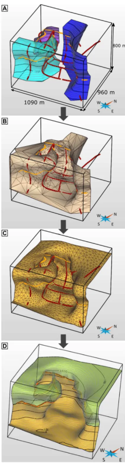
The indirect surface construction calls for projecting points onto the interpolated surface along specific directions, called shooting directions (Fig. 9C). The high sinuosity of the salt horizon and the pinched geometry of the central salt wall make this task challenging when a single initial surface is used, especially as its geometry is not yet definitive. This is why we decided to use a Divide and Conquer strategy that consists in creating surface patches, fitting them to data and merging them into the final surface (Fig. 9). In detail, we partitioned the input curves into simple domains, i.e. subsets for which projecting onto best fit plane is single-valued (Fig. 9A-B-C). Selecting slightly overlapping domains was important to ensure continuity between surface patches. Surface patches were fitted to data using the Discrete Smooth Interpolation (DSI) implemented in Gocad, which minimizes a weighted sum of the surface roughness and data misfit in the least square sense (Mallet, 1992, 2002) (Fig. 9D). Manual control and updating of the shooting directions was necessary during the interpolation steps. Then, we manually cut the overlapping parts (Fig. 9E and Fig. 10A). New surface parts were built by direct triangulation between opposite borders of the various surface patches to connect them coherently (Fig. 9F). The resulting connected components were merged to generate a single surface (Fig. 10B). Finally, some additional interpolation steps were performed to improve the data fit, and we manually refined and cleaned the surface mesh until obtaining the final salt surface (Fig. 10C-D).
Such an approach requires mastery of the modelling techniques but the resulting salt surface is directly the expression of interpretive concepts.
A Initial B
pointset
Partition of the data into 4 CDefinition of 4 initial
patches and shooting
D E
Overlapping area
FPatch linking
Figure 9: Principles of the Divide and Conquer strategy used to model the salt surface. To ease visualization, the steps are presented on a synthetic 2D case.
Modelling the mini-basin stratigraphy
The synclinal structure of the mini-basin, with steepened to vertical or overturned strata, allows the major part of the stratigraphic layers to outcrop. The traces of the strata on the topography are, however, discontinuous due to vegetation and surface processes (erosion and scree). The orientation measurements are also a crucial piece of information that has to be integrated into the modelling process. In such a case, implicit modelling methods have several advantages to coherently build stratigraphic series at once as compared to explicit methods (Caumon et al., 2013; Collon et al., 2015). Those methods consider geological interfaces as isovalues of a 3D scalar field f (x, y, z) and the outcropping stratigraphic lines correspond to level-set curves. These curves and the orientation data are used as constrain-ing data to interpolate a 3D scalar field on the whole volume of interest. Once this 3D scalar field has been computed, any stratigraphic surface can be explicitly constructed by extracting the corresponding isovalue surface. Consequently, despite the discontinuity of the stratigraphic lines on the topography, overlapping or leaking layers will be prevented inside the mini-basin. Here, we used a discrete interpolation scheme, meaning that the scalar field is defined by a piece-wise linear interpolation of the values stored at the vertices of a volumetric mesh. Thus, the scalar field computation required to first build a volumetric mesh.
Volumetric mesh generation The exposed gypsum wall that separates the eastern and western parts of the mini-basin is particularly pinched, with an observed width lower than 15 m in the thinnest part and a very abrupt closure (Fig. 11). This wall splits one single syncline in the north into two individualized synclines in the south. Stratigraphic
orienta-B C D 1090 m 960 m 800 m A
Figure 10: Modelling the salt surface: A - Surface patches are cut. B - Small surfaces are built by direct triangulation between adjacent borders to link the patches. Then all connected parts are merged to produce a single surface. C - The mesh is manually cleaned, and local refinement is performed to obtain a final smooth surface that fits the data. D -The final salt surface: the green part is located above the topography, while the yellow part is below.
tions are very different on both sides of the wall, demonstrating that it acts geometrically as a discontinuity. As a result, sedimentary layers must be interpolated independently on each side of this central diapir. In implicit modelling, integrating such a discontinuity can be handled by creating a tetrahedral mesh that is conformable to the discontinuity (Frank et al., 2007). Conformable means that tetrahedron facets that are located on one disconti-nuity surface are the same triangles as the one meshing the discontidisconti-nuity surface. The thin gypsum wall is, however, a complex area difficult to manage by meshing generators without making the number of mesh elements impractically large. Indeed, to compute an accurate enough interpolation of the scalar field, the tetrahedron edge length of this area should be less than 5 m, implying high memory and computational costs (this also motivated the choice of the explicit modelling for the salt surface). To simplify this area, we decided to create an equivalent model by replacing the pinched part by a discontinuity surface that can be assimilated to a weld. The salt surface was consistently truncated and closed to ensure a sealed contact of both surfaces as required by meshing generators (Fig. 11).
The volumetric mesh was then generated using the two-step method proposed by Botella et al. (2014) and implemented in the research library VorteXLib: (1) generation of the final vertices of the mesh from the boundary surfaces, (2) generation of a tetrahedral mesh constrained by the salt surface and the computed vertices using TetGen (Si, 2015). The final mesh is conformable to the salt surface and is made of around 4.5 million tetrahedra with an average edge length of 9 m (Fig. 12). For minimizing the memory cost while keeping a small tetrahedron edge length, the size of the initial zone of interest was reduced, particularly by removing the parts above the topography (Fig. 12).
Scalar field computation In the implicit modelling method we used, all constraints can be weighted according to their relative reliability. In other words, when two constraints act on the same point, the higher their weight W is, the more they influence the interpolated scalar field value. As for the salt surface modelling, our concern was to use all available outcrop data (stratigraphic lines and orientation measurements) and to limit as much as possible the addition of more interpretations. Thus, higher weights were attached to field data than to interpretive constraints. Five constraints with different weights W were suffi-cient and necessary to build a model of the mini-basin filling that fits our geological concepts (Fig. 13):
• The first three constraints impose directly the scalar field values:
– Each set of lines corresponding to the same interpreted strata defines a value of the scalar field (W = 100).
– These lines are completed by a few interpretive lines manually digitized to im-pose the shape above the topography (W = 50). Values are attached to them consistently with the previous set of lines.
– A surface located at 5 m from the external salt surface boundary accounts for the conformity of the sediment deposits right above the evaporitic substratum of the mini-basin (W = 1).
• The two last ones act indirectly by imposing the scalar field gradient: – Orientation measurements are used with a high weight W = 100.
– They are completed by a constant gradient constraint W = 20, necessary to smooth the scalar field away from the data points.
Figure 11: Equivalent model used for the volumetric mesh generation: we truncated the pinched part of the salt surface and replaced it by an equivalent surface of discontinuity. Surfaces are closed and mutually cut to ensure the sealed model required by mesh generators.
500 m 724 m 890 m 1090 m 960 m 800 m a) Initial zone of interest
b) Reduced zone of interest
c) Volumetric mesh
A
B
C
Figure 12: Volumetric mesh generation: we restrained the initial zone of interest (a) to limit the memory cost (b). We generated a volumetric mesh conformable to salt surface with the VorteXLib research library (Botella et al., 2014). Here, the mesh is partially sliced to propose an excavated view of the meshed mini-basin (in blue) and the diapiric body (in grey) (c).
with the constant norm imposed by the constant gradient constraint, i.e. they must evolve proportionally to their inter-distances. For that purpose, we used values proportional to the average apparent thickness between surfaces, ranging from 1 to 47 (Fig. 13-A and B). A value of 52 was also attached to the surface located at 5 m from the external salt surface boundary. On the external border, this surface was vertically extended upward to avoid a collapsing effect above the topographic surface, which the extrapolation of the upward tightening of the mini-basin would otherwise have induced (i.e., edge effect). It was also cut along the central salt wall to authorize discordant contacts between sediment layers and this halokinetic feature as observed on the field. The chosen weights give priority to field data while preserving global coherency far from them. Note that there is no relation between weights, which express our confidence in the data, and the scalar field values, which express the relative distance of the data from the zero isosurface. The resulting scalar field is shown on Figure 13-E. For visualization purposes, each surface corresponding to an isovalue imposed by an interpreted stratigraphic level has been extracted to produce the final model presented on Figure 14. Thanks to WebGL technology, the model can also be viewed in 3D at this url: http://ring.georessources.univ-lorraine.fr/model 3d html/Sivas.html.
DISCUSSION
The resulting geomodel of the Inceyol mini-basin fits all outcrop data while integrating previous geological interpretations. It reflects the ground observations at the chosen scale, but could not be validated as this would call for subsurface data, which are currently unavailable. Thus, the model complements quantitatively an existing interpretation of the data: it allows a three dimensional visualization of the complex and non intuitive geometry of such a salt-related structure. In itself, it is already an interesting achievement as such geometries are not easily reproduced with standard 3D geomodelling workflows and call for adapted strategies.
The various technical choices made to realize this model can still be discussed. The first one is the choice of the order of the modelling steps. In the field, the global coin-purse shape of the mini-basin is mostly deduced from the dip measurements of the outcropping strata, profile views in outcrop, analogy with neighbouring mini-basins and our conceptual analysis. In this concept-driven approach, the mini-basin infill has constrained the interpre-tive salt surface morphology. Based on that interpretation, the modelling workflow used the salt-sediment relation inversely: we decided to start modelling the salt surface to provide a geospatial constraint for the deepest layers of sediments. We chose that because modelling one surface is technically easier than modelling set of conformable surfaces, especially in areas of high curvature which are numerous in this case study. Furthermore, implicit meth-ods require the separation of the various sedimentary blocks to consistently interpolate the scalar field in independent areas. It is thus more suited to directly generate a mesh con-formable to the mini-basin boundaries (here the salt surface) with implicit methods. With explicit methods, indeed, we would create an approximate volumetric mesh with arbitrary vertical surfaces of discontinuity that might turn out to be misplaced at the end of the process.
A second point relates to the size of the represented structures. The central part of the study area is characterized by very tight features, particularly at the core of the syncline. With a syncline width smaller than 10 m, the average tetrahedron edge length of 9 m is
Scalar field B A C D E 1 60 890 m 500 m 724 m
Figure 13: Various constraints are used to compute the 3D scalar field (E): A - a scalar field value is affected to the stratigraphic lines observed on the topography; B - dip measurements impose a local scalar field gradient direction; C - additional interpretive lines imposes values above the topography; D - a surface located at 5 m from the salt boundary imposes the scalar field value on the external flanks of the mini-basin to ensure the deposit conformity to the salt layer on this area.
724 m 890 m 500 m Salt surface above the topography Salt surface below the topography A B C D
Figure 14: Resulting 3D model of the Inceyol mini-basin. The stratigraphic surfaces corre-spond to the extraction of the following isovalues of the scalar field : 1, 3, 4.5, 6, 10, 13.5, 18, 30, 36.5, 43, 47 and 50. A and B - Two different views; C and D - Two different slices in the 3D model. The model can also be viewed in 3D at this url: http://ring.georessources.univ-lorraine.fr/model 3d html/Sivas.html
not small enough to adequately describe the central horizon (corresponding to the value 1 of the scalar field) in the most strongly deformed areas of tight folds. Indeed, it supposes that the same value is observed twice on a single tetrahedron edge, which is not possible as values are carried by vertices and linearly interpolated along the edges. This limitation could be overcome with an adaptive mesh generation. It would require to use an additional surface, for example the isosurface corresponding to the value 10, to impose a refinement inside the central part (Botella et al., 2014) followed by re-interpolation.
Thirdly, in order to constrain the sediment layers to drape the salt horizon at the external part of the mini-basin, a controlling surface parallel to the salt surface has been created. This surface has been cut approximately 100 m above the mini-basin bottom to allow a discordant contact along the central salt wall edges, similarly to what was observed in the field. This depth choice is arbitrary but it allows us to fit the field observations and to reproduce the geometries of the conceptual cross sections. Somewhat equivalent solutions could have been obtained with a slightly upper or lower cut. Also, the sediment/salt contact along the central salt wall is the result of the smooth interpolation between the syncline data constraints on the younger strata and the conformable trend on the oldest layers. Thus, a tight fold of the strata is obtained against the central salt wall edges and the strata are conformable one to another. Salt-tectonics is, however, often characterized by more specific features like halokinetic sequences and their associated hook and wedge halokinetic sequence end-members (Giles and Rowan, 2012). Moreover, in the absence of clear data, the use of a constant gradient term is questionable, since it will tend to minimize the stratigraphic layer thickness variations. Being able to reproduce the tabular and/or tapered composite halokinetic sequences (Giles and Rowan, 2012; Hearon et al., 2014) and their associated end-members would be an interesting perspective of this work that would require further numerical developments. Indeed, in an implicit workflow, unconformity surfaces can be defined, but they are interpolated as independent conformable sequences (Calcagno et al., 2006; Durand-Riard et al., 2013) which can be limiting in sparse data settings.
The fourth point concerns the strategy chosen to build the salt surface. Even if the retained method was a patch-by-patch explicit approach, we think it could also be feasible with an implicit method. An adaptive tetrahedral mesh refined in the central area would be necessary to get the desired thin shape of the central gypsum wall; and it would require to add iteratively interpretive inputs until the scalar field computation would end in a satisfactory result. Our modelling choice was mainly guided by our own expertise and the possibility to directly and efficiently control the topology of the surface with the explicit approach. Thus, for deterministic modelling purposes, it is difficult at this point to make a general recommendation about one method versus another as it depends on the level of user expertise, data density and surface complexity. When dealing with uncertainty, implicit modelling should clearly be preferred, because it makes model perturbation much easier (Wellmann et al., 2010; Lindsay et al., 2012; Cherpeau and Caumon, 2015). In that case, it is always possible to build a base implicit representation from available data and some manually generated explicit surface. Moreover, the salt surface construction method based on patches was quite fast for an experienced modeller but more dedicated tools could be imagined to ease salt feature reproduction. Non Uniform Rational B-Splines (NURBS) have proven their ability to model complex tectonic structures (Sprague and de Kemp, 2005) and/or sedimentological structures like channels, clinoform and lobes (Ruiu et al., 2014, 2015). A similar approach could be developed for salt features.
Overall, this work produced only one possible 3D model of the complex architecture of the Inceyol mini-basin. High uncertainties are associated to its deep geometry and the validation of such a representation can still be debated. Exploring these uncertainties by incorporating small perturbations on the salt surface could be done in a similar way as proposed by Tertois and Mallet (2007) for fault networks. This method could also be used for local model update. But in the current state of the art, more important changes on the salt geometry would require manually rebuilding the complete model as automated model updating methods still have a limited capacity to address large-scale changes in input parameters. Perturbing the stratigraphy inside the mini-basin for a given salt geometry would probably be a more accessible goal in this framework based on implicit approach. Layer geometry could indeed be perturbed by adding realizations of a random field r(x, y, z) to the 3D scalar field f (x, y, z) (e.g., Caumon, 2010; Mallet, 2014; Cherpeau and Caumon, 2015). In all cases, additional data would be necessary to later reduce the uncertainties.
CONCLUSION
The Inceyol mini-basin constituted a real challenge for geomodelling: it has a specific geometry of an encased synclinal split southwards into two tight synclines by the rise of a central salt wall. Classical geomodelling tools or integrated strategies are not adapted to reproduce the convoluted salt surface shape in a context of very sparse data. In such concept-driven approach, we succeeded by using a careful patch by patch explicit surface modelling, completed by a manual mesh improvement step. The combined use of an implicit modelling approach, with specific weighted interpolation constraints, allowed us to generate a 3D model of the mini-basin sedimentary deposits consistent with the outcrop data and the interpretive cross-sections. With the inherent specificities of a case study, this work proves that building such complex models is feasible with the existing tools and a good expertise in the various geomodelling techniques
The resulting geomodel could constitute a good basis for supporting the quantitative interpretation of potential field data. Potential field data have indeed proven to help gaining insights into the geometrical definition of equivalent geological structures; but they need to be associated with 3D geomodels to be fully exploitable (e.g., Back´e et al., 2010; Gernigon et al., 2011; Lindsay et al., 2012). This work also raises a lot of interesting perspectives for dedicated numerical tool development, ranging from specific salt-related shape construction to halokinetic sequences reproduction, while better managing the associated uncertainties. In that aim, input data are proposed for download to constitute a reference case study.
ACKNOWLEDGEMENTS
A lot of persons contributed more or less directly to this case study. We warmly thank all of them :
• MSc students of the Nancy School of Geology (University of Lorraine), who measured the stratigraphic orientations during a field trip. They have made this an enjoyable adventure: Oc´eane Favreau, Ga´etan Fuss, Gabriel Godefroy, Marine Lerat, Antoine Mazuyer, Marion Parquer.
• Dr. Julien Charreau, Associate Professor in Nancy, who initiated the field trip by putting in touch our teams in Nancy and Pau. He also accompanied us in the field.
This work would not have emerged without him.
• Dr. Kaan Kavak, as well as Dr. Haluk Temiz, both Professors at Cumhuriyet University (Sivas, Turkey), who so warmly welcomed us in Sivas. They have made this field trip possible.
• Dr. Gautier Laurent, Research fellow in Nancy, who gave good ideas and suggestions for implicit modelling of salt surface.
• Total S.A. and ASGA, who funded the field trip.
• Dr A. Graham Leslie and Dr. E. de Kemp, who gave constructive remarks.
This work was performed in the frame of the RING project at Universit´e de Lorraine. We would like to thank the industrial and academic sponsors of the RING-Gocad Research Consortium managed by ASGA for their support. We also thank Paradigm for providing the SKUA-GOCAD software and API.
REFERENCES
Antoine, C., and G. Caumon, 2008, Rapid algorithm prototyping in Gocad using Python plugin.: Proc. 28th Gocad Meeting, 4.
Back´e, G., G. Baines, D. Giles, W. Preiss, and A. Alesci, 2010, Basin geometry and salt diapirs in the Flinders Ranges, South Australia: Insights gained from geologically-constrained modelling of potential field data: Marine and Petroleum Geology, 27, 650– 665.
Botella, A., B. L´evy, and G. Caumon, 2014, A new workflow for constrained tetrahedral mesh generation: application to structural models and hex-dominant meshing: Presented at the Proc. 34th Gocad Meeting, ASGA.
Calcagno, P., G. Courrioux, A. Guillen, D. Fitzgerald, and P. McInerney, 2006, How 3D im-plicit Geometric Modelling Helps To Understand Geology: The 3DGeoModeller Method-ology: Presented at the Proc. IAMG’06.
Callot, J.-P., C. Ribes, C. Kergaravat, C. Bonnel, H. Temiz, A. Poisson, B. Vrielynck, J.-f. Salel, and J.-c. Ringenbach, 2014, Salt Tectonics in the Sivas Basin (Turkey): Crossing salt walls and minibasins: Bulletin de la Soci´et´e g´eologique de France, 185, 33–42. Cater, J. M. L., S. S. Hanna, A. C. Ries, and P. Turner, 1991, Tertiary evolution of the
Sivas Basin, central Turkey: Tectonophysics, 195, 29–46.
Caumon, G., 2010, Towards stochastic time-varying geological modeling: Mathematical Geosciences, 42, 555–569.
Caumon, G., P. Collon-Drouaillet, C. Le Carlier de Veslud, S. Viseur, and J. Sausse, 2009, Surface-Based 3D Modeling of Geological Structures: Mathematical Geosciences, 41, 927–945.
Caumon, G., G. Gray, C. Antoine, and M.-O. Titeux, 2013, Three-Dimensional Implicit Stratigraphic Model Building From Remote Sensing Data on Tetrahedral Meshes: Theory and Application to a Regional Model of La Popa Basin, NE Mexico: IEEE Transactions on Geoscience and Remote Sensing, 51, 1613–1621.
Cherpeau, N., and G. Caumon, 2015, Stochastic structural modelling in sparse data situa-tions: Petroleum Geoscience, 21, 233–247.
Collon, P., W. Steckiewicz-laurent, J. Pellerin, L. Gautier, G. Caumon, G. Reichart, and L. Vaute, 2015, 3D geomodelling combining implicit surfaces and Voronoi-based remeshing : A case study in the Lorraine Coal Basin (France): Computers & Geosciences, 77, 29–43. Durand-Riard, P., C. Guzofski, G. Caumon, and M.-O. Titeux, 2013, Handling natural complexity in three-dimensional geomechanical restoration, with application to the recent evolution of the outer fold and thrust belt, deep-water Niger Delta: AAPG bulletin, 97, 87–102.
Fossen, H., 2010, Structural Geology: Cambridge University Press.
Frank, T., A.-L. Tertois, and J.-L. Mallet, 2007, 3D-reconstruction of complex geological interfaces from irregularly distributed and noisy point data: Computers and Geosciences, 33, 932–943.
Gernigon, L., M. Br¨onner, C. Fichler, L. Løvas, L. Marello, and O. Olesen, 2011, Magnetic expression of salt diapir-related structures in the Nordkapp Basin, western Barents Sea: Geology, 39, 135–138.
Giles, K. A., and T. F. Lawton, 2002, Halokinetic sequence stratigraphy adjacent to the El Papalote diapir, northeastern Mexico: AAPG bulletin, 86, 823–840.
Giles, K. A., and M. G. Rowan, 2012, Concepts in halokinetic-sequence deformation and stratigraphy: Geological Society, London, Special Publications, 363, 7–31.
Guezou, J.-C., H. Temiz, A. Poisson, and H. G¨ursoy, 1996, Tectonics of the Sivas basin: The Neogene record of the Anatolian accretion along the inner Tauric suture: International Geology Review, 38, 901–925.
G¨undogan, I., M. ¨Onal, and T. Dep¸ci, 2005, Sedimentology, petrography and diagenesis of Eocene–Oligocene evaporites: the Tuzhisar Formation, SW Sivas Basin, Turkey: Journal of Asian Earth Sciences, 25, 791–803.
Haecker, M. A., 1992, Convergent gridding: a new approach to surface reconstruction: Geobyte, 7, 48–53.
Hearon, T. E., M. G. Rowan, K. A. Giles, and W. H. Hart, 2014, Halokinetic deformation adjacent to the deepwater Auger diapir , Garden Banks 470 , northern Gulf of Mexico : Testing the applicability of an outcrop-based model using subsurface data: Interpretation, 2, SM57–SM76.
Hudec, M. R., and M. P. A. Jackson, 2007, Terra infirma: understanding salt tectonics: Earth-Science Reviews, 82, 1–28.
Jackson, C. A.-L., C. R. Rodriguez, A. Rotevatn, and R. E. Bell, 2014, Geological and geophysical expression of a primary salt weld: An example from the Santos Basin, Brazil: Interpretation, 2, SM77–SM89.
Jackson, M. P. A., and J. C. Harrison, 2006, An allochthonous salt canopy on Axel Heiberg Island, Sverdrup Basin, Arctic Canada: Geology, 34, 1045–1048.
Jahani, S., J.-P. Callot, J. Letouzey, and D. de Lamotte, 2009, The eastern termination of the Zagros Fold-and-Thrust Belt, Iran: Structures, evolution, and relationships between salt plugs, folding, and faulting: Tectonics, 28, 1–22.
Kaven, J., R. Mazzeo, and D. Pollard, 2009, Constraining surface interpolations using elastic plate bending solutions with applications to geologic folding: Mathematical Geosciences, 41, 1–14.
Kergaravat, C., 2016, Dynamique de formation et de d´eformation de mini-bassins en con-texte compressif : Approche terrain, implications structurales multi-´echelles et r´eservoirs (exemple du bassin de Sivas, Turquie): PhD thesis, Universit´e de Pau et des Pays de l’Adour, Pau, France.
Kurtman, F., 1973, Geologic and tectonic structure of the Sivas- Hafik-Zara and Imranli Region: Bulletin Mineral Research and Exploration (Ankara, Turkey), 80, 1–32.
Lindsay, M. D., L. Aill`eres, M. W. Jessell, E. A. de Kemp, and P. G. Betts, 2012, Locat-ing and quantifyLocat-ing geological uncertainty in three-dimensional models: analysis of the Gippsland Basin, southeastern Australia: Tectonophysics, 546-547, 10–27.
Mallet, J.-L., 1992, Discrete Smooth Interpolation: Computer-Aided Design, 24, 263–270. ——–, 2002, Geomodeling: Oxford University Press, New York, NY. Applied Geostatistics. ——–, 2014, Elements of mathematical sedimentary geology: The GeoChron model: EAGE. Pichat, A., G. Hoareau, J.-M. Rouchy, C. Ribes, C. Kergaravat, J.-P. Callot, and J.-C. Ringenbach, 2015, Deposition and evolution of the Sivas basin evaporites (Turkey): Geo-physical Research Abstract, EGU General Assembly 2015, 9091.
Poisson, A., and J. C. Guezou, 1996, Tectonic Setting and Evolution of the Sivas Basin, Central Anatolia, Turkey: International Geology Review, 38, 838–853.
Ribes, C., C. Kergaravat, C. Bonnel, P. Crumeyrolle, J.-P. Callot, A. Poisson, H. Temiz, and J.-C. Ringenbach, 2015, Fluvial sedimentation in a salt-controlled mini-basin: stratal patterns and facies assemblages, Sivas Basin, Turkey: Sedimentology, 62, 1513–1545. Ribes, C., C. Kergaravat, P. Crumeyrolle, M. Lopez, C. Bonnel, A. Poisson, K. S. Kavak,
J.-P. Callot, and J.-C. Ringenbach, 2016, Factors controlling stratal pattern and facies dis-tribution of fluvio-lacustrine sedimentation in the Sivas mini-basins, Oligocene (Turkey):
Basin Research, –, 1–26.
Ringenbach, J.-C., J.-F. Salel, C. Kergaravat, C. Ribes, C. Bonnel, and J.-P. Callot, 2013, Salt tectonics in the Sivas Basin , Turkey : outstanding seismic analogues from outcrops: First Break, 31, 93–101.
Rowan, M. G., T. E. Hearon, F. J. Peel, S. Stewart, O. Ferrer, J. C. Fiduk, S. Holdaway, W. U. Mohriak, V. Mount, D. G. Quirk, and T. Seeley, 2014, Introduction to special section : Salt tectonics and interpretation: Interpretation, 2, SMi.
Rowan, M. G., and B. C. Vendeville, 2006, Foldbelts with early salt withdrawal and di-apirism: physical model and examples from the northern Gulf of Mexico and the Flinders Ranges, Australia: Marine and Petroleum Geology, 23, 871–891.
Ruiu, J., G. Caumon, and S. Viseur, 2015, Semiautomatic interpretation of 3D sedimen-tological structures on geologic images: An object-based approach: Interpretation, 3, SX63—-SX74.
Ruiu, J., G. Caumon, S. Viseur, and C. Antoine, 2014, Modeling Channel Forms Using a Boundary Representation Based on Non-uniform Rational B-Splines, in Mathematics of Planet Earth: Springer, 581–584.
Si, H., 2015, TetGen, a Delaunay-Based Quality Tetrahedral Mesh Generator: ACM Trans-actions on Mathematical Software, 41, 1–36.
Sprague, K. B., and E. A. de Kemp, 2005, Interpretive tools for 3-D structural geological modelling part II: Surface design from sparse spatial data: GeoInformatica, 9, 5–32. Tertois, a. L., and J. L. Mallet, 2007, Editing faults within tetrahedral volume models in
real time: Geological Society, London, Special Publications, 292, 89–101.
Trocm´e, V., E. Albouy, J.-P. Callot, J. Letouzey, N. Rolland, H. Goodarzi, and S. Ja-hani, 2011, 3D structural modelling of the southern Zagros fold-and-thrust belt diapiric province: Geological Magazine, 148, 879–900.
Vendeville, B., H. Ge, and M. P. A. Jackson, 1995, Scale models of salt tectonics during basement-involved extension: Petroleum Geoscience, 1, 179–183.
Wellmann, J. F., F. G. Horowitz, E. Schill, and K. Regenauer-Lieb, 2010, Towards incor-porating uncertainty of structural data in 3D geological inversion: Tectonophysics, 490, 141–151.