Virtual Compton Scattering and the Generalized Polarizabilities of the Proton at Q^2=0.92 and 1.76 GeV^2

arXiv:1205.3387v2 [nucl-ex] 28 Jun 2012

Q

=0.92 and 1.76 GeV

H. Fonvieille∗_,1 _{G. Laveissi`ere,}1_{N. Degrande,}2 _{S. Jaminion,}1 _{C. Jutier,}1, 3 _{L. Todor,}3 _{R. Di Salvo,}1 _{L. Van}

Hoorebeke,2 _{L.C. Alexa,}4 _{B.D. Anderson,}5_{K.A. Aniol,}6 _{K. Arundell,}7 _{G. Audit,}8 _{L. Auerbach,}9 _{F.T. Baker,}10

M. Baylac,8_{J. Berthot}†_,1 _{P.Y. Bertin,}1 _{W. Bertozzi,}11 _{L. Bimbot,}12 _{W.U. Boeglin,}13 _{E.J. Brash,}4 _{V. Breton,}1

H. Breuer,14 _{E. Burtin,}8 _{J.R. Calarco,}15_{L.S. Cardman,}16 _{C. Cavata,}8_{C.-C. Chang,}14_{J.-P. Chen,}16_{E. Chudakov,}16

E. Cisbani,17 _{D.S. Dale,}18_{C.W. de Jager,}16_{R. De Leo,}19 _{A. Deur,}1, 16 _{N. d’Hose,}8 _{G.E. Dodge,}3 _{J.J. Domingo,}16

L. Elouadrhiri,16 _{M.B. Epstein,}6 _{L.A. Ewell,}14 _{J.M. Finn}†_,7 _{K.G. Fissum,}11_{G. Fournier,}8_{B. Frois,}8 _{S. Frullani,}17

C. Furget,20 _{H. Gao,}11_{J. Gao,}11 _{F. Garibaldi,}17_{A. Gasparian,}21, 18 _{S. Gilad,}11 _{R. Gilman,}22, 16 _{A. Glamazdin,}23

C. Glashausser,22 _{J. Gomez,}16 _{V. Gorbenko,}23_{P. Grenier,}1 _{P.A.M. Guichon,}8 _{J.O. Hansen,}16 _{R. Holmes,}24

M. Holtrop,15 _{C. Howell,}25 _{G.M. Huber,}4 _{C.E. Hyde,}3, 1 _{S. Incerti,}9 _{M. Iodice,}17 _{J. Jardillier,}8 _{M.K. Jones,}7

W. Kahl,24 _{S. Kato,}26 _{A.T. Katramatou,}5_{J.J. Kelly}†_,14 _{S. Kerhoas,}8_{A. Ketikyan,}27 _{M. Khayat,}5 _{K. Kino,}28

S. Kox,20 _{L.H. Kramer,}13 _{K.S. Kumar,}29 _{G. Kumbartzki,}22_{M. Kuss,}16 _{A. Leone,}30 _{J.J. LeRose,}16 _{M. Liang,}16

R.A. Lindgren,31 _{N. Liyanage,}11_{G.J. Lolos,}4_{R.W. Lourie,}32 _{R. Madey,}5 _{K. Maeda,}28_{S. Malov,}22 _{D.M. Manley,}5

C. Marchand,8 _{D. Marchand,}8_{D.J. Margaziotis,}6_{P. Markowitz,}13_{J. Marroncle,}8_{J. Martino,}8 _{K. McCormick,}3

J. McIntyre,22 S. Mehrabyan,27 F. Merchez,20 Z.E. Meziani,9 R. Michaels,16 G.W. Miller,29J.Y. Mougey,20 S.K. Nanda,16 _{D. Neyret,}8 _{E.A.J.M. Offermann,}16 _{Z. Papandreou,}4_{B. Pasquini,}33 _{C.F. Perdrisat,}7_{R. Perrino,}30

G.G. Petratos,5_{S. Platchkov,}8 _{R. Pomatsalyuk,}23_{D.L. Prout,}5_{V.A. Punjabi,}34_{T. Pussieux,}8 _{G. Qu´emen´er,}1, 7

R.D. Ransome,22O. Ravel,1 J.S. Real,20F. Renard,8 Y. Roblin,1 D. Rowntree,11 G. Rutledge,7 P.M. Rutt,22 A. Saha†_,16 _{T. Saito,}28 _{A.J. Sarty,}35_{A. Serdarevic,}4, 16 _{T. Smith,}15 _{G. Smirnov,}1 _{K. Soldi,}36 _{P. Sorokin,}23

P.A. Souder,24 _{R. Suleiman,}11 _{J.A. Templon,}10 _{T. Terasawa,}28 _{R. Tieulent,}20 _{E. Tomasi-Gustaffson,}8

H. Tsubota,28 H. Ueno,26 P.E. Ulmer,3 G.M. Urciuoli,17 M. Vanderhaeghen,37R.L.J. Van der Meer,16, 4 R. Van De Vyver,2 _{P. Vernin,}8 _{B. Vlahovic,}16, 36 _{H. Voskanyan,}27_{E. Voutier,}20 _{J.W. Watson,}5_{L.B. Weinstein,}3

K. Wijesooriya,7 _{R. Wilson,}38_{B.B. Wojtsekhowski,}16_{D.G. Zainea,}4 _{W-M. Zhang,}5 _{J. Zhao,}11_{and Z.-L. Zhou}11

(The Jefferson Lab Hall A Collaboration)

1_{Clermont-Universit´e, UBP, CNRS-IN2P3, LPC, BP 10448, F-63000 Clermont-Ferrand, France} 2_{Department of Physics and Astronomy, Ghent University, B-9000 Ghent, Belgium}

3_{Old Dominion University, Norfolk, VA 23529} 4_{University of Regina, Regina, SK S4S OA2, Canada}

5_{Kent State University, Kent OH 44242}

6_{California State University, Los Angeles, Los Angeles, CA 90032} 7_{College of William and Mary, Williamsburg, VA 23187} 8_{CEA IRFU/SPhN Saclay, F-91191 Gif-sur-Yvette, France}

9_{Temple University, Philadelphia, PA 19122} 10_{University of Georgia, Athens, GA 30602}

11_{Massachusetts Institute of Technology, Cambridge, MA 02139}

12_{Institut de Physique Nucl´eaire (UMR 8608), CNRS/IN2P3 - Universit´e Paris-Sud, F-91406 Orsay Cedex, France} 13_{Florida International University, Miami, FL 33199}

14_{University of Maryland, College Park, MD 20742} 15_{University of New Hampshire, Durham, NH 03824}

16_{Thomas Jefferson National Accelerator Facility, Newport News, VA 23606} 17_{INFN, Sezione Sanit`a and Istituto Superiore di Sanit`a, 00161 Rome, Italy}

18_{University of Kentucky, Lexington, KY 40506}

19_{INFN, Sezione di Bari and University of Bari, 70126 Bari, Italy}

20_{LPSC Grenoble, Universite Joseph Fourier, CNRS/IN2P3, INP, F-38026 Grenoble, France} 21_{Hampton University, Hampton, VA 23668}

22_{Rutgers, The State University of New Jersey, Piscataway, NJ 08855} 23_{Kharkov Institute of Physics and Technology, Kharkov 61108, Ukraine}

24_{Syracuse University, Syracuse, NY 13244} 25_{Duke University, Durham, NC 27706} 26_{Yamagata University, Yamagata 990, Japan} 27_{Yerevan Physics Institute, Yerevan 375036, Armenia}

28_{Tohoku University, Sendai 980, Japan} 29_{Princeton University, Princeton, NJ 08544} 30_{INFN, Sezione di Lecce, 73100 Lecce, Italy} 31_{University of Virginia, Charlottesville, VA 22901}

33_{Dipartimento di Fisica, Universit`a degli Studi di Pavia, and INFN, Sezione di Pavia, Italy} 34_{Norfolk State University, Norfolk, VA 23504}

35_{Florida State University, Tallahassee, FL 32306} 36_{North Carolina Central University, Durham, NC 27707}

37_{Institut fuer Kernphysik, Johannes Gutenberg University, D-55099 Mainz, Germany} 38_{Harvard University, Cambridge, MA 02138}

Virtual Compton Scattering (VCS) on the proton has been studied at Jefferson Lab using the exclusive photon electroproduction reaction ep → epγ. This paper gives a detailed account of the analysis which has led to the determination of the structure functions PLL− PT T/ǫ and PLT, and

the electric and magnetic generalized polarizabilities (GPs) αE(Q2) and βM(Q2) at values of the

four-momentum transfer squared Q2= 0.92 and 1.76 GeV2. These data, together with the results of VCS experiments at lower momenta, help building a coherent picture of the electric and magnetic GPs of the proton over the full measured Q2_{-range, and point to their non-trivial behavior.}

PACS numbers: 13.60.-r,13.60.Fz

I. INTRODUCTION

The nucleon is a composite object, and understand-ing its structure is the subject of intensive efforts. Its electromagnetic structure is cleanly probed by real and virtual photons. Real Compton scattering (RCS) at low energy gives access to the nucleon polarizabilities, which describe how the charge, magnetization and spin densi-ties in the nucleon are deformed when the particle is sub-jected to an external quasi-static electromagnetic field.

Virtual Compton scattering (VCS) γ∗_{N → γN gives}

access to the generalized polarizabilities (GPs). Being de-pendent on the photon virtuality Q2_{, these observables}

parametrize the local polarizability response of the sys-tem, i.e. they give information on the density of polariza-tion inside the nucleon. Experimental informapolariza-tion on the GPs is obtained through the reaction of exclusive photon electroproduction. Several dedicated experiments on the proton:

e p → e p γ (1)

have been performed at various Q2_{and in the low-energy}

regime. This includes the near-threshold region, where the center-of-mass energy W of the (γp) system is be-low the one-pion threshold (W < (mp+ mπ0), where m_p

and mπ0 are the proton and pion masses), and up to the

∆(1232) resonance region. Process (1) has been stud-ied experimentally at MAMI [1–4], the Thomas Jeffer-son National Accelerator Facility (JLab) [5, 6] and MIT-Bates [7, 8].

The results of the near-threshold VCS data analysis of the JLab VCS experiment E93-050, i.e. the struc-ture functions PLL− PT T/ǫ and PLT, and the electric

and magnetic GPs αE and βM at Q2= 0.92 and 1.76

GeV2_{, have been published elsewhere [5]. However,}

anal-ysis details and cross section data were not given. This is the aim of the present paper, which is organized as

∗_{corresponding author, helene@clermont.in2p3.fr} †_deceased

follows. After recalling briefly the theoretical concepts in section II, the experimental setup is described in sec-tion III. Secsec-tion IV reports about data analysis, including event reconstruction, acceptance calculation and cross section determination. Section V presents the measured cross section, the physics results deduced from the vari-ous analyses, and a discussion. A short conclusion ends the paper in section VI.

II. THEORETICAL CONCEPTS AND TOOLS

FOR EXPERIMENTS

This section summarizes the theoretical concepts un-derlying the measurements of VCS at low energy: the GPs, the structure functions, and the principles of mea-surement. For details, we refer to review papers: [9–11] (theory) and [12–16] (experiments).

A. Generalized polarizabilities

Polarizabilities are fundamental characteristics of any composite system, from hadrons to atoms and

molecules. They describe how the system

re-sponds to an external quasi-static electromagnetic

field. Real Compton Scattering (RCS) yields

for the static polarizabilities of the proton [17]: αE (electric) = (12.1 ±0.3stat∓ 0.4syst) · 10−4f m3

βM (magnetic) = (1.6 ±0.4stat± 0.4syst) · 10−4f m3.

These values are much smaller than the particle’s volume and indicate that the proton is a very stiff object, due to the strong binding between its constituents.

The formalism of VCS on the nucleon was early ex-plored in [18] and the concept of generalized polariz-abilities was first introduced in [19] for nuclei. The nu-cleon case was established within a Low Energy Theorem (LET), first applied to VCS by P. Guichon et al. in [20]. This development paved the way to new experimental in-vestigations: it became possible to explore the spatial dis-tribution of the nucleon’s polarizability response, which is in essence the physical meaning of the GPs (see e.g.

[21, 22]).

Photon electroproduction accesses VCS via the ampli-tude decomposition shown in Fig. 1: Tepγ _{= T}BH ₊

TV CSBorn _{+ T}V CSN onBorn_{, where BH stands for the}

Bethe-Heitler process. Formally the GPs are obtained from the multipole decomposition of the Non-Born am-plitude TV CSN onBorn _{taken in the “static field” limit}

q′

c.m. → 0, where q′c.m. is the momentum of the final

real photon in the γp center-of-mass (noted CM here-after). The GPs are functions of qc.m., the momentum of

the virtual photon in the CM, or equivalently the photon virtuality Q2 _{(see Appendix A for more details). After}

the work of Drechsel et al. [23, 24], six independent GPs remain at lowest order. Their standard choice is given in Table I, where they are indexed by the EM transitions in-volved in the Compton process. Since this paper mainly focuses on the electric and magnetic GPs, i.e. the two scalar ones (or spin-independent, or non spin-flip, S=0; see Table I), we recall their definition:

αE(Q2) = −P(L1,L1)0(Q2) · (e 2 4π q 3 2) , βM(Q2) = −P(M1,M1)0(Q2) · (e 2 4π q 3 8) .

These GPs coincide in the limit Q2_{→ 0 with the usual}

static RCS polarizabilities αE and βM introduced above. TABLE I: The standard choice for the nucleon GPs. In the notation of the first column, ρ(ρ′_{) refers to the magnetic (1)}

or longitudinal (0) nature of the initial (final) photon, L(L′₎

represents the angular momentum of the initial (final) photon, and S differentiates between the spin-flip (S = 1) and non spin-flip (S = 0) character of the transition at the nucleon side. The multipole notation in the second column uses the magnetic (M) and longitudinal (L) multipoles. The six listed GPs correspond to the lowest possible order in q′

c.m., i.e. a

dipole final transition (L′ _{= 1). The third column gives the}

correspondence in the RCS limit (Q2_{→ 0 or q}

c.m.→ 0). P(ρ′L′_,ρL)S (qc.m.) P(f,i)S(qc.m.) RCS limit P(01,01)0 _P(L1,L1)0 ₋4π e2 p₂ 3 αE P(11,11)0 _P(M 1,M 1)0 ₋4π e2 p8 3 βM P(01,01)1 _P(L1,L1)1 ₀ P(11,11)1 _P(M 1,M 1)1 ₀ P(01,12)1 _P(L1,M 2)1 ₋4π e2 √ 2 3 γ3 P(11,02)1 P(M 1,L2)1 −4π_e2 2√2 3√3(γ2+ γ4)

B. Theoretical models and predictions There are a number of theoretical models which de-scribe and calculate the GPs of the nucleon. They include: heavy baryon chiral perturbation theory (HBChPT) [25–27], non-relativistic quark constituent models [20, 28–30], dispersion relations [10, 31, 32], linear-σ model [33, 34], effective Lagrangian model [35],

Skyrme model [36], the covariant framework of ref.[37], or more recent works regarding GPs redefinition [38], man-ifestly Lorentz-invariant baryon ChPT[39], or light-front interpretation of GPs [22].

One of the main physical interests of GPs is that they can be sensitive in a specific way to the various physical degrees of freedom, e.g. the nucleon core and the meson cloud. Thus their knowledge can bring novel information about nucleon structure. The electric GP is usually pre-dicted to have a smooth fall-off with Q2. The magnetic GP has two contributions, of paramagnetic and diamag-netic origin; they nearly cancel, making the total magni-tude small. As will be shown in section V C, the available data more or less confirm these trends. A synthesis of di-verse GP predictions for the proton is presented in [30].

p a)Bethe-Heitler b)VCS Born e e’ p p’ γ c)VCS Non-Born p p , N ,∗ ∆ ...

FIG. 1: (Color online) Feynman graphs of photon electropro-duction.

C. The Low Energy Theorem and the structure functions

The LET established in [20] is a major tool for ana-lyzing VCS experiments. The LET describes the photon electroproduction cross section below the pion threshold in terms of GPs. The (unpolarized) ep → epγ cross sec-tion at small q′

c.m. is written as:

d5σ = d5σBH+Born + q′c.m.· φ · Ψ0 + O(qc.m.′2 ) . (1)

The notation d5_{σ stands for d}5_σ/dk′

elabdΩ′elabdΩC.M.

where k′

elab is the scattered electron momentum, dΩ′elab

its solid angle and dΩγc.m. the solid angle of the

outgo-ing photon (or proton) in the CM; φ is a phase-space factor. The (BH+Born) cross section is known and cal-culable, with the proton electromagnetic form factors Gp_E and Gp_M as inputs. The Ψ0 term represents the leading

polarizability effect. It is given by: Ψ0= v1· (PLL−

1

ǫPT T) + v2· PLT , (2) where PLL, PT T and PLT are three unknown structure

functions, containing the GPs. ǫ is the usual virtual photon polarization parameter and v1, v2 are

kinemat-ical coefficients depending on (qc.m., ǫ, θc.m., ϕ) (see [9]

to point in the z-direction. The Compton angles are the polar angle θc.m. of the outgoing photon in the CM and

the azimuthal angle ϕ between the leptonic and hadronic planes; see Fig. 2.

The expressions of the structure functions useful to the present analysis are summarized here:

PLL = 4mp αem · G p E(Q2) · αE(Q2) , PT T = [PT T spin] , PLT = −2m_α p em q q2 c.m. Q2 · G p E(Q 2_{) · β} M(Q2) + [PLT spin] , (3)

where αem is the fine structure constant. The terms in

square brackets are the spin part of the structure func-tions (i.e. containing only spin GPs) and the other terms are the scalar parts. The important point is that the electric and magnetic GPs enter only in PLL and in the

scalar part of PLT, respectively.

In an unpolarized experiment at fixed Q2 _{and fixed}

ǫ, such as ours, only two observables can be determined using the LET: PLL − PT T/ǫ and PLT, i.e. only two

specific combinations of GPs. To further disentangle the GPs, one can in principle make an ǫ-separation of PLL

and PT T (although difficult to achieve), and in order to

extract all individual GPs one has to resort to double po-larization [40]. Here we perform a LET, or LEX (for Low-energy EXpansion) analysis in the following way: the two structure functions PLL− PT T/ǫ and PLT are extracted

by a linear fit of the difference d5_σexp_{− d}5_σBH+Born_,

based on eqs.(1) and (2), and assuming the validity of the truncation of the expansion to O(q′2

c.m.). Then, to further

isolate the scalar part in these structure functions, i.e. to access αE(Q2) and βM(Q2), a model input is required,

since the spin part is not known experimentally.

p

p’

ϕ

θ

γ

’

e’

e

γ∗

FIG. 2: (Color online) (ep → epγ) kinematics; four-momentum vectors notation and Compton angles (θc.m., ϕ)

in the γp center-of-mass.

D. The Dispersion Relations model

The Dispersion Relation (DR) approach is the second tool for analyzing VCS experiments. It is of particular importance in our case, so we briefly review its properties in this section. The DR formalism was developed by B.Pasquini et al. [10, 32] for RCS and VCS. Contrary to the LET which is limited to the energy region below the pion threshold, the DR formalism is also valid in the energy region up to the ∆(1232) resonance -an advantage fully exploited in our experiment.

The Compton tensor is parametrized through twelve invariant amplitudes Fi(i = 1, · · · , 12). The GPs are

ex-pressed in terms of the non-Born part FN B

i of these

am-plitudes at the point t = −Q2_{, ν = (s − u)/4m} p = 0,

where s, t, u are the Mandelstam variables of the Comp-ton scattering. The FN B

i amplitudes, except for two of

them, fulfill unsubtracted dispersion relations. When working in the energy region up to the ∆(1232), these s-channel integrals are considered to be saturated by the πN intermediate states. In practice, the calculation uses the MAID pion photo- and electroproduction multipoles [41], which include both resonant and non-resonant pro-duction mechanisms.

The amplitudes F1and F5have an unconstrained part,

corresponding to asymptotic contributions and dispersive contributions beyond πN . For F5 this part is dominated

by the t-channel π0 _{exchange; with this input, all four}

spin GPs are fixed in the model. For F1, a main feature

is that in the limit (t = −Q2_{, ν = 0) its non-Born part is}

proportional to the magnetic GP. The unconstrained part of FN B

1 is estimated by an energy-independent function

noted ∆β, and phenomenologically associated with the t-channel σ-meson exchange. This leads to the expression: βM(Q2) = βπN(Q2) + ∆β(Q2) , (4)

where βπN_{is the dispersive contribution calculated using}

MAID multipoles. The ∆β term is parametrized by a dipole form:

∆β = [β

exp_{− β}πN_] Q2₌₀

(1 + Q2/Λ2_β)2 . (5)

An unconstrained part is considered also for a third am-plitude, F2. Since in the limit (t = −Q2, ν = 0) the

non-Born part of F2 is proportional to the sum (αE+ βM),

one finally ends with a decomposition similar to eq.(5) for the electric GP itself:

αE(Q2) = απN(Q2) + ∆α(Q2) , with ∆α = [α exp_{− α}πN_] Q2₌₀ (1 + Q2_/Λ2 α)2 . (6)

The implication for experiments is that in the DR model the two scalar GPs are not fixed. They depend on the free parameters Λα and Λβ (dipole masses), which

can be fitted from data. It must be noted that the choice of a dipole form in eqs.(5) and (6) is arbitrary: Λα and

Λβ only play the role of intermediate quantities in

or-der to extract VCS observables, with minimal model-dependence. These parameters are not imposed to be constant with Q2_{. Our experimental DR analysis}

con-sists in adjusting Λα and Λβ by a fit to the measured

cross section, separately in our two Q2_{-ranges. Then,}

in each Q2-range the model is entirely constrained; it provides all VCS observables, at a given value of Q2

rep-resentative of the range: the scalar GPs as well as the structure functions, in particular PLL− PT T/ǫ and PLT.

III. THE EXPERIMENT

The photon electroproduction cross section is small and requires a high-performance equipment to be mea-sured with accuracy. To ensure the exclusivity of the reaction, one must detect at least two of the three par-ticles in the final state. The chosen technique is to per-form electron scattering at high luminosity on a dense proton target, and detect in coincidence the two outgo-ing charged particles in magnetic spectrometers of high resolution and small solid angle. These devices ensure a clean detection and a good identification of process (1). Section III describes how the experiment was designed and realized using the CEBAF electron beam and the JLab Hall A equipment.

A. Apparatus

Since the Hall was in its commissioning phase at the time of the data taking for this experiment (1998), not all devices were fully operational and the minimal num-ber of detectors were used. However the experiment fully exploited the main capabilities of the accelerator and the basic Hall equipment: 100% duty cycle, high resolution spectrometers, high luminosities. The Hall A instrumen-tation is described extensively in ref. [42] and in several thesis works related to the experiment [43–47]. Only a short overview is given here, and some specific details are given in the subsections.

The continuous electron beam at 4 GeV energy (un-polarized) was sent to a 15 cm long liquid hydrogen tar-get. The two High Resolution Spectrometers, noted here HRS-E and HRS-H, were used to detect in coincidence an outgoing electron and proton, respectively. After exit-ing the target region the particles in each HRS encounter successively: the entrance collimator of 6 msr, the mag-netic system (QQDQ), and the detector package. The latter consisted of a set of four vertical drift chambers (VDC), followed by two scintillator planes S1 and S2. It was complemented in the HRS-E by a Cerenkov detec-tor and a shower counter, and in the HRS-H by a focal plane polarimeter. The VDCs provided particle tracking in the focal plane. The scintillators were the main trig-ger elements. They provided the timing information in each spectrometer and allowed to form the coincidence trigger.

B. Kinematical settings and data taking Data were taken in two different Q2_{-ranges, near 0.9}

and 1.8 GeV2_{. The corresponding data sets are labelled}

I and II, respectively. At Q2= 0.9 GeV2dedicated data were taken in the region of the nucleon resonances [6]. This leads us to split data set I into two independent subsets, I-a and I-b, according to the W -range. Figure 3

displays the various domains covered in W , or equiva-lently q′

c.m.. Data sets I-a and II have events essentially

below the pion threshold, while data set I-b is more fo-cused on the ∆(1232) resonance region and above. For the analyses presented here, emphasis will be put on data sets I-a and II. For data set I-b, details can be found already in [6], in which a nucleon resonance study was performed up to W = 2 GeV. Here, the lowest-W part of data set I-b is analyzed in terms of GPs. Table II summarizes our notations.

TABLE II: The various data sets of the experiment. Columns 2 and 3 give the ranges in Q2 _{and W covered by the}

exper-iment. The fixed value of Q2 chosen in the analyses is 0.92 GeV2 _{(resp. 1.76 GeV}2_{) for data sets I-a and I-b (resp. II).}

Columns 4 and 5 give the W -range used in the LEX and DR analyses.

data Q2-range W -range W -range W -range

set (GeV2_{) (GeV) LEX (GeV) DR (GeV)}

I-a [0.85, 1.15] [0.94, 1.25] [0.94, 1.07] [0.94, 1.25] I-b [0.85, 1.15] [1.00, 2.00] —– [1.00, 1.28] II [1.60, 2.10] [0.94, 1.25] [0.94, 1.07] [0.94, 1.25]

0 2000

counts per 8 MeV/c

data set I-a (<Q2> = 0.92 GeV2)

0 2000

0 500

data set I-b (<Q2> = 0.92 GeV2)

0 500

0 2000

0 100 200 300 400 500 600 700 800

data set II (<Q2> = 1.76 GeV2)

0 2000 0 100 200 300 400 500 600 700 800 q , (MeV/c) c.m. 1.0 1.2 1.4 1.6 1.8 2.0 W (GeV) (c) (b) (a)

FIG. 3: (Color online) The range in q′

c.m., or W , covered by

the various data sets for the ep → epγ events. The vertical lines show the upper limit applied in the analyses: the pion threshold (dotted line at W = 1.073 GeV) for the LEX anal-yses and W = 1.28 GeV (dashed line) for the DR analanal-yses. W and q′

c.m.are related by W = q′c.m.+

p q′2

c.m.+ m2p.

For each of the data sets I-a and II, the HRS-E set-ting was kept fixed, while the HRS-H setset-ting was varied in momentum and angle. In process (1) the final proton is emitted in the lab system inside a cone of a few de-grees around the direction of the virtual photon, thanks

to a strong CM-to-Lab Lorentz boost. Therefore with a limited number of settings (and in-plane spectrometers), one can cover most of the desired phase space, including the most out-of-plane angles. As an example, Fig. 4 illus-trates the configuration of the HRS-H settings for data set I-a. In addition, in the HRS-E the momentum setting is chosen in order to have the VCS events in the center of the acceptance, i.e. near δp/p = 0%. As a result, the elastic peak from ep → ep scattering may also be in the acceptance of this spectrometer (at higher δp/p), especially when W is low, i.e. for data sets I-a and II. In this case, electrons elastically scattered from hydrogen are seen in the HRS-E single-arm events, although they are kinematically excluded from the true coincidences.

0.8 0.9 1 1.1 1.2 1.3 42 44 46 48 50 52 54 56 1 2 3 4 5 6 7 8 9 10 11 12 13 14 15 16 17

HRS-H spectrometer angle (deg)

Proton central momentum (GeV/c)

0.8 0.9 1 1.1 1.2 1.3 42 44 46 48 50 52 54 56 e p → e p

FIG. 4: (Color online) The seventeen HRS-H settings for the proton detection in data set I-a. Each setting is represented by a box in momentum and angle. The closed curves cor-respond to in-plane ep → epγ kinematics at fixed values of q′

c.m.: 45 MeV/c (inner curve) and 105 MeV/c (outer curve).

The ep → ep elastic line is also drawn at a beam energy of 4.045 GeV.

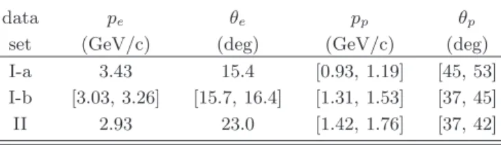
TABLE III: Summary of the kinematical settings for each data set. The nominal beam energy is Ebeam = 4.045 GeV

(see section IV D for actual values). peand θeare the central

momentum of the HRS-E spectrometer and its angle w.r.t. the beamline (electron side). ppand θpare the same variables

on the proton side, i.e. for the HRS-H spectrometer.

data pe θe pp θp

set (GeV/c) (deg) (GeV/c) (deg)

I-a 3.43 15.4 [0.93, 1.19] [45, 53]

I-b [3.03, 3.26] [15.7, 16.4] [1.31, 1.53] [37, 45]

II 2.93 23.0 [1.42, 1.76] [37, 42]

Data acquisition was performed with the CODA soft-ware developed by CEBAF [48]. The trigger setup in-cludes several types, among which T1 and T3 are single-arm HRS-E and HRS-H good triggers. The T5 triggers, formed by the coincidence between T1 and T3, are the main ones used in the physics analysis. For each event the raw information from the detectors and the beam posi-tion devices is written on file. Scalers containing trigger rates and integrated beam charge are inserted periodi-cally in the datastream, as well as various parameters from the EPICS slow control system. Special runs were recorded to study spectrometer optics.

IV. DATA ANALYSIS

This section describes the main steps that were nec-essary to reach the accurate measurement of the (ep → epγ) differential cross section: raw-level processing, event reconstruction, analysis cuts, and acceptance calculation.

A. Beam charge, target density and luminosity The electron beam current is measured by two reso-nant cavities (Beam Charge Monitors BCM) placed up-stream of the Hall A target. The signal of each cavity is sent to different electronic chains. In the experiment, the main measurement of the beam charge used the up-stream cavity and the chain consisting in an RMS-to-DC converter followed by a Voltage-to-Frequency converter (VtoF), generating pulses that are counted by a scaler. The content of the VtoF scaler was written on the runfile every 10 seconds. At the end of each run one obtained in this way the integrated charge of the run. The BCM were calibrated twice a day against the Unser monitor, located between the two cavities and measuring the beam current in absolute. The procedure also implied the of-fline calibration of the VtoF converter. Beam currents ranged from 30 to 100 µA with an average of 70 µA, and the integrated charge per run was determined with an accuracy of 0.5%.

The experiment used the 15 cm long liquid hydrogen cell (“beer can”). It was kept at a constant temperature T = 19.0 K and pressure P = 1.725 bar, yielding a den-sity ρ0= 0.0723 g.cm−3 at zero beam current [49]. The

beam was rastered on the target in both transverse di-rections in order to avoid local boiling of the hydrogen. Studies based on the data of this experiment [45] showed that density losses reached at maximum 1% for a beam current of 100 µA, so the target boiling effect was con-sidered to be negligible and the density was taken equal to ρ0 in the analyses.

The luminosity L needed for cross section measure-ments is obtained on a run-per-run basis. Based on the above considerations, it is determined with an accuracy of ∼ ± 1%. Typical values of instantaneous luminosities are of the order of 2 to 4×1038 _cm−2_·s−1_.

B. Rate corrections

The raw event rate is obtained by counting the number of T5 events, i.e. the coincidence triggers between the two spectrometers. Several correction factors have to be applied to this rate.

The first correction is due to trigger inefficiency, com-ing from the scintillators of the detector package. It is obtained by studying the single-arm “junk triggers” T2 (electron side) and T4 (hadron side), which record all configurations other than normal in the scintillators. The normal configuration (T3 or T5) is a coincidence between paddles in the S1 and S2 planes in an allowed geometri-cal configuration (“S-ray”), each paddle signal requiring the coincidence between its left and right phototubes. Among the junk triggers, there are some good events, typically with a hit missing in the scintillator paddles. We identify them by a “clean-up” procedure, consisting in the additional requirement of a valid track in the VDCs and a Cerenkov signal in the electron arm. The scintil-lator inefficiency is then defined as the number of such good T2 or T4 events, relative to the number of (T1+T5) or (T3+T5) events in the same clean-up conditions. The inefficiency is calculated independently for both planes S1 and S2 in each arm. It is binned in the x (dispersive) and y (transverse) coordinates in each plane, to account for local variations. The observed inefficiency was usu-ally of the order of one percent, reaching occasionusu-ally 10% locally in the electron arm [50]. This commissioning problem was fixed after our experiment.

The second correction concerns the acquisition dead-time. For each run, a scaler counts the number S5of T5

events at the output of the trigger logic. Among these events, only N5 (< S5) are written on file due to the

deadtime of the [acquisition+computer] system. The cor-rection consists in multiplying the event rate by the ratio S5/N5. The deadtime depends on the beam current; it

varied between 5% and 40% in the experiment.

The third correction comes from the deadtime of the trigger electronics itself (EDT). It was not measured di-rectly during the experiment but determined afterwards. The EDT estimation is based on a fit to the actual rates in the scintillator paddles, using the strobe rate of each spectrometer. This fit was established in later experi-ments when the strobe rate was inserted in the datas-tream [51]. The resulting correction is of the order of 1-3% in our case.

The tracking inefficiency is considered to be negligible, in the sense that for a real particle, the tracking algorithm basically always finds at least one track in the focal plane, which allows to process the event further. This is due to the good efficiency per wire in the VDCs.

Finally, another small correction of the order of 1% is applied to account for the losses of protons by nuclear interactions in the target and spectrometer windows.

The uncertainty on the event rate, after having cor-rected for all the above inefficiencies, is estimated to be smaller than 0.5% in relative.

C. Event reconstruction

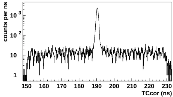
The Hall A analyzer ESPACE processes the raw detec-tor signals and builds all the first-level variables of the event: coincidence time, beam position on target, three-momentum vector of the detected particles at the vertex point, etc. Figure 5 shows a typical coincidence time spectrum between the HRS-E and HRS-H. The central peak allows to select the true coincidences. Random coin-cidences under the peak are subtracted using side bands. In the plateau one clearly sees the 2 ns microstructure of the beam, corresponding to Hall A receiving one third of the pulses of the 1497 GHz CW beam.

1 10 102 103 150 160 170 180 190 200 210 220 230 TCcor (ns) counts per ns

FIG. 5: Coincidence time spectrum of data set I-a. The cen-tral peak is 0.5 ns wide in rms.

In the analyses presented here, particle identification in the detectors is basically not needed. This is because the kinematical settings of VCS near threshold (cf. Ta-ble III) are close to ep elastic scattering, therefore the true coincidences between the two spectrometers are es-sentially (e, p) ones. The other true coincidences that could be considered are of the type (e−_{, π}+_{) or (π}−_{, p),}

coming from single or multiple pion production processes. However, such events either do not match the accep-tance settings (case of single charged-pion electropro-duction) or they yield missing masses which are beyond one pion mass, i.e. far from the VCS region of interest (case of multiple pion production). Therefore detectors such as the gas Cerenkov counter or the electromagnetic calorimeter in the HRS-E were essentially not used, and only the information from the VDCs and the scintillators in both arms were treated. As a verification, however, the analysis of data set II was performed with and without requiring a signal in the Cerenkov counter in the HRS-E, and the results were found unchanged.

Due to the extended size of the target and the rather large raster size (∼ ± 3-5 mm in both directions), it is important to know the interaction point inside the hy-drogen volume for each event. This point is character-ized by its coordinates (xv, yv, zv) in the Hall A

labora-tory frame. The coordinates transverse to the beam axis, horizontal xv and vertical yv, are obtained from the two

for a large fraction of the data taking, the BPM infor-mation was accidentally desynchronized from the event recorded by CODA. A special re-synchronization proce-dure [46, 52] was established offline by coupling the BPM to the raster information (which is always synchronized with the event). Then the BPMs could be used, yielding xv and yvin absolute to better than ± 0.5 mm event per

event.

The calculation of the longitudinal coordinate zv

re-quires information from the spectrometers. It is obtained by intersecting the beam direction with the track of one of the two detected particles. For this task the HRS-E was chosen, since it has the best resolution in horizontal coordinate, i.e. the variable noted ytgin the spectrometer

frame. The resolution in ytg is excellent, about 0.6 mm

in rms for the HRS-E (and twice larger for the HRS-H). The particle reconstruction proceeds as follows. In each arm the particle’s trajectory is given by the VDCs in the focal plane. This “golden track” is characterized by four independent variables (x, y, θ, ϕ)f p. These variables

are combined with the optic tensor of the spectrometer to yield four independent variables at the target: the rel-ative momentum δp/p, the horizontal coordinate ytg, and

the projected horizontal and vertical angles, θtg and ϕtg,

in the spectrometer frame. A fifth variable xtg

character-izing the vertical extension of the track is calculated using the beam vertical position, and allows to compute small extended-target corrections to the dispersive variables θtg

and δp/p. The total energy of the particle is then deter-mined from its momentum and its assumed nature (e in HRS-E or p in HRS-H). It is further corrected for energy losses in all materials, from the interaction point to the spectrometer entrance. At this level the four-momentum vectors of the incoming electron, scattered electron and outgoing proton: k, k′ _{and p}′_{, respectively, are known at}

the vertex point. One can then compute the full kinemat-ics of the reaction ep → epX and a number of second-level variables.

For the physics analyses, the main reconstructed vari-ables are Q2_{, W, ǫ, q}

c.m. on the lepton side, and the

four-momentum vector of the missing system X: pX =

k + p − k′ _{− p}′_{. This four-vector is transformed from}

the laboratory frame to the CM, where one calculates the angles of the missing momentum vector ~pXc.m.w.r.t.

the virtual photon momentum vector ~qc.m.. These angles,

polar θc.m. and azimuthal ϕ (see Fig. 2), and the

modu-lus of the missing momentum, which represents q′ c.m. in

the case of VCS, are the three variables used to bin the cross section.

Other second-level variables are important for the event selection as well as for the experimental calibra-tion. The first one is the missing mass squared M2

X =

(k + p − k′_{− p}′₎2_{. In the experimental M}2

X spectrum,

a photon peak and a π0 _{peak are observed,}

correspond-ing to the physical processes ep → epγ and ep → epπ0

(see Fig. 7). A cut in M2

X is thus necessary to select the

reaction channel.

Two other variables, of geometrical nature, have

proven to be useful. The first one, xdif, compares two

independent determinations of the horizontal coordinate of the vertex point in the Hall A laboratory frame: the one measured by the BPMs (xv) and the one obtained by

intersecting the two tracks measured by the spectrome-ters, and called x2arms. The distribution of the difference

xdif = x2arms− xv is expected to be a narrow peak

cen-tered on zero. The second geometrical variable, Ydif, will

be described in section IV E.

D. Experimental calibration

A lot of experimental parameters have to be well cali-brated. At the time of the experiment, the existing optic tensors of the spectrometers were not fully adapted to an extended target; it was necessary to optimize them. Using dedicated runs, new optic tensors were determined for the VCS analysis [53]. They were obtained in both arms for our designed momentum range, and they clearly improved the resolution of the event reconstruction.

A number of offsets, of either geometrical or kinemati-cal origin, also had to be adjusted. Among the geometri-cal offsets, some were given by the CEBAF surveys, such as the target and collimator positions. Others, such as the mispointing of the spectrometers, were recorded in the datastream, but their reading was not always reli-able and some of them had to be adjusted by software. One should note that not all offsets have to be known in absolute; what is needed is the relative coherence be-tween target position, beam position and spectrometer mispointing. The consistency checks were made on the distribution of the zv and xdif variables (defined in

sec-tion IV C) for real events. The main geometrical offset was found to be a horizontal mispointing of the HRS-E by 4 mm.

The kinematical offsets consist in small systematic shifts in the reconstructed momentum and angles of the particles at the vertex point. They are mainly due to i) a beam energy uncertainty (the beam energy mea-surements described in [42] were not yet operational), ii) residual biases in the optic tensors, iii) field repro-ducibility in the spectrometer magnets. The adjustment of these offsets is based on the optimization of the peaks in missing mass squared, in width and position, for the two reactions ep → epγ and ep → epπ0 _{simultaneously.}

This procedure yields a coherent set of offsets for each setting [54]. An overview of the results is presented in Table IV. All kinematical offsets were found to be small, except for the beam energy which was significantly below the nominal value from the accelerator, by about 10-16 MeV (see Fig. 6).

E. Analysis cuts

The offsets described above were established using clean event samples. However, the raw coincidences are

-15 -10 -5 0 0 5 10 15 20 25 30 35 40 45 Setting Number ∆ Ebeam

(MeV) I-a I-b

part 1 II I-b part 2 -15 -10 -5 0 0 5 10 15 20 25 30 35 40 45

FIG. 6: The fitted offset in beam energy, ∆Ebeam, versus the

setting number (time-ordered). There is one point per setting. The various data sets are delimited by the vertical lines. The horizontal line at ∆Ebeam = 0 corresponds to the nominal

beam energy from the accelerator, Ebeam= 4.045 GeV.

TABLE IV: Global results for the fitted offsets on the seven variables: beam energy, particle momenta (pe, pp) and

parti-cle angles. ϕtg(e), ϕtg(p)(resp. θtg(e), θtg(p)) are the horizontal

(resp. vertical) angles of the particle’s track in the spectrom-eter frame. Some offsets have to be fixed in order to ensure the fit stability [54]. The range in brackets indicates setting-to-setting variations of the offsets.

variable range found estimated uncertainty

for the offset on the offset

Ebeam [-16, -10] MeV ± 2 MeV

pe 0 (fixed) ± 0.3 MeV/c pp [-1.5, +1.5] MeV/c ± 0.5 MeV/c ϕtg(e) [0, +0.1] mr ± 0.3 mr ϕtg(p) [-1.7, -0.7] mr ± 0.3 mr θtg(e) [-1.6, -0.5] mr ± 0.5 mr θtg(p) 0 (fixed) ± 0.5 mr

not so clean, as can be seen e.g. from the spectrum in the insert of Fig. 7 (top plot). The photon peak is con-taminated by a large broad bump centered near -15000 MeV2_{. These events are mostly due to ep elastic}

scatter-ing with the final proton “punchscatter-ing through” the HRS-H entrance collimator. They require specific cuts in order to be eliminated. A key condition for the VCS analysis is to obtain a well-isolated photon peak in the M2

X

spec-trum ( Fig.7, histogram 5). The cuts necessary to reach this goal are described below.

First, standard acceptance cuts are applied in each arm. They use essentially the Hall A R-functions [55], which are a way to handle complex cuts in a multi-dimensional space. In the R-function approach, the prob-lem is transformed into the calculation, for each detected particle, of its ”distances” to the acceptance boundaries, and the combination of these distances into one single function. This R-function takes continuous values: posi-tive inside the acceptance domain, negaposi-tive outside, and equal to zero on the boundaries; it can then be used as a one-dimensional cut (e.g., here we require R-function

0 500 1000

counts per 300 MeV

2 0 500 1000 ₁ 2

γ

π

o

M

_(GeV

₎

(c)

(a)

(b)

FIG. 7: (Color online) A sample of data set II: the experimen-tal spectrum of the missing mass squared at various levels of cuts, added successively and labelled from 1 to 5. (a): the raw coincidences (1) and adding the R-function cut (2). (b): adding the conditions W > 0.96 GeV (3), Ydif < −0.012 m

(4) and |xdif| < 3 mm (5) (see the text for the description of

the variables). The insert (c) shows histogram 1 in full scale abscissa.

>0). We also use additional -and largely redundant-contour cuts in two dimensions among the (δ, y, θ, ϕ)tg

quadruplet, and restricted apertures in the plane of the entrance collimators. We note that the target endcaps, located at ± 75 mm on the beam axis, are not seen in coincidence, due to the rather large HRS-H spectrometer angles; so a cut in zv is not necessary. The effect of the

standard acceptance cuts is shown in Fig. 7 (histogram 2). Clearly they are not sufficient to fully clean the M2

X

spectrum, and supplementary cuts are necessary. Normally, the protons coming from ep elastic scatter-ing are too energetic to be in the momentum acceptance of the HRS-H for our chosen settings. However, some of these protons go through the material of the entrance col-limator (tungsten of 80 mm thickness) where they scatter and lose energy, after which they enter the acceptance and are detected. This problem cannot be avoided, since VCS near threshold is by nature close to ep elastic scat-tering.

As a result, a prominent ep elastic peak is seen in the W -spectrum for true coincidences, at the raw level and even after having applied the standard acceptance cuts, cf. Fig. 8. A striking evidence for “punch-through” pro-tons is also provided by the inserts in Fig. 8. These plots show the 2D impact point of the proton in the HRS-H collimator plane, calculated in a particular way. Here we do not use the information from the HRS-H, we only use the HRS-E informations and the two-body ep elastic kinematics. Knowing the vertex point (from the HRS-E and the beam), the beam energy and the scattered elec-tron angles, one can deduce the point where the proton from ep elastic kinematics should have hit the collima-tor. This hit point is characterized by its coordinates xc

(vertical) and yc (horizontal) in the HRS-H

spectrome-ter frame. For events in the elastic peak of Fig. 8, the (xc, yc) distribution (insert (r)) reproduces faithfully the

structure of the collimator material, proving that these are indeed protons punching through the collimator. The R-function cut is able to remove part of these events, but keeps the punching through the upper and lower parts of the collimator, as shown by insert (a). Of course our purpose here is only illustrative; these events are not a concern, since they are removed by a simple cut in W around the elastic peak. The result of such a cut in terms of missing mass squared is displayed as histogram 3 of Fig. 7.

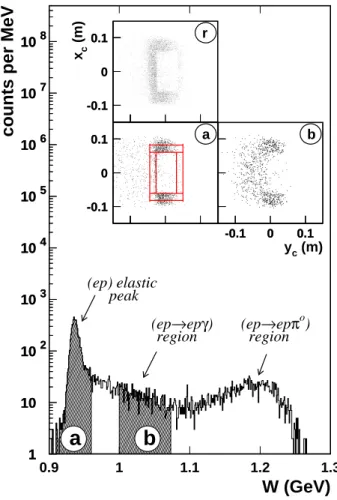
The main concern is that there are also “punch-through” protons at higher W , as evidenced by insert (b) of Fig. 8, where an image of the collimator material is still present. This region in W is the far radiative tail of the ep elastic process; in other words it is the kinematical region of interest for VCS, therefore one cannot use a cut in W . Nevertheless these “punch-through” events must be eliminated, because i) they are badly reconstructed and ii) the simulation cannot reproduce them (our sim-ulation, which is used to obtain the cross section, see sections IV F and IV G, considers only perfectly absorb-ing collimators). To this aim, a more elaborate cut has been designed which we now describe.

For a “punch-through” proton, the variables (δ, y, θ, ϕ)tg obtained directly from the HRS-H are

usually severely biased, due to the crossing of a thick collimator. Therefore they are of little use, except for one particular combination: yHadron

collim = ytg + D · ϕtg,

where D is the distance from the target center to the collimator. This quantity yHadron

collim gives the horizontal

impact coordinate of the proton track in the collimator plane, as measured directly by the HRS-H. It is an unbi-ased variable, even for a “punch-through” proton. This is because the collimator plane is where the distortion happened. The reconstruction of the proton trajectory, which is performed backwards, from focal plane to target, is correct down to the entrance collimator (and biased further down to the target). The idea is then to compare this quantity yHadron

collim with the “elastic”

coor-dinate yc calculated just above. For “punch-through”

protons the two calculations turn out to be in close

1 10 102 103 104 105 106 107 108 0.9 1 1.1 1.2 1.3

W (GeV)

counts per MeV

1 10 102 103 104 105 106 107 108

a

b

FIG. 8: (Color online) A sample of data set II: the experimen-tal W spectrum for the coincidence events after the R-function cut. The inserts show the proton impact in the HRS-H colli-mator calculated “elastically” (see text). Events in inserts (a) and (b) correspond to the two hatched zones of the histogram: the ep elastic peak (W < 0.96 GeV (a)) and a typical VCS region (1.0 < W < 1.073 (b)). In insert (a) a sketch of the tungsten collimator is drawn. The upper insert (r) shows the ep elastic events before applying the R-function cut.

agreement, hence the difference Ydif = yc − ycollimHadron

peaks at zero. We point out that this comparison can only be done for the horizontal coordinate, not in vertical, due to the fact that the vertical extension xtg

is intrinsically not measured by the spectrometers. Fig. 9 shows the Ydif distribution. Clean VCS events

cover smoothly the Ydif < 0 region (dashed histogram),

while experimental events (solid histogram) exhibit an extra-peak centered on zero. This peak corresponds to “punch-through” protons and is most efficiently elimi-nated by requiring the condition Ydif < −12 mm. The

rejected events (insert (b)) again clearly reveal the image of the tungsten collimator. The retained events (insert (a)) show a smooth distribution in the (xc, yc) plane, well

reproduced by the VCS simulation. The Ydif cut is

defi-nitely efficient in isolating a clean photon peak, as shown by histogram 4 of Fig. 7.

0 50 100 150 200 250 300 350 400 450 -0.2 -0.1 0 0.1 Ydif (m) counts per 0.35 mm 0 50 100 150 200 250 300 350 400 450 -0.2 -0.1 0 0.1 -0.1 0 0.1 -0.1 0 0.1 y_c (m) xc (m) -0.1 0 0.1 -0.1 0 0.1

a

b

FIG. 9: (Color online) A sample of data set II: the experi-mental Ydif spectrum (see text) for coincidence events

sur-viving the AND of the three following cuts: R-function > 0, −5000 < M2

X < 5000 MeV2 and W > 0.96 GeV (solid

his-togram). The inserts show the “elastically calculated” proton impact in the HRS-H collimator (see text) for Ydif< −0.012m

(clean events, plot (a)) and for Ydif > −0.012 m

(punch-through protons, plot (b)). The dashed histogram corre-sponds to the VCS simulation with the same three cuts.

Lastly, to obtain histogram 5 in Fig. 7 the geometrical variable xdif (cf. section IV C and Fig. 10) is selected

around the central peak, i.e. in the interval [-3,+3] mm, completing the removal of badly reconstructed events. It is worth noting that these two last cuts in Ydif and xdif

(which are correlated but not equivalent), owe their effi-ciency to the excellent spectrometer intrinsic resolution in ytg, already emphasized in section IV C.

After the above cuts, a small fraction of events (≤ 5%) still have more than one track in one arm or the other. The number of tracks is given by the VDC algorithm to-gether with the parameters of the “golden track”. One may either keep these multi-track events, or reject them and renormalize the rate accordingly, based on the fact that these are still good events, just less clean. This sec-ond method was chosen, except for data set II where the multi-track events are in very small proportion (≤ 0.5%). Finally, events are selected in a window in M2

X around

the photon peak, typically [-5000,+5000] MeV2_{, and in}

certain W -range. The lower bound in W corresponds to q′

c.m. = 30 MeV/c and the upper bound is imposed

de-pending on the type of analysis, LEX or DR (cf. Fig.3). The (very few) random coincidences that remain are sub-tracted. After all cuts, the final event statistics for the analyses are about 35000 (data set I-a), 13000 (data set

I-b) and 25000 (data set II).

F. Monte-Carlo simulation

The experimental acceptance is calculated by a ded-icated Monte-Carlo simulation which includes the ac-tual beam configuration, target geometry, spectrome-tor acceptance and resolution effects. It is described in detail in [56] and we just recall here the main fea-tures. The ep → epγ kinematics are generated by sam-pling in the five variables of the differential cross section d5_σ/dk′

elabdΩ′elabdΩγc.m.. The scattered electron

momen-tum and angles in the laboratory frame define the virtual photon, then with the angles of the Compton process in the CM one can build the complete 3-body kinematics. Events are generated according to a realistic cross sec-tion, the (BH+Born) one, over a very large phase space. The emitted electron and proton are followed in the tar-get materials, and the event is kept if both particles go through the [collimator+spectrometer] acceptance. One forms the four target variables (δ, y, θ, ϕ)tg of each track

and implements measurement errors on these variables in order to reproduce the resolution observed experimen-tally. Finally, one proceeds to the event reconstruction and analysis cuts in a way similar to the experiment.

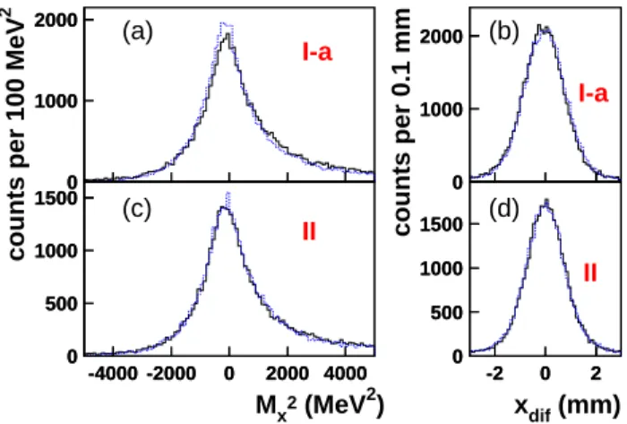
As an example, Fig. 10 shows the distribution of the variables M2

X and xdif, for two VCS data sets after all

cuts. These variables are not sensitive to the details of the physics; with an infinitely good resolution they should be delta-functions, therefore they characterize the resolution achieved in the experiment. The agreement between the experimental and simulated data is very good not only in the main peak but also in the tails of the distributions, which is of importance as far as cuts are concerned. The excellent resolution achieved in missing mass squared allows to cleanly separate the (ep → epγ) and (ep → epπ0) channels. The residual contamination of π0_{events under the γ peak is negligible for the settings}

analyzed here: simulation studies show that it is smaller than 0.5 %.

The radiative corrections are performed along the lines of ref. [57], based on the exponentiation method. The simulation takes into account the internal and external bremsstrahlung of the electrons, because the associated correction depends on the acceptance and the analysis cuts. This allows the simulation to produce a realistic radiative tail in the M2

X spectrum, visible on the right

side of the peak in Fig. 10-left. The remaining part of the radiative effects, due to virtual corrections plus real corrections which do not depend on experimental cuts, is calculated analytically. It is found to be almost constant for the kinematics of the experiment [58]: Frad ≃ 0.93,

therefore it is applied as a single numerical factor, such that dσcorrected= dσraw×Frad in each physics bin. The

estimated uncertainty on Frad is of the order of ±0.02,

i.e. it induces a ±2% uncertainty on the cross section, globally on each point and with the same sign.

0 1000 2000 I-a 0 1000 2000

counts per 100 MeV

2 0 1000 2000 I-a 0 1000 2000 counts per 0.1 mm 0 500 1000 1500 -4000 -2000 0 2000 4000 II 0 500 1000 1500 -4000 -2000 0 2000 4000 M_x2 _(MeV2₎ 0 500 1000 1500 -2 0 2 II 0 500 1000 1500 -2 0 2 x_dif (mm) (a) (b) (c) (d)

FIG. 10: (Color online) Data sets I-a (top) and II (bottom) after all cuts: comparison of experiment (solid histogram) and simulation (dotted histogram). (a),(c): the missing mass squared in the VCS region; the peak FWHM is about 1650 MeV2. (b),(d): the geometrical variable xdif (see text); the

peak FWHM is about 1.9 mm.

G. Cross section determination

We first explain the principle of the cross section deter-mination in a bin, and then the chosen binning in phase space. In a given bin, after all cuts and corrections to the event rate, the analysis yields a number of experi-mental VCS events Nexp corresponding to a luminosity

Lexp. Similarly, the simulation described in section IV F

yields a number of events Nsim corresponding to a

lu-minosity Lsim. The experimental cross section is then

obtained by: d5σEXP ₌ Nexp Lexp · Lsim Nsim · d5σsim(P0) , (7)

where the factor [Lsim·d5σsim(P0)/Nsim]−1 can be seen

as an effective solid angle, or acceptance, computed by the Monte-Carlo method. d5_σ

sim(P0) is the cross

sec-tion used in the simulasec-tion, at a fixed point P0 that can

be chosen freely. As explained in [56], this method is justified when the shape of the cross section d5_σ

sim is

realistic enough, and it gives rise to a measured cross sec-tion (d5_σ/dk′

elabdΩ′elabdΩγc.m.) at some well-defined fixed

points in phase space.

These points are defined by five independent variables. The most convenient choice w.r.t. the LET formulation is the set (qc.m., q′c.m., ǫ, θc.m., ϕ). We will work at fixed

qc.m. and fixed ǫ, and make bins in the other three

vari-ables. For the subsequent analyses, instead of the stan-dard (θc.m., ϕ) angles, another convention (θ′c.m., ϕ′c.m.) is

chosen. It is deduced from the standard one by a simple rotation: the polar axis for θ′

c.m. is chosen

perpendicu-lar to the lepton plane, instead of being aligned with the ~

qc.m.vector (see Appendix A for more details). This new

system of axis allows an angular binning in which the

direction of ~qc.m. does not play a privileged role. Due

to the narrow proton cone in the laboratory, the angular acceptance in the CM is almost complete for data sets I-a and II. This is illustrated in Fig. 11. We note that the two peaks of the BH cross section, located in-plane, are out of the acceptance (see also Fig. 12). This is on purpose, since in these peaks the polarizability effect in the cross section vanishes. When W increases, the ac-ceptance reduces to more backward scattering angles [6]. Table X in Appendix A summarizes the bin sizes and the chosen fixed points in phase space. As a consequence, the results of the experiment are obtained at two fixed values of Q2_{: 0.92 and 1.76 GeV}2_.

0 50 100 150 -100 0 100 (deg) Θ , (deg) c.m. c.m. 0 50 100 150 -100 0 100

FIG. 11: Accepted phase space in (θ′

c.m., ϕ′c.m.) for data set

I-a. The two crosses denote the position of the BH peaks and the horizontal line corresponds to in-plane kinematics (θ′

c.m.= 90◦or ϕ = 0◦and 180◦).

In eq.(7) the cross section d5_σEXP _{is first calculated}

using the BH+Born cross section for d5_σ

sim, i.e. no

po-larizability effect is included in the simulation. Then, to improve the accuracy, we include a Non-Born term in d5_σ

sim, based on what we find for the polarizabilities

at the previous iteration. Below the pion threshold this Non-Born term is the first-order LEX term of eq.(1). For the region above the pion threshold, this Non-Born term is computed using the dispersion relation formalism, and the iterations are made on the free parameters of the model. In all cases this iterative procedure shows good convergence.

H. Sources of systematic errors

The systematic errors on the cross section come from three main sources: 1) overall absolute normalization, 2) beam energy, 3) horizontal angles of the detected parti-cles.

The uncertainty in the absolute normalization has principally three origins: the radiative corrections known to ±2%, the experimental luminosity known to ±1%, and the detector efficiency corrections known to ±0.5% (see previous sections). Added in quadrature, they give a overall normalization error of ±2.3%, applying to all cross-section points with the same sign.

The uncertainty in the beam energy, deduced from the offsets study of section IV D, is taken equal to ±2 MeV. The uncertainty in horizontal angles essentially reflects the accuracy of the optic tensors and is taken equal to ±0.5 mr in each arm. To study the systematic error in-duced by the beam energy or the horizontal angles, the experimental events are re-analyzed with these param-eters changed, one by one separately, by one standard deviation. One obtains in each case a set of modified cross-section data; in certain cases we observe a change of shape of the cross section. One can summarize these ef-fects by saying that error sources 2) and 3) taken together are equivalent to an average systematic uncertainty of ± 6% (resp. ± 7%) on the cross section, for data set I-a (resp. II). These errors include substantial point-to-point correlations.

Systematic errors on the physics observables will be discussed in sections V B 1 and V B 2.

I. Choice of proton form factors

The proton elastic form factors Gp_E and Gp_M are an important input in an analysis of VCS at low energy. Indeed they are needed to calculate the BH+Born cross section, which is at the basis of the low-energy expansion. Throughout these analyses the form factor parametriza-tion of Brash et al. [59] was chosen. It provided the first fit consistent with the observed departure from one of the ratio µpGpE/G

p

M in our-Q2 range [60, 61].

The VCS structure functions and GPs are always ex-tracted by measuring a deviation from the BH+Born pro-cess –either analytically as in the LEX approach, or in a more complex way as in the DR approach. This state-ment means that the GP extraction is sensitive to both cross sections, d5σEXP _{and d}5_σBH+Born_{: a 1% change}

on d5_σEXP _{has the same impact as a 1% change on}

d5_σBH+Born_{. This last cross section is not known with}

an infinite accuracy, due to uncertainties on the proton form factors. Therefore a systematic error should be at-tached to our calculation of d5_σBH+Born_{. To treat it in}

a simplified way, we consider that form factor uncertain-ties are equivalent to a global scale uncertainty of ± 2% on d5_σBH+Born_{. Then, when dealing with the}

extrac-tion of the physics observables (secextrac-tions V B and V C), this effect can be put instead on d5_σEXP_{, i.e. it can be}

absorbed in the overall normalization uncertainty of the experiment. Consequently, in sections V B and V C, we will simply enlarge the systematic error due to normal-ization (source # 1 in section IV H) from ± 2.3% to ± 3% (= quadratic sum of 2.3% and 2%).

V. RESULTS AND DISCUSSION

We first present the results for the photon electropro-duction cross section. Then the VCS structure functions and the GPs are presented and discussed. The main

re-sults for these observables are contained in Tables V, VII and IX.

A. Theep → epγ cross section

The experiment described here provides a unique set of data for VCS studies, combining altogether a large an-gular phase space (including out-of-plane angles), a large domain in CM energy (from the threshold to the Delta resonance) and an access to the high-Q2 _{region. Our}

cross-section data are reported in Tables XIII to XVII of Appendix C.

1. Angular and energy dependence

Selected samples of our results are presented in Figs. 12 to 15. Figure 12 shows the measured cross section for the highest value of q′

c.m. below the pion threshold (105

MeV/c). The in-plane cross section (θ′

c.m. = 90◦) rises

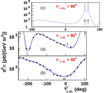
by seven orders of magnitude in the vicinity of the BH peaks, which are indicated by the two arrows. The out-of-plane cross section has a much smoother variation. As expected, the measured values exhibit a slight departure from the BH+Born calculation, due to the polarizabili-ties. The magnitude of this effect is best seen in Fig. 13 which depicts the deviation of the measured cross section relative to BH+Born: in-plane this ratio varies between -5% and +20%, except in the dip near ϕ′

c.m. = −200◦

(or +160◦_{) where it reaches larger values. This complex}

pattern is due to the VCS-BH interference. Out-of-plane the polarizability effect is much more uniform, with an average value of ∼ −10%.

Another selected sample of results is displayed in Fig. 14, this time above the pion threshold (at q′

c.m.= 215

MeV/c) and for backward angles of the outgoing photon. There, the first-order term of the LET becomes clearly insufficient to explain the observed cross section, while the calculation of the DR model, which includes all or-ders, performs quite well. The energy dependence of the cross section, i.e. the dependence in q′

c.m. or W , is

gov-erned by a strong rise when q′

c.m.tends to zero due to the

vicinity of the ep elastic scattering, and a resonant struc-ture in the region of the Delta(1232). These feastruc-tures can be seen in Fig. 18.

2. Overall normalization test

The effect of the GPs in the photon electroproduction cross section roughly scales with the outgoing photon en-ergy q′

c.m.. Therefore the physics results are determined

essentially from the bins at high q′

c.m., which have the

highest sensitivity to the GPs. At our lowest q′ c.m. of

45 MeV/c, this sensitivity is much reduced, and one can test another aspect of the experiment, namely the overall normalization.

1 102 104 106 108 -180 0 180 1 102 104 106 108 θ , c.m. = 90 o 10 102

d

σ

(pb/(GeV sr

))

(deg)

FIG. 12: (Color online) Data set I-a below the pion threshold, at q′

c.m.= 105 MeV/c. The (ep → epγ) cross section is shown

in-plane (θ′

c.m. = 90◦, (a)) and out-of-plane (θ′c.m. = 40◦,

(b)). The dotted curve is the BH+Born calculation. The solid curve includes the first-order GP effect calculated using our measured structure functions. The errors on the points are statistical only, as well as in the six next figures. The upper plot (c) shows the in-plane BH+Born cross section with a full-scale ordinate and the more traditional abscissa running between ϕ′ c.m.= −180◦ and ϕ′c.m.= +180◦. 0 0.5 1 1.5 2 0 0.5 1 1.5 2 θ , c.m. = 90 o -0.2 0 0.2 0.4 -200 -100 0 100

(deg)

ratio

FIG. 13: (Color online) The ratio (dσEXP ₋

dσBH+Born)/dσBH+Born for the data points of the pre-vious figure. The solid curve shows the first-order GP effect calculated using our measured structure functions.

When q′

c.m. tends to zero, d5σEXP formally tends to

the known BH+Born cross section. This is a model-independent statement, best illustrated by the LEX ex-pansion of eq.(1). At q′

c.m. = 45 MeV/c, the first-order

term (q′

c.m.· φ · Ψ0), calculated using our measured values

for the structure functions, is very small. It is about 2%

10 102 -200 -150 _c.m. (deg) d 5 σ (pb/(GeV sr 2 ))

I-a

II

FIG. 14: (Color online) The (ep → epγ) cross section for data sets I-a (plot (a)) and II (plot (b)) at q′

c.m. = 215 MeV/c,

in-plane (θ′

c.m. = 90◦) as a function of ϕ′c.m.. The dashed

curve is the DR model calculation, with parameter values as fitted in the experiment. The dotted (resp. solid) curve is the BH+Born cross section (resp. plus a first-order GP effect).

10 102 d 5 σ (pb/(GeV sr 2 )) θ ,c.m. = 90 o 10 102 102 103 -200 -100 0 100 _c.m. (deg) θ , c.m. = 40 o 102 103 1.6 1.8 2 2.2 2.4 0.96 1 1.04 F_norm

χ

FIG. 15: (Color online) Data set I-a. The (ep → epγ) cross section at the lowest q′

c.m.of 45 MeV/c, for in-plane (a) and

out-of-plane (b) kinematics. The solid curve is the (BH+Born + first-order GP) cross section. The right plot (c) shows the reduced χ2of the normalization test.

of the BH+Born cross section, and it remains essentially unchanged when the structure functions are varied by one standard deviation. Therefore, at the lowest q′

c.m. the

comparison of the measured cross section dσEXP _with

the cross section d5σcalc _{calculated from eq.(1):}

d5σcalc= d5σBH+Born + q′c.m.· φ · Ψ0,

is essentially a test of the absolute normalization of the experiment. In practice, one allows dσEXP _{to be}

renor-malized by a free factor Fnorm, and a χ2is minimized

be-tween dσEXP _{and dσ}calc_{as a function of F}

norm. The test

is performed on data sets I-a and II at the lowest q′ c.m.;

the χ2min is always found for Fnorm in the range [0.99,

1.01]. An example is given in Fig. 15. To conclude, our cross-section data need very little renormalization, less than 1%. This means in particular that there is a good