Applicability of linear analysis in probabilistic estimation of seismic building damage to reinforced-concrete structures

(1)

Applicability of Linear Analysis in Probabilistic Estimation of

Seismic Building Damage to Reinforced-Concrete Structures

By

Timothy P. James B.S. Civil Engineering

University of Alaska, Anchorage, 2004

SUBMITTED TO THE DEPARTMENT OF CIVIL AND ENVIRONMENTAL ENGINEERING IN PARTIAL FULFILLMENT OF THE REQUIREMENTS FOR THE

DEGREE OF

MASTER OF ENGINEERING IN CIVIL AND ENVIRONMENTAL ENGINEERING

AT THE

MASSACHUSETTS INSTITUTE OF TECHNOLOGY S s: UTITUTE

JUNE 2012

Applicability of Linear Analysis in Probabilistic Estimation of

Seismic Building Damage to Reinforced-Concrete Structures

By

Timothy P. James

Submitted to the Department of Civil and Environmental Engineering on May 11, 2012 in Partial Fulfillment of the Requirements for the Degree of Master of Engineering in Civil and

Environmental Engineering

Abstract

As design has moved from strength based to performance based, there has been an effort to relate building response to damage. Because decision-makers typically consider human lives, property damage and cost, setting performance requirements in terms of the damage that a building is likely to sustain over time and its associated cost is more relevant to them. The Pacific Earthquake Engineering Research Center (PEER) has developed a computationally expensive methodology for estimating cumulative damage to a structure over its lifetime. This thesis shows that linear analysis produces results within an acceptable margin of error when substituted for excessively accurate non-linear, resulting in significant time savings.

Thesis Supervisor: Jerome J. Connor

(4)

(5)

To Yuko:

1l0 & ) 9

~~W-~~~

{±1~

2O -CLI 9

MIT

zb/Z D

4E

MI

To Yoko and Sunshine: I am words can show. Thank you your thoughts and feelings.

so proud of both of you and love you more than for always showing confidence in me and sharing I love you.

To Pierre Ghisbain: Thank you for giving me direction and focus for this thesis. I could not have completed this without your guidance and thorough

understanding of the concepts involved.

To Professor Connor: It has been a true honor and privilege learning from you. Your knowledge and enthusiasm seems boundless and I have enjoyed our

discussions. Thank you for your guidance and help in completing this demanding and rewarding program.

Finally, to the "HighSociety": It has been fun hanging out with all you youngsters this year. I have enjoyed working with you and have been impressed with your intelligence and hard work. Good luck!

(6)

(7)

Table of Contents

1.0 INTRODUCTION...13

1.1 CONVENTIONAL STRENGTH-BASED DESIGN VS. MOTION-BASED DESIGN... 13

1.2 ECONOMICS OF MOTION CONTROLLED STRUCTURES ... .14

2.0 DAMAGE CONTROL... .. . ... 15

3.0 PROBABILISTIC APPROACH...19

4.0 PEER FRAMEWORK FOR OVERALL SEISMIC PERFORMANCE ASSESSMENT 21 4.1 VARIABLES... ... 22 4 .1 .1 In te n sity ... 2 2 4 .1 .2 R esp o n se ... 2 3 4 .1 .3 Lo ss ... 2 3 4.2 FUNCTIONS ... . . . ... 24 4 .2 .1 H azard Function ... 24 4 .2 .1 .1 R e tu rn P e rio d ... 2 4 4.2.1.2 Annual Frequency of Exceedance ... ... ... 24

4 .2 .1.3 A n nual O ccu rrence D ensity... 25

4.2.2 Response Distribution Function ... 25

4 .2 .2 .1 Incre m e ntal D ynam ic A nalysis ... 25

4 .2.2.2 C um ulative Respo nse D istribution ... 26

4 .2 .2 .3 Respo nse D istributio n D e nsity ... 26

4.2.3 Fragility D istribution Function ... 27

4 .2 .3 .1 C u m u lative Fragility D e nsity ... 27

4 .2 .3 .2 Fragility D istrib utio n D e nsity ... 27

4.3 COMPUTATION PROCEDURE ... 28

5.0 CHALLENGES IN IM PLEM ENTATION... ... 31

6.0 MODEL ... 33

7.0 ANALYSIS RESULTS...37

7.1 LINEAR COMPARISON OF SCALED EARTHQUAKES ... 37

7.2 COMPARISON OF LINEAR AND NON-LINEAR ANALYSIS ... 39

7.3 COST ... ... ... 40

7.4 ANALYSIS TIME... ... ... 41

8.0 CONCLUSIONS AND RECOM M ENDATIONS...43

9.0 REFERENCES... ... 45

(8)

(9)

LIST OF FIGURES

Figure 1: The performance-based design process as presented in Next-Generation Performance-Based

Seism ic Design Guidelines (FEM A-445, 2006)... 16

Figure 2: Probabilistic functions involved in the overall seismic performance assessment...28

Figure 3: Model and data needed required for overall seismic performance assessment...29

Figure 4: PEER standard methodology for overall seismic performance assessment... 30

Figure 5 : SA P 2000 build ing m odel ... 33

Fig u re 6 : C o lu m n d eta ils ... 34

Fig u re 7 : B e a m d eta ils... 3 5 Figure 8: 1st Floor Inter-story drifts for 20 earthquakes scaled to .1g ... 37

Figure 9: 5th Floor Inter-story drifts for 20 earthquakes scaled to .1g ... 38

Figure 10: Inter-story drifts for 20 earthquakes scaled to .1g ... 38

Figure 11: Error in inter-story drift result for linear vs non-linear analysis ... 39

Figure 12: Fragility function for commercial offices designed to moderate code requirements...40

Figure 13: Screen Shots of 5th Story inter-story displacement for linear (left) and non-linear (right) a n a ly sis ... 5 0 Figure 14: Screen shot of the time history of 5 inter-story displacements - Clearly the fundamental mode is being excited as all floors rem ain in phase. ... 50

Figure 15: Hinges formed and error in inter-story drift for Loma Prieta 10/18/89 Earthquake as m easured at Agnews State Hospital scaled to PGA=.9g ... 59

Figure 16: Hinges formed and error in inter-story drift for Loma Prieta 10/18/89 Earthquake as m easured at Agnews State Hospital scaled to PGA=1.Og ... 60

Figure 17: Hinges formed and error in inter-story drift for Loma Prieta 10/18/89 Earthquake as m easured at Agnews State Hospital scaled to PGA=1.1g ... 61

Figure 18: Hinges formed and error in inter-story drift for Loma Prieta 10/18/89 Earthquake as measured at Agnews State Hospital scaled to PGA=1.2g ... 62

Figure 21: Hinges formed and error in inter-story drift for Loma Prieta 10/18/89 Earthquake as m easured at Agnews State Hospital scaled to PGA=1.5g... 65

(10)

Figure 27: Time Figure 28: Time Figure 29: Time Figure 30: Time Figure 31: Time

history for Imperial Valley 10/15/79 23:16 Chihuahua earthquake ... 70

history for Imperial Valley 10/15/79 23:16 Compuertas earthquake ... 71

history for Imperial Valley 10/15/79 23:16 El Centro Array #12 earthquake...71

history for Imperial Valley 10/15/79 23:16 El Centro Array #13 earthquake...72

history for Imperial Valley 10/15/79 23:16 Plaster City earthquake ... 72

Figure 32: Time history for Figure 33: Time history for Figure 34: Time history for Figure 35: Time history for Figure 36: Time history for Figure 37: Time history for Figure 38: Time history for Figure 39: Time history for Figure 40: Time history for Figure 41: Time history for Figure 42: Time history for Figure 43: Time history for Figure 44: Time history for Figure 45: Time history for Superstition Superstition Loma Prieta Loma Prieta Loma Prieta Loma Prieta Loma Prieta Loma Prieta Loma Prieta Hills 11/24/87 13:16 ElCentro Imp Co Center earthquake...73

Hills 11/24/87 13:16 Wildlife Liquefaction Array earthquake.... 73

10/18/89 00:05 Agnews State Hospital earthquake...74

10/18/89 00:05 Anderson Dam Downstream earthquake...74

10/18/89 00:05 Coyote Lake Dam Downstream earthquake...75

10/18/89 00:05 Ha|ls Valley earthquake ... 75

10/18/89 00:05 Hollister South & Pine earthquake ... 76

10/18/89 00:05 Hollister Diff Array earthquake...76

10/18/89 00:05 W aho earthquake ... 77

Northridge 01/17/94 12:31 LA - Baldwin Hills earthquake...77

Northridge 1/17/94 12:31 LA - Centinela earthquake ... 78

Northridge 1/17/94 12:31 LA -Hollywood Storage FF earthquake ... 78

Northridge 1/17/94 23:31 Lake Hughes #1 - Fire Station #78 earthquake...79

(11)

List of Tables

Table 1: Cost of Damage over lifetime of building (% of original building value)... 41

Table 2: Inter-story drift results for 20 earthquakes scaled to PGA=.lg ... 47

Table 3: Inter-story drift error results for Loma Prieta 10/18/89 Earthquake as measured at Agnews State H o spital scaled to 19 PG A s ... 48

T a b le 4 : A n a lysis T im e... 4 9 Table 5: Error in inter-story drift for Loma Prieta 10/18/89 Earthquake as measured at Agnews State Hospital scaled to PGA = .05 (No hinges form ed)... 51

Table 6: Error in inter-story drift for Loma Prieta 10/18/89 Earthquake as measured at Agnews State Hospital scaled to PGA = .1g (No hinges Form ed) ... 52

Table 7: Table 5: Error in inter-story drift for Loma Prieta 10/18/89 Earthquake as measured at Agnews State Hospital scaled to PGA = .172g (No hinges Formed)... 53

Table 8: Table 5: Error in inter-story drift for Loma Prieta 10/18/89 Earthquake as measured at Agnews State Hospital scaled to PGA = .3g (No hinges Form ed)... 54

Table 12: Table 5: Error in inter-story drift for Loma Prieta 10/18/89 Earthquake as measured at Agnews State Hospital scaled to PGA = .8g (No hinges Form ed) ... 58

Table 13: Lifetime cost of damage assessment - Los Angeles, CA ... 80

Table 14: Lifetime cost of damage assessment - San Francisco, CA ... 84

(12)

(13)

1.0 INTRODUCTION

1.1 Conventional Strength-Based Design vs. Motion-Based Design

Conventional structural design for buildings is based on the strength of the structure and its capacity to support gravity and applied vertical and lateral loads, and to dissipate earthquake-induce energy. The two main requirements for the design procedure are safety and serviceability. Safety is related to extreme loads that have a very low probability (<2%) of occurrence during the structure's design life (Connor, 2003). Typical concerns regarding safety are significant structural damage, collapse and loss of life. Serviceability is related to moderate to large loads that have a higher probability (10-50%) of occurrence during the structure's design life (Connor, 2003). To meet serviceability requirements, the motion experience by the structure should allow normal operations to continue while maintaining comfort levels for humans and sensitive equipment.

Strength-based design requires the resistance or capacity of the individual structural elements to be greater than the maximum loads expected to act on the structure. Once stiffness properties are determined for the structure, serviceability performance is then checked for adequacy. This approach to design is appropriate when strength is the dominant requirement, as typically has been the case in the past.

As explained in Connor 2003, four recent developments have occurred that tend to limit the effectiveness of strength-based design. First, there has been a trend towards designing more flexible structures that require increased emphasis on structural motion and serviceability. Next, motion has also become more important for the design of new

(14)

facilities that house very sensitive manufacturing and operating equipment; this equipment can only operate property under extremely low-movement conditions. Third, advances in material science and engineering have led to developing materials with significantly increased strengths, however, the stiffness of these material have not increased at the same rate. Motion parameters control the design for these high-strength materials. I.E. satisfying the motion parameters produce a design that is well under strength capacity. Finally, recent earthquake responses have shown that the repair costs from structural damage due to inelastic deformation was much greater than anticipated.

The design process where factors other than strength are considered is more broadly referred to as "Performance Based" Design.

1.2 Economics of Motion Controlled Structures

As discussed above, the repair costs of structures damaged in recent earthquakes has been significantly greater than anticipated. The traditional strength-based design considers elastic behavior and limiting life safety issues. Though the performance of structures in recent earthquakes has resulted in limited loss of life, proving that the strength-based design has performed well in that respect, the economic results of these earthquakes have not been as favorable. One example is the 1994 Northridge earthquake where at least $20 billion in damage resulted from the excitation (Celikbas, 1999). The risk associated with these large dollar values has become extremely important to building owners and operators, and have increased the importance of cost as a major performance factor in the design and construction process.

(15)

2.0 DAMAGE CONTROL

A measure of seismic performance must be defined before a performance objective can be

formulated. Limiting damage, and the resulting cost, is the natural choice. There are two main types of damage a structure can sustain; Structural damage and non-structural damage. In general, structural damage is caused by differential displacement between floors (inter-story drift). Non-structural damage is caused both by inter-story displacement and by acceleration "throwing" things (light fixtures, furniture, etc.) around within a structure. Thus, since the introduction of performance-based design, the preferred performance measures have been the structure's response to a set of earthquakes of various magnitudes in terms of inter-story drift and acceleration at a particular floor. Damage can be controlled by keeping the structural response below a maximum allowable value. These performance requirements are adjusted depending on event intensity. Additionally, depending on the use of a facility, its importance, and the consequence of its failure, performance levels that the building must comply with are selected (Aslani, 2005); Critical structures such as hospitals may be designed to remain fully functional in the aftermath of a major earthquake. But in the case of less-important buildings, damage is tolerated to some extent. As noted above, these performance-based requirements produce structures that exceed code requirements.

Because this process is not driven by code requirements, there is a lot more freedom for engineers; as long as it can be shown that the final design meets the performance requirements, any solution is adequate. It is, however, not possible to conduct the necessary analysis of structures without the aid of computerized models. Thus, the implementation of performance-based design was made possible with the development of computerized structural analysis.

(16)

Performance-based seismic engineering was first applied to the retrofit of existing structures that had not been designed to modern standards. A first set of formalized guidelines on performance-based seismic retrofit was issued by the Federal Emergency Management Agency

(FEMA) in 1997. Though retrofit is still the primary focus performance-based earthquake

engineering, since there are numerous buildings that still do not meet current standards, the approach has been applied to the design of new buildings. These standards provide conservative methods to estimate the response of existing buildings to seismic loads. The same methods can be applied to a model of a new building, but only once the design is complete.

As shown in Fig. 1, design and analysis (or performance assessment) remain disconnected. After a first (complete) design is completed, an iterative assessment/revision process is implemented to find an economically reasonable solution that meets the performance requirements. While performance assessment is performed using increasingly complex software, the design engineer continues to Select

Performance

Objectives use traditional methods to revise the design

Develop until it finally meets the performance criteria.

Preliminary

Building Design _{Outside of the performance assessment,}

Assess

Performance engineers do not deal with the complex

Revise

Designphenomena _{taken into account}

by the

No Pe formance

Nl Done _{simulation programs, such as a variety of}

-,,Objectives?,,--Figure 1: The performance-based design process as presented nonlinear effects, the formation of plastic in Next-Generation Performance-Based Seismic Design

(17)

the design parameters affect the seismic performance of the structure is difficult. Adjusting those parameters to reach a desired performance level is an inefficient process that leads to economically suboptimal solutions, especially when starting with a poor initial design. In this way, even for motion controlled design, "performance assessment becomes more of a verification process of an efficient design rather than a design improvement process that may

require radical changes of the initial design concept" (Krawinkler et. al., 2005)

As discussed above, structures are subject to a set of earthquakes of various magnitudes during performance assessment. The 100-year, 500-year and 2500-year earthquakes (whose probabilities of occurring in 50 years are 50%, 10% and 2% respectively) are typically considered as representative seismic events during design. Spectral displacement (or velocity or acceleration) and the peak ground acceleration are the most widely used measures of earthquake intensity. In a traditional performance-based design problem, a maximum allowable displacement and/or acceleration is specified for each of the selected representative earthquakes. Those earthquakes are then applied to a model of the proposed design, which is considered acceptable if the model's response is within allowable limits.

Expressing performance objectives in terms of drift and acceleration is more natural for engineers than for building owners and insurers. Because decision-makers typically consider human lives, property damage and cost, setting performance requirements in terms of the damage that a building is likely to sustain over time and its associated cost is more relevant to them. The research efforts to relate structural response to damage and cost have increased dramatically in recent years.

(18)

(19)

3.0 PROBABILISTIC APPROACH

Estimating damage based structural response is only the first step: Because different earthquakes of same intensity induce different structural responses, and the minor but frequent seismic events may cause more cumulative damage to a building than a major earthquake that is less likely to occur, the simulation results obtained for a few representative earthquakes cannot be generalized into an estimate of the damage that a building will sustain over its lifetime.

Because seismic loads are highly probabilistic, the seismic performance assessment should be performed probabilistically. In a true probabilistic analysis, the entire range of seismic intensity is considered, and the structural response to any given earthquake intensity follows some distribution function. A standard methodology to perform probabilistic seismic performance assessments has recently been established and is presented in the next part of this document.

(20)

(21)

4.0 PEER FRAMEWORK FOR OVERALL SEISMIC PERFORMANCE ASSESSMENT

The Pacific Earthquake Engineering Research Center (PEER) is a consortium of West Coast Universities established in 1996 with the mission of coordinating research efforts to support the development of performance-based seismic design. In collaboration with engineering professionals, real-estate developers and insurance companies, PEER has put in significant efforts in recent years to encourage the use of overall metrics in the formulation of performance-based design requirements. The following presents the standard framework established by PEER to evaluate those overall metrics for seismic performance. As its director puts it, the final output of PEER's performance-based earthquake engineering method is a probabilistic quantitative description of the seismic performance of a structure using metrics that are of immediate use to engineers and other stakeholders (Moehle et. al., 2005).

In this document, an overall seismic performance metric is a quantity computed by considering the entire range of possible earthquakes and a probabilistic response to any earthquake intensity.

PEER's methodology for seismic performance evaluation has many possible outcomes. For example, an engineer concerned about material fatigue can use it to compute the return period of the deformation in a critical structural component, while an insurance company would be more interested in estimating the total cost due to earthquakes over the life of the building. Rather than a precise procedure, PEER's contribution is a general framework whose implementation is flexible. The framework defines a set of variables and probabilistic functions,

(22)

and the overall seismic performance metrics are essentially obtained by applying the total probability principle to a combination of those variables and functions.

Performance assessment, as developed in recent PEER Center studies, implies that for a given system decision variables, DVs, (dollar loss, length of downtime, or number of casualties) are determined enabling designers to start with a conceptual design for which performance assessments can be carried out ((Krawinkler et. al., 2005).

In general, the PEER framework produces the following relationship: (Damage) = (Hazard) x (Response) x (Fragility)

where the Hazard is defined as the seismic activity at a particular site over the entire range of earthquake intensities, the Response is defined as the structural response to a given earthquake intensity and the Fragility is defined as the amount of damage induced by a given structural response.

4.1 Variables

4.1.1 Intensity

Earthquake intensity variables are noted by S. An earthquake intensity variable characterizes the strength of a particular earthquake. The peak ground acceleration

(PGA) is a simple intensity variable whose value for a given earthquake can be read

directly from the filtered ground acceleration record. The spectral displacement (SA), velocity (Sv) and acceleration (Sa) measure the effect that an earthquake has on a particular class of structures. Spectral quantities are more consistent when estimating the seismic performance of a structure in that two earthquakes with the same spectral

(23)

quantities have similar effects on the structure, while two earthquakes of same peak ground acceleration may induce very different structural responses.

4.1.2 Response

Structural response variables are noted by X. The deformation experienced by a structure during an earthquake is described by a set of structural response variables.

Only time-independent variables are considered. Such variables describe the overall effect that an earthquake has on the structure rather than the state of the structure at any time during the earthquake. The most commonly used variables are the peak inter-story drift ratio (PIDR) and the peak floor acceleration (PFA). They respectively measure the maximum deformation experienced by the vertical components of a floor (e.g. columns, walls) and the maximum force experienced by any component located on a floor. A typical way of describing the response of a building to an earthquake is to consider the peak inter-story drift ratio and the peak floor acceleration at each floor. In this study we will only consider PIDRs.

4.1.3 Loss

The component loss variables are noted by L. Two categories of building components are distinguished. Structural components are part of a building's structure, and

nonstructural components include building fittings such as partition walls and suspended ceilings, mechanical equipment and building contents such as furniture. A component loss variable describes how much damage a particular component has

(24)

(represented by step functions) are often used to describe how much damage an individual structural component has sustained. By extension, damage can be expressed as a monetary loss in a cost-benefit evaluation of seismic mitigation.

These three variables types are related through two classes of distribution functions. A distribution function describes the distribution of a variable of one type for a fixed value of a variable of another type.

4.2 Functions

4.2.1 Hazard Function

Estimating the return period of earthquakes is a traditional research field. Turning available data into time distributions of earthquake intensity variables is required in order to implement PEER's methodology. The occurrence of earthquakes over time can be described in various ways, but most applications of PEER's methodology use a frequency of intensity exceedance.

4.2.1.1 Return Period

The average time, in years, between earthquakes on intensity exceeding s is:

T(s)

4.2.1.2 Annual Frequencv of Exceedance

The average number of earthquakes of intensity exceeding s per year is:

1 NA(S) =

(25)

4.2.1.3 Annual Occurrence Density

The annual occurrence Density is the hazard and is equal to

(The average number of earthquakes of intensity between s and s+ds per year)/ds or:

NA(s) - NA(s + ds)

d

ngds s -- -- NA(S >s)

nAS= )ds dsA

A spectral measure of earthquake intensity (spectral displacement, velocity or

acceleration) only applies to a particular class of structure, characterized by a period and a fraction of critical damping.

4.2.2 Response Distribution Function

A response distribution function describes the distribution of a structural response

variable for a fixed value of an earthquake intensity variable.

4.2.2.1 Incremental Dynamic Analysis

For a particular earthquake, the ground acceleration record is scaled to a range of intensities and the structural response parameters are evaluated for each intensity. Different earthquakes of the same intensity induce different structural responses, and a response distribution function captures this dispersion. While the probabilistic nature of the seismic loads has always been considered in earthquake engineering, the response of a structure to some particular earthquake intensity is often evaluated deterministically. A building model is subjected to a single earthquake of a

(26)

desired intensity, and a single value of the structural response variable is obtained. This response value is uncertain, and most of the uncertainty is due to the fact that another earthquake of same intensity would induce different responses. In a probabilistic practice of performance-based design, the building model would be subjected to a set of earthquakes of the desired intensity, yielding a set of structural response values. Statistics would then be applied to the response values to obtain the response distribution function. Such functions quantify the uncertainty in the structural response, giving a better estimate of what to expect in the event of an earthquake of the considered intensity and allowing better-informed design decisions. This advantage, however, is contrasted by the considerable time it takes to run such analyses.

4.2.2.2 Cumulative Response Distribution

The probability that an earthquake of intensity s induces a structural response greater than x is:

P(X > xiS = s) = P(xls)

4.2.2.3 Response Distribution Density

The response distribution density is used to compute the seismic performance measures and is equal to (Probability that the response to an earthquake of intensity s is between x and x + dx)/dx or:

d

p(X = xiS = s) = - P(X > XIS = s)

(27)

4.2.3 Fragility Distribution Function

A fragility distribution function describes the distribution of a component loss variable for a fixed value of a structural response variable. Loss distribution functions may be

obtained through simulation, but often rely on actual testing and statistical analysis of the test results. Understanding and quantifying how structural and nonstructural components sustain damage during earthquakes has been researched, and the National Institute of Standards and Technology (NIST) still coordinates the data collection efforts.

4.2.3.1 Cumulative Fragility Density

The probability that a component sustains damage greater than L in the event of an earthquake inducing a structural response x:

P(L >

liX

= x) = P(lx)

4.2.3.2 Fragility Distribution Density

The fragility distribution density function is used to compute seismic performance measures and is equal to:

(Probability that the damage cost due to a response x is between I and I + dl)/dl or

d

p(L = 1|X = x) = - P(L > 1X = x)

(28)

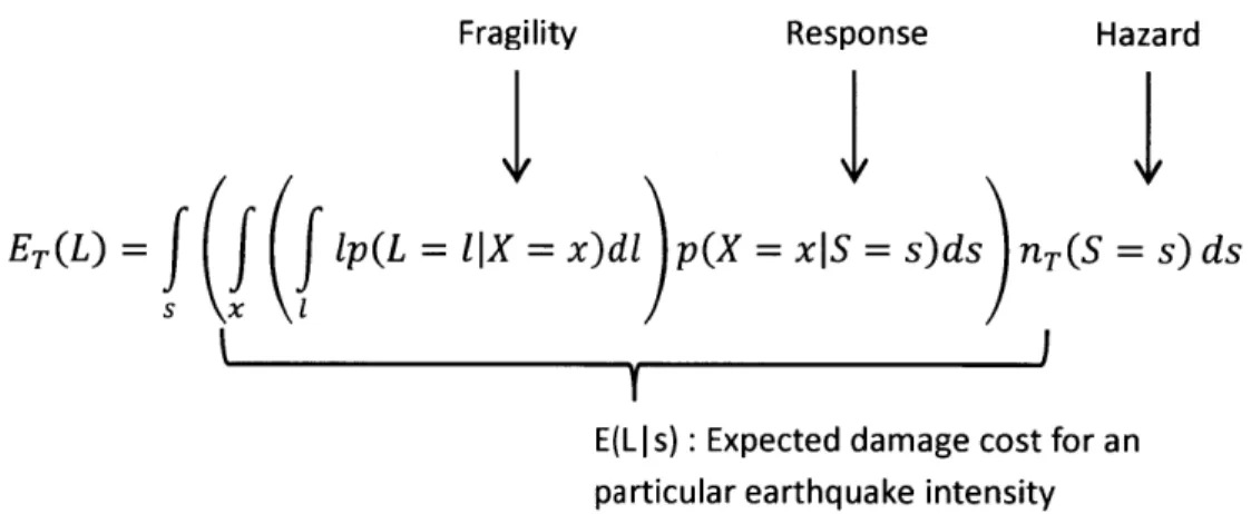
The total expected damage during a period of time T is an example of an overall seismic performance metric and is computed as:

Fragility ErL) = fff1p(L= s (x ( Response

I~

= s)ds) Hazard n IS nT (S = s) ds

T

E(LIs) : Expected damage cost for an particular earthquake intensity

Net present value of damage cost over y years: Ey(L) = EA(L) 1-ry

Other measures of seismic performance can be obtained in a similar way.

p(L=l I X=x) Fragility Function: Probability density of a damage L due to a response X=x j p(X=x IS=s) x Response Function: Probability density of a response X to a seismic event of intensity S=s Sn'(S=S) s Hazard Function: Frequency density of a seismic event of intensity S=s

Figure 2: Probabilistic functions involved in the overall seismic performance assessment.

4.3 Computation Procedure

To facilitate the computation of the total expected loss for a structure over a period of time, a model capable of time history response analysis must first be set up. Numerous software packages are available, and the level of complexity of the model greatly influences the time required to

1|X

= x)dl) p(X = xiS

(29)

perform the analysis. Once a model is developed, a set of ground motion records is then selected. How to pick an appropriate set of earthquakes is a much debated issue, and existing implementations of PEER's methodology recommend at least 50 ground motion records. This procedure is illustrated in Figure 3.

p(L=IIX=x) n(S=S)l

S

Building Ground motion \

model records Component Seismic hazard

loss distribution function

Figure 3: Model and data needed required for overall seismic performance assessment The following page illustrates how the above entities are combined in the PEER methodology; The relevant range of earthquake intensity is first discretized. Next, the structural response distribution is evaluated for each earthquake intensity value. To do this, each ground motion record is scaled to the appropriate earthquake intensity, applied to the structural model and the response is obtained through time-history analysis. Next, the response distribution function for the considered earthquake intensity is built from these results. This operation is repeated for each earthquake intensity. Once the response distribution is developed, the total expected loss can be computed by numerically integrating the different probabilistic functions.

(30)

modal analysis

(Tb, b)

for each earthquake intensity value si:

for each ground motion record

scale so that Sb =S

Sb denotes the intensity measure

S for a structure of class (Tb, (b)

compute add sample to p(X=xSb=si)

response distribution x ~ x p(X=xISb=si) p(X=x|Sb=si) - fit distribution 060 x p(X=x|Sb=s) s si combine p(X=xISb=s) distributions x X X X /p(L=IIX=x) p(X=xISb=s) nT(Sb=s) integrate ~E(L)= 1 dl dx ds xs s xI

(31)

5.0 CHALLENGES IN IMPLEMENTATION

One of the biggest challenges in implementation of the PEER methodology is the amount of time it takes to run analysis. Non-linear analyses of earthquake response are computationally expensive. If linear analyses could be substituted for non-linear, overall seismic performance metrics could be developed more rapidly and earlier in the design process.

Although linear and non-linear methods produce differences (more pronounced as the magnitude of earthquakes increase) such differences may not be significant when the values are used in a probabilistic performance assessment with other sources of uncertainty. Additionally, when considering the Probabilistic total cumulative damage over the lifetime of a building, it is reasonable to conclude that small to moderate events contribute significantly more than extreme events.

This thesis attempts to show that linear analysis is a valid substitute for non-linear analysis for the purposes of the PEER methodology.

(32)

(33)

6.0 MODEL

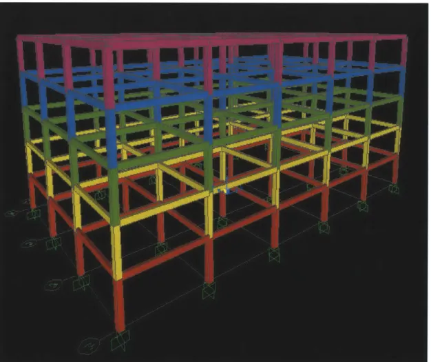
For the purposes of this thesis, a structural model of a fictitious 5-story reinforced concrete building was developed in SAP2000. The building has 5 bays in the "x" direction and 3 bays in the "y" direction. All bays were 30ft and inter-story heights were 12ft. A graphical

representation of the building is shown in Figure 5. Each floor has been assigned a different color for clarity.

Figure 5: SAP 2000 building model

For simplicity, all columns are of the same dimensions and all beams are of the same dimensions. Columns are 22x22 inches square with 3 #11 rebar running longitudinally along

(34)

each face. Beams are 20 inches deep and 10 inches wide with 4 #8 rebar running longitudinally along the top and bottom faces. A graphical representation of these elements are in Figure 6 and Figure 7, respectively.

(35)

[

wpauW

-ei"am. l s gIBEAMS r

damae inthe uildng fr nn-liear nalyis, ings insdaccgralnskce ihFM2 36wr nrn ah bea

-oc tekagtender..t~a

R Rectn.ft Ciis---- --

---teena _canm r na3iglaV'en d rg 1 _*am Figur 7: Beam details*Fa 1

(36)

(37)

7.0 ANALYSIS RESULTS

For the purposes of analysis, inter-story drift was analyzed.

7.1 Linear Comparison of scaled earthquakes

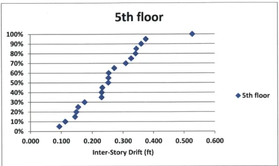
First, to illustrate that different earthquakes with the same peak ground acceleration (PGA) can induce very different responses in the same structure, the structural model was subject to a variety of earthquake time histories all scaled to a PGA of .1g. As expected, the response of the building was different for each earthquake. Tabulated results can be found in the appendix of this report in Table 2. Figure 8, Figure 9 and Figure 10 show the inter-story drifts.

1st floor

100% _$ 90% $ 80% 70% -60% -50% %1st floor 20% -10% 0% 0.000 0.010 0.020 0.030 0.040 Inter-Story Drift (ft)

(38)

5th floor

100% -90% -80% 70% -60% 50% 40% _{*5th floor} 30% -20% 10% 0% 0.000 0.100 0.200 0.300 0.400 0.500 0.600 Inter-Story Drift (ft)

Figure 9: 5th Floor Inter-story drifts for 20 earthquakes scaled to .lg

1st floor 4.0 m 3.0 U" - 2.0 -ist floor

0 -- per. Mov. Avg. (1st floor)

0.0

-ans g mms N msmaM sM ans

cc

V aI 0 0 i01010 I0 0 I0V

Inter-Story Drift (ft)

Figure 10: Inter-story drifts for 20 earthquakes scaled to .lg The distribution is similar to log-normal.

(39)

7.2 Comparison of Linear and Non-Linear Analysis

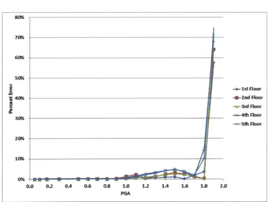
Next, the time history of the Loma Prieta earthquake on 10/18/89 as measured at the Agnews State Hospital was scaled to 19 different magnitudes and both linear and non-linear

analyses were performed.

The error (defined in the equation below) was then plotted (See Figure 11). It should be noted that the model building was over designed requiring excessively high PGA's to induce inelastic behavior. However, the general trend in the results is believed valid. i.e. Reducing the strength of the model should produce the same trend with the % error increasing at a lower PGA.

Error = I Inter - story driftnon-inear - Inter - story driftinear|

Inter - story driftnon-inear

701V 60% 50M +1st Floor S4C% -*-Znd Floor ,r3r Floor --8Floor -a-4th floor -5Sth Floor 20% love 0% 0.0 0.2 OA 0.6 0.8 1.0 1.2 1A 1.6 18 2.0 PFA

(40)

It is clear from these results that linear and non-linear results strongly agree before and after plastic hinges form. It is not until the structure is close to failure that behavior diverges.

7.3 Cost

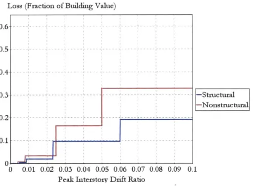
To compare life-time cost of repair estimates for linear and non-linear analysis results, the fragility function and annual occurrence density shown below were applied to the

inter-story drift ratios from analysis. Three locations were considered: Los Angeles, CA, San Francisco, CA and Anchorage, AK.

Loss (Fraction of Building Value)

0.4

0.3 - - - -Structural

-Nonstructural

0

0 0.01 0.02 0.03 0.04 0.05 0.06 0.07 0.08 0.09 0.1

Peak Interstory Drift Ratio

Figure 12: Fragility function for commercial offices designed to moderate code requirements

s -

a(2s + b)

(41)

Los Angeles, CA: San Francisco, CA: Anchorage, AK:

a = 0.7346 a = 0.7179 a = 0.487

b = 1.869 b = 3.202 b = 0.6462

c = 0.625 c = 0.9744 c = 0.2735

Applying these parameters and assuming a building life of 100 years and a 3% interest rate and an equal value for each floor of the building (20% of the total building value), the estimated cost of structural damage to the structure over the lifetime of the building is summarized in Table 1.

Table 1: Cost of Damage over lifetime of building (% of original building value)

Los Angeles San Francisco Anchorage

Linear Non-Linear

yearly lifetime yearly lifetime % error

7% 236% 7% 237% 0.17%

4% 141% 4% 142% 0.19%

12% 376% 12% 376% 0.13%

This clearly demonstrates that linear and non-linear analysis produce nearly identical results (less than 1% error). It should be noted that the model used in this study required excessive

inter-story drift before hinges formed and non-linear behavior occurred. For weaker

buildings it is expected that there will be a greater difference in cost. However, because the stronger earthquakes are weighted so lightly in this methodology it is expected these

differences will still be within an acceptable margin of error.

7.4 Analysis time

The non-linear analyses took over 700-times longer than linear analysis:

The average time for non-linear analysis was 51 minutes while the average time for linear analysis was 6 seconds.

(42)

(43)

8.0 CONCLUSIONS AND RECOMMENDATIONS

These results clearly show that linear analysis of earthquakes with smaller magnitudes yield results very similar to those produced with non-linear analysis. Considering the number of analyses required when applying the PEER methodology and the potential times savings, it makes good engineering sense to use linear analysis.

There is a potential for significant time savings should linear analysis be substituted for excessively accurate non-linear.

(44)

(45)

9.0 REFERENCES

ASCE-31 (2003). Seismic Evaluation of Existing Buildings. ASCE 7-05(2003). Minimum Design Loads for Buildings. ASCE-41 (2006). Seismic Rehabilitation of Existing Buildings.

Aslani, H., E. Miranda. 2005. Probability-based seismic response analysis. Engineering Structures 27, 1151-1163.

Celikbas, Ayse. 1999. Economics of damage controlled seismic design. S.M., Massachusetts Institute of Technology, Dept. of Civil and Environmental Engineering.

Connor, J. J. 2003. Introduction to structural motion control. 1t ed. Upper Saddle River, New Jersey 07458: Prentice hall, Pearson Education, Incc.

Connor, J. J., A. Wada, M. Iwata, and Y. J. Huang. 1997. Damage-controlled structures. 1: Preliminary design methodology for seismically active regions. Journal of Structural Engineering 123, (4) (April 1997): 423-31

FEMA-445 (2006). Next-Generation Performance-Based Seismic Guidelines - Program Plan for New and Existing Buidlings.

Iwata, M. 1994. Damage level control design. 109, (1352): 42-4

Krawinkler, H., F. Zareian, R. Medina, and L. Ibarra. 2005. Decision support for conceptual performance-based design. Wiley InterScience (www.interscience.wiley.com), DOI: 10.1002/eqe.536

Krawinkler, H., F. Zareian, R. Medina, and L. Ibarra. 2006. Decision support for conceptual performance-based design. Earthquake Engineering and Structural Dynamics 35, 115-133 Moehle, Stojadinovic, Der Kiureghian and Yang (2005). An Application of PEER Performance-Based Earthquake Engineering Methodology. Pacific Earthquake Engineering Reasearch Center

(46)

(47)

10.0 APPENDICES

Table 2: Inter-story drift results for 20 earthquakes scaled to PGA=.lg

I ~ d d d 6 d o

£111m

I!

I

_{I I I iI}

_II

(48)

Table 3: Inter-story drift error results for Loma Prieta 10/18/89 Earthquake as measured at Agnews State Hospital scaled to 19 PGAs

ec In I

w

a

1laMIE

# a'0il0

il

Oini

INNE

I!Ij

MillE

I d v i 1 d a t

I4

4 tit 1I I 11111111111111

(49)

Table 4: Analysis Time r M M IF qv GA In 04 N N%

li

illli

il

toIIII

3i

El

tillllil111

91 i

11. il

111 111 1

(50)

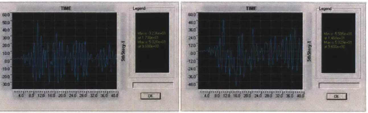
Figure 13: Screen Shots of 5th Story inter-story displacement for linear (left) and non-linear (right) analysis

Figure 14: Screen shot of the time history of 5 inter-story displacements - Clearly the fundamental mode is being excited as all floors remain in phase.

(51)

Table 5: Error in inter-story drift for Loma Prieta 10/18/89 Earthquake as measured at Agnews State Hospital scaled to PGA = .05 (No hinges formed)

MIl

I

a.

(52)

Table 6: Error in inter-story drift for Loma Prieta 10/18/89 Earthquake as measured at Agnews State Hospital scaled to PGA = .lg (No hinges Formed)

Il

II

il

(53)

Table 7: Table 5: Error in inter-story drift for Loma Prieta 10/18/89 Earthquake as measured at Agnews State Hospital scaled to PGA = .172g (No hinges Formed)

'I"

11

A

11

(54)

lii

ill-H

A

1

1 i

iII

dI

(55)

n mI

I

hi

Il

mi

II

I|

(56)

Ji.

(57)

Table 11: Table 5: Error in inter-story drift for Loma Prieta 10/18/89 Earthquake as measured at Agnews State Hospital scaled to PGA = .7g (No hinges Formed)

1 g

11

(58)

Table 12: Table 5: Error in inter-story drift for Loma Prieta 10/18/89 Earthquake as measured at Agnews State Hospital scaled to PGA = .8g (No hinges Formed)

O!

il

Iul

(59)

U~

01

4k

Igo

Figure 15: Hinges formed and error in inter-story drift for Loma Prieta 10/18/89 Earthquake as measured at Agnews State Hospital scaled to PGA=.9g

(60)

6I

Figure 16: Hinges formed and error in inter-story drift for Loma Prieta 10/18/89 Earthquake as measured at Agnews State Hospital scaled to PGA=1.0g

(61)

c

aI

GL

Ri -? / / x R M ll!! M!l~l v NT M z x+ a

(62)

Xi"

71

(63)

-xiiITI

E E R

HH

&X X

(64)

I

IA

li1

(65)

A1lis

4N

_XI

EI

1C1

(66)

Ii

I

II

j

I

Figure 22: Hinges formed and error in inter-story drift for Loma Prieta 10/18/89 as measured at Agnews State Hospital scaled to PGA=1.6g

5 I

I

a

I

'WI

ii

II

I

I Earthquake

31 §11

(67)

.,

(68)

6I

IM

Xi

11

b

(69)

c

H

4 & 6

tEByn me

/ i!

x

x+=s

5

Fiue2:Hne4omdaderri ne-tr rf o o aPit 01/9Erhuk

(70)

Figure 26: Time history for San Fernando 02/09/7114:00 LAHollywood Stor Lot earthquake Imperial Valley 10/15/79 23:16 Chihuahua

0.300 g 0.200 g 0.100 g -0.000 g - - - --0.100 g 0.200 g --0.300 g 0 10 20 30 40 50 Time (Seconds)

Figure 27: Time history for Imperial Valley 10/15/79 23:16 Chihuahua earthquake San Fernando 02/09/7114:00 LA Hollywood Stor Lot

0.003 g 0.002 g 0.001 g -0.000 g -di. - --0.001 g --- - - -- - - - - --0.002 g -0.003 g 0 5 10 15 20 25 30 Time (Seconds)

(71)

Figure 28: Time history for Imperial Valley 10/15/79 23:16 Compuertas earthquake

Figure 29: Time history for Imperial Valley 10/15/79 23:16 El Centro Array #12 earthquake

Imperial Valley 10/15/79 23:16 Compuertas

0.200 g 0.150 g 0.100 g 0.050 g -0.000 g 0.050 g --0.100 g --0.150 g -0.200 g 0 5 10 15 20 25 30 35 40 Time (Seconds)

Imperial Valley 10/15/79 23:16 El Centro Array #12

0.150 g 0.100 g -m 0.050 g -0.000 g --0.050 g --0.100 g -0.150 g 0 10 20 30 40 50 Time (Seconds)

(72)

Figure 30: Time history for Imperial Valley 10/15/79 23:16 El Centro Array #13 earthquake Imperial Valley 10/15/79 23:16 Plaster City

0.050 g -0.040 g - 0.030 g 0.020 g 0.010 g 0.000 g --0.010 g 0.020 g 0.030 g 0.040 g --0.050 g 0 5 10 15 20 Time (Seconds)

Figure 31: Time history for Imperial Valley 10/15/79 23:16 Plaster City earthquake Imperial Valley 10/15/79 23:16 El Centro Array #13

0.150 g 0.100 g 0.050 g -0.000 g -liIAdp -0.050 g--0.100 g -0.150 g 0 10 20 30 40 50 Time (Seconds)

(73)

Superstition Hills 11/24/87 13:16 EICentro Imp Co Center 0.400 _g 0.300 _g 0.200 g 0.100 g -0.000 g -- A k.fhAsatot" -0.200 g --0.300 g -0.400 g -0.400 g 0 10 20 30 40 50 Time (Seconds)

Figure 32: Time history for Superstition Hills 11/24/87 13:16 EICentro Imp Co Center earthquake

Superstition Hills 11/24/87 13:16 Wildlife Liquefaction Array 0.400 g 0.300 g 0.200 g 0.100 g 0.000 g -ALA A AL

0.100 g -W v w wwwi w -0.200 g -0.300 g -0.400 g 0 10 20 30 40 50 Time (Seconds)

Figure 33: Time history for Superstition Hills 11/24/87 13:16 Wildlife Liquefaction Array earthquake

(74)

Figure 34: Time history for Loma Prieta 10/18/89 00:05 Agnews State Hospital earthquake Loma Prieta 10/18/89 00:05 Anderson Dam

Downstream 0.300 _g 0.200 _g 0.100 g 0.000 g --0.100 g--0. 200 g -0.300 g 0 10 20 30 40 50 Time (Seconds)

Figure 35: Time history for Loma Prieta 10/18/89 00:05 Anderson Dam Downstream earthquake

Figure

Loma Prieta 10/18/89 00:05 Agnews State Hospital

0.200 g 0.150 g 0.100 g 0.050 g 0.000 g --0.050 g --0.100 g -0.150 g -0.200 g 0 10 20 30 40 50 Time (Seconds)

(75)

Figure 36: Time history

Figure 37: Time history for

for Loma Prieta 10/18/89 00:05 Coyote Lake Dam Downstream earthquake

Loma Prieta 10/18/89 00:05 Halls Valley earthquake

Figure

Loma Prieta 10/18/89 00:05 Coyote Lake Dam Downstream 0.200 _g 0.150 _g 0.100 _g 0.050 g 0.000 g 0.050 g --0.100 g -0.150 g -0.200 g 0 10 20 30 40 50 Time (Seconds)

Loma Prieta 10/18/89 00:05 Halls Valley

0.150 g 0.100 _g 0.050 g 0.000 g 0.050 g --0.100 g -0.150 g 0 10 20 30 40 50 Time (Seconds)

(76)

Figure 38: Time history for Loma Prieta 10/18/89 00:05 Hollister South & Pine earthquake

Figure 39: Time history for Loma Prieta 10/18/89 00:05 Hollister Diff Array earthquake Loma Prieta 10/18/89 00:05 Hollister South & Pine

0.500 g -0.400 g -0.300 g -0.200 g 0.100 g 0.000 g -0.100 g -0.200 g --0.300 g -0.400 g -0.500 g-0 10 20 30 40 50 60 70 Time (Seconds)

(77)

Figure 40: Time history for Loma Prieta 10/18/89 00:05 Waho earthquake Northridge 01/17/94 12:31 LA - Baldwin Hills

0.300 g 0.250 g 0.200 g 0.150 g 0.100 g -0.050 g -0.000 g --0.050 g -0.100 -0.150 g--0.200 g -0.250 g 0 10 20 30 40 50 Time (Seconds)

(78)

Figure 42: Time history for Northridge 1/17/94 12:31 LA - Centinela earthquake

Figure 43: Time history for Northridge 1/17/94 12:31 LA -Hollywood Storage FF earthquake

Northridge 1/17/94 12:31 LA - Centinela 0.600 g 0.400 g 0.200 g 0.000 g --0.200 g -0.400 g -0.600 g 0 5 10 15 20 25 30 35 Time (Seconds)

Northridge 1/17/94 12:31 LA -Hollywood Storage FF 0.300 g 0.200 g 0.100 g -0.000 _g --0.100 g --0.200 g -0.300 g 0 10 20 30 40 50 Time (Seconds)

(79)

Figure 44: Time history for Northridge 1/17/94 23:31 Lake Hughes #1 - Fire Station #78 earthquake C 0.100 g -0.080 g -0.060 g 0.040 g -0.020 g 0.000 g --0.020 g --0.040 g --0.060 g -0.080 g -0.100 g 0 5 10 15 20 25 30 35 Time (Seconds)

Figure 45: Time history for Northridge 1/17/94 23:31 earthquake

(80)

Table 13: Lifetime cost of damage assessment - Los Angeles, CA a .7346 b 1.869 c 0.625 PGA LOS ANGELES n(s) = -gl(s)/ds = a * (2's + b) / (s's + b's + c)A2 Total yearly cost 7.484% LINEAR ANALYSIS 0.05 g t NON-LINEAR ANALYSIS

Floor % cost PIDR ROUND LOSS COST % cost PIDR ROUND LOSS COST

1st 0.2 0 0.001 0 0 0.2 0 0.001 0 0

2nd 0.2 0 0.003 0 0 0.2 0 0.003 0 0

3rd 0.2 0 0.006 0.01 0 0.2 0 0.006 0.01 0

4th 0.2 0 0.008 0.01 0 0.2 0 0.008 0.01 0

5th 0.2 0 0.01 0.02 0 n(s) yearly cost 0.2 0 0.01 0.02 0 n(s) yearly cost Total 0.01 0.28 0.17% Total 0.01 0.28 0.17%

PGA 0.1 g

% cost PIDR ROUND LOSS COST % cost PIDR ROUND LOSS COST 1st 0.2 0 0.002 0 0 0.2 0 0.002 0 0

2nd 0.2 0 0.006 0.01 0 0.2 0 0.006 0.01 0

3rd 0.2 0 0.011 0.02 0 0.2 0 0.011 0.02 0

4th 0.2 0 0.016 0.02 0 0.2 0 0.016 0.02 0

5th 0.2 0 0.02 0.02 0 n(s) yearly cost 0.2 0 0.02 0.02 0 n(s) yearly cost Total 0.01 0.14 0.18% Total 0.01 0.14 0.18%

PGA 0.17 g

% cost PIDR ROUND LOSS COST % cost PIDR ROUND LOSS COST

1st 0.2 0 0.003 0 0 0.2 0 0.003 0 0

2nd 0.2 0 0.01 0.02 0 0.2 0 0.01 0.02 0

3rd 0.2 0 0.019 0.02 0 0.2 0 0.019 0.02 0

4th 0.2 0 0.027 0.1 0.02 0.2 0 0.027 0.1 0.02

5th 0.2 0 0.034 0.1 0.02 n(s) yearly cost 0.2 0 0.034 0.1 0.02 n(s) yearly cost Total 0.05 0.17 0.78% Total 0.05 0.17 0.78%

PGA 0.3 g

1st 0.2 0 0.005 0.01 0 0.2 0 0.005 0.01 0

2nd 0.2 0 0.016 0.02 0 0.2 0 0.016 0.02 0

3rd 0.2 0 0.032 0.1 0.02 0.2 0 0.032 0.1 0.02

4th 0.2 0 0.047 0.1 0.02 0.2 0 0.047 0.1 0.02

5th 0.2 0.1 0.059 0.1 0.02 n(s) yearly cost 0.2 0.1 0.059 0.1 0.02 n(s) yearly cost Total 0.06 0.18 1.13% Total 0.06 0.18 1.13%

PGA 0.5 g

1st 0.2 0 0.007 0.01 0 0.2 0 0.007 0.01 0

2nd 0.2 0 0.027 0.1 0.02 0.2 0 0.027 0.1 0.02

3rd 0.2 0.1 0.054 0.1 0.02 0.2 0.1 0.054 0.1 0.02

4th 0.2 0.1 0.078 0.19 0.04 0.2 0.1 0.078 0.19 0.04

5th 0.2 0.1 0.097 0.19 0.04 n(s) yearly cost 0.2 0.1 0.097 0.19 0.04 n(s) yearly cost Total 0.12 0.1 1.11% Total 0.12 0.1 1.11%

Total yearly cost

Applicability of linear analysis in probabilistic estimation of seismic building damage to reinforced-concrete structures

Applicability of Linear Analysis in Probabilistic Estimation of

Seismic Building Damage to Reinforced-Concrete Structures

ARCHIVES

Applicability of Linear Analysis in Probabilistic Estimation of

Seismic Building Damage to Reinforced-Concrete Structures

To Yuko:

{±1~

MIT

4E

MI

d

liX

I~

T

1|X

[

wpauW

1st floor

5th floor

s -

a(2s + b)

£111m

I!

I

I I I iI

II

ec In I

w

a

# a'0il0

il

Oini

INNE

I!Ij

MillE

I4

li

il

toIIII

3i

El

tillllil111

91

i

11.

il

111 111 1

MIl

I

Il

II

il

'I"

A

11

lii

ill-H

A

1

1

i

iII

dI

n mI

I

hi

Il

II

I|

Ji.

1

g

11

il

Iul

U~

01

Igo

6I

_{I I I iI}

_II