HAL Id: hal-01491099
https://hal-amu.archives-ouvertes.fr/hal-01491099
Submitted on 2 May 2018HAL is a multi-disciplinary open access archive for the deposit and dissemination of sci-entific research documents, whether they are pub-lished or not. The documents may come from teaching and research institutions in France or abroad, or from public or private research centers.
L’archive ouverte pluridisciplinaire HAL, est destinée au dépôt et à la diffusion de documents scientifiques de niveau recherche, publiés ou non, émanant des établissements d’enseignement et de recherche français ou étrangers, des laboratoires publics ou privés.
groundwater pollutants with BIOSCREEN-AT-ISO
Patrick Höhener, Zhi Li, Maxime Julien, Pierrick Nun, Richard J. Robins,
Gérald S. Remaud
To cite this version:
Patrick Höhener, Zhi Li, Maxime Julien, Pierrick Nun, Richard J. Robins, et al.. Simulating compound-specific isotope ratios in plumes of groundwater pollutants with BIOSCREEN-AT-ISO. Groundwater, Wiley, 2017, 55 (2), pp.261-267. �10.1111/gwat.12472�. �hal-01491099�
Simulating stable isotope ratios in plumes of groundwater pollutants with
BIOSCREEN-AT-ISO
Patrick Höhener1*, Zhi M. Li1, Maxime Julien2, Pierrick Nun2, Richard J. Robins2, Gérald
S. Remaud2
1
Aix Marseille Univ,–CNRS UMR 7376, Laboratoire Chimie Environnement, 3 place Victor Hugo, F-13331 Marseille, France.
2
Nantes University, CNRS UMR 6230, EBSI team, CEISAM, 2 rue de la Houssinière, F-44322 Nantes, France.
*Corresponding author: Patrick Höhener, Phone: ++33 4 13 55 10 34; Fax ++33 4 13 55 10 60; e-mail: patrick.hohener@univ-amu.fr
Revised version, GW20160413-0085
Abstract
1
BIOSCREEN is a well-known simple tool for evaluating the transport of dissolved 2
contaminants in groundwater, ideal for rapid screening and teaching. This work extends the 3
BIOSCREEN model for the calculation of stable isotope ratios in contaminants. A three-4
dimensional exact solution of the reactive transport from a patch source, accounting for 5
fractionation by first-order decay and/or sorption, is used. The results match those from a 6
previously published isotope model but are much simpler to obtain. Two different isotopes 7
may be computed, and dual isotope plots can be viewed. The dual isotope assessment is a 8
rapidly emerging new approach for identifying process mechanisms in aquifers. Furthermore, 9
deviations of isotope ratios at specific reactive positions with respect to “bulk” ratios in the 10
whole compound can be simulated. This model is named BIOSCREEN-AT-ISO and will be 11
downloadable from the journal homepage. 12
13
Article Impact Statement
14
This BIOSCREEN-AT decision support system can compute compound- and position-15
specific stable isotope ratios in groundwater pollutant plumes. 16
17
Keywords
18
Reactive transport, saturated zone, contaminated sites, natural attenuation, stable isotopes 19
Introduction
20The BIOSCREEN model had been developed by the US EPA in 1996 (Newell et al. 1996) as a 21
user-friendly simulation tool for the evaluation of the transport of dissolved contaminants in 22
groundwater. Under the name of BIOSCREEN-AT, an improved version based on the exact 23
analytical solution for reactive transport from a patch source in 3 dimensions was later published 24
(Karanovic et al. 2007) and distributed as an MS EXCEL-based spreadsheet. Within the last 15 25
years, considerable progress has been made in the analysis of isotope ratios in dissolved 26
groundwater pollutants. Compound-specific isotope analysis (CSIA) of either 13C, 2H, or 15N can 27
be made using isotope ratio monitoring by Mass Spectrometry (irm-MS) (Hofstetter and Berg 28
2007; Elsner 2010; Thullner et al. 2012). This method is able to realize multi-element analyses 29
using a small amount of sample and to determine isotope ratios of mixtures components using 30
Gas Chromatography (GC) or High Performance Liquid Chromatography (HPLC) coupling. The 31
main inconvenient of this method is that it only allows determining the average over the whole 32
molecule isotopic composition, missing the intramolecular distribution of heavy isotopes in the 33
studied compounds. In this context, different methods have been developed in order to perform 34
Position-Specific Isotope Analysis (PSIA). The isotope ratio measurement by 13C Nuclear 35
Magnetic Resonance Spectrometry (irm-13C NMR) is a recently developed technique capable of 36
determining the isotopic composition of each carbon position of a large panel of molecules 37
(Caytan et al. 2007). In a previous study, irm-13C NMR has recently proven its interest in the 38
determination of origin of contaminants (Julien et al. 2016) and the study of their remediation 39
(Julien et al. 2015a+b). 40
Changes in isotope ratios during reactive transport are indicative of reactive processes: bond-41
breaking processes can cause a large isotope fractionation at the position of the initial bond 42
cleavage, often leading to an enrichment of the remaining non-degraded pollutant.. Smaller 43
secondary isotope fractionation at t sites adjacent to a reactive position can also occur. Also, 44
when the transformation products of pollutants are also components of the primary pollutants in 45
the contamination source, isotope ratio can be used to differentiate the origins of chemicals and 46
provide actual description of reactive processes. Thus, US EPA recommended the use of CSIA to 47
access biodegradation processes and to identify the source of organic groundwater contaminants 48
(Hunkeler et al. 2008). CSIA has been largely applied to study natural attenuation processes in 49
contaminated field investigation like discussed in three critical review articles (Meckenstock et 50
al. 2004; Schmidt et al. 2004; Elsner 2010). To our knowledge, PSIA has not been applied in 51
field investigation but it represents a promoting trend of isotope fractionation pattern for the 52
study of natural attenuation processes in contaminated groundwater. 53
Equilibrium sorption can also create small to intermediate isotope fractionation at certain 54
positions of molecules, but unfortunately the effect also causes in most cases an enrichment of 55
the remaining pollutant (Kopinke et al. 2005; Höhener and Yu 2012), which could be wrongly 56
interpreted as an effect of degradation. In contrast, the physical dilution of compounds should a 57
priori not change isotope ratios (Elsner 2010). In combination, these isotope fractionations can 58
impact on the bulk (average over the whole molecule) isotope ratios observed, but position 59
specific fractionations are inevitably diluted out when only CSIA is exploited. PSIA, in contrast, 60
gives access to the individual values. 61
Because of the high information content of isotope ratios in contaminants in groundwater plumes, 62
they are often measured to obtain a better understanding of natural attenuation processes. 63
Moreover, fractionation factors for a large number of bond-breaking reactions and for 64
equilibrium sorption are available (Aelion et al. 2010; Höhener and Yu 2012). 65
Analytical or numerical models for compound-specific isotope ratios in aquifer pollutants have 66
been developed. Höhener and Atteia (2010) showed with analytical models on MAPLE 67
worksheets that only the exact analytical solution in BIOSCREEN-AT gives correct isotope 68
ratios at lateral plume margins. However, all current isotope models are quite demanding in 69
operational skills and partly also in CPU time and therefore have not been widely exploited. 70
The present work here combines the know-how of isotope evolution from the more complex 71
models with the well-known and user-friendly model BIOSCREEN-AT to propose a simple tool 72
predicting isotope ratios in groundwater as a function of time and space. The tool should compute 73
two different isotopes in each compound (e.g. 13C and 2H) in order to create the so-called dual-74
isotope plots (Vogt et al. 2016). These plots are very sensitive to different reaction mechanisms. 75
The overall goal is that a user can rapidly deduce whether their combined data on concentration 76
and isotope ratios prove unambiguously the degradation and/or sorption of the target pollutant in 77
the studied aquifer. 78
Analytical solution and its implementation
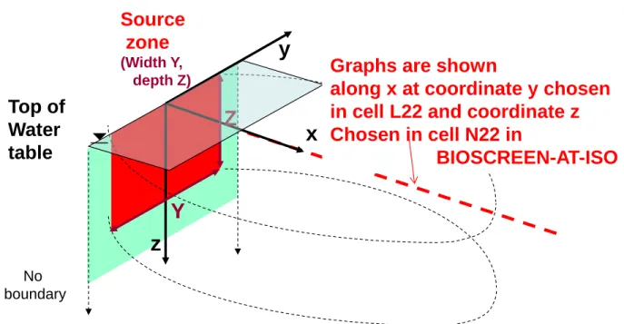
79The schematic representation of the pollution scenario in a homogeneous 3-dimensional aquifer 80
is shown in Figure 1. The aquifer is semi-infinite in the x direction, and infinite in the y and z 81
directions. Reactive transport is modeled with the advection-dispersion equation given for the x-82
y-z space as in equation (1), under the following assumptions: groundwater flow is steady and 83
uni-directional along the x-axis; material properties are homogeneous; partitioning between 84
dissolved and sorbed phases is instantaneous and reversible; neither gas phases nor volatilization 85
from groundwater is modeled; the solute undergoes degradation following first-order kinetics, but 86
only in the dissolved phase (which is realistic for microorganisms which degrade dissolved 87
pollutants at low environmental concentrations). 88
C x C v z C v y C v x C v t C Rf x y z 2 2 2 2 2 2 (1) 89
In Eq. (1), v is the unretarded groundwater flow velocity (m yr-1), x is longitudinal dispersivity
90
(m), y, and z are the transversal dispersivities in the y (horizontal), and z (vertical) direction
91
(m), is a first-order degradation rate (yr-1), and Rf is the retardation factor (see eq. (4)). We use
92
the exact solution of eq. (1) from Cleary and Ungs (1978) which is equation (2): 93 (2) 94 with 95 96 97 98 99
and where i stands for a specific isotope, is a first-order decay rate of the concentration in the 100
source, v’ = v/Rf,i, and C0,i is the (constant) concentration of isotope i in the source (mol L-1).
101
The use of the exact solution fixes problems associated with the first BIOSCREEN model which 102
was based on Domenico’s analytical solution. This issue was broadly discussed in several 103
publications (Guyonnet and Neville 2004; Srinivasan 2007; West et al. 2007). 104
For isotope modeling, we use the isotope approach (Hunkeler et al. 2009; Höhener and Atteia 105
2010) where each isotope is modeled separately. Light (l) and heavy (h) isotopes are modeled 106
using different caused by kinetic isotope fractionation during bond cleavage (fractionation 107
factor react), and using different Rf,i caused by equilibrium isotope effects by sorption
108
(fractionation factor sorption, eqns. 3-5,Höhener and Yu 2012).
109 l = (3a) 110 ) , , , , ( , 0 ) , , , (x yzt i ixy zt i
C
C
d
v
Z
z
erfc
v
Z
z
erfc
v
Y
y
erfc
v
Y
y
erfc
v
x
R
v
x
t
v
x
y y y y x i f i t x t z y x i
'
2
'
2
'
2
5
.
0
'
2
5
.
0
'
4
exp
1
'
exp
'
8
2 , 0 5 . 1 ) , , , , (h = react (3a) 111 OC OC b f l K f n R 1 (4a) 112 sorption OC OC b f h K f n R 1 (4b) 113
0
0 0 C /1 R C l (5a) 114
0
0 0 0 C R /1 R C h (5b) 115Here, b is the soil bulk density (kg L-1), n is effective porosity, KOC is the partitioning coefficient
116
of the contaminant between organic carbon and water (L kg-1), fOC is the unitless fraction of
117
organic carbon of the aquifer solids, and R0 is the initial (constant) isotope ratio of the
118
contaminant in the source. Equations 3 and 4 create different transport behavior of light and 119
heavy isotopes, which finally lead to changes in the isotope ratios. 120
These isotope ratios in delta notation (in ‰) are finally obtained by equation (6): 121 1000 1 ) , , , ( ) , , , ( ) , , , ( standard t z y x l t z y x h t z y x R C C (6) 122
where Rstandard is the isotope ratio of the international standard for the element of interest.
123
For the purpose of the assessment of degradation, equation (7), which computes the percent of 124
degradation B (%) compared to overall concentration decrease in the contaminant, was 125
incorporated into the model: 126 100 1000 1000 1 (%) / 1000 reaction source B (7) 127
B (%) is mainly caused by biotic reaction, but at some sites also abiotic reactions were found to 128
fractionate isotopes. The equation 7 is only valid when the change in isotope ratios is uniquely 129
caused by reaction. In cases where sorption fractionates isotopes, the B (%) will be wrong. This is 130
illustrated in the spreadsheet because the model gives also the true B (%) obtained from modeling 131
a sorption-affected tracer and equation (8). 132
source tracer tracer source compound compound trueC
C
C
C
B
, ,1
100
%
(8) 133Here, Ctracer is a simulated concentration of a sorbing tracer affected by Rf. The equations were
134
implemented on a spreadsheet (MS EXCEL, version 2010). The integration of the factors of 135
equation (1) is made in 100 steps of d. In order to test the exactness of the approach 136
implemented in EXCEL, the results were compared to numerical integrations made by MAPLE 137
(version 13, Waterloo Maple Inc, Waterloo, Canada) using the Maple worksheet from Höhener 138
and Atteia (2010) with the exact solution of Wexler (1992). 139
Example calculations
140The presented example here is for methyl tert-butyl ether (MTBE). Fractionation factors of 13C 141
and 2H during aerobic degradation were chosen as similar to those found in laboratory 142
experiments (Rosell et al. 2007). MTBE has an intra-molecular variation in 13C isotope ratio, with 143
the methyl group (in the NMR spectrum position 2 according to the chemical shift) being most 144
negative (Julien et al. 2016). Initial enzymatic attack will occur at this position, leading to the 145
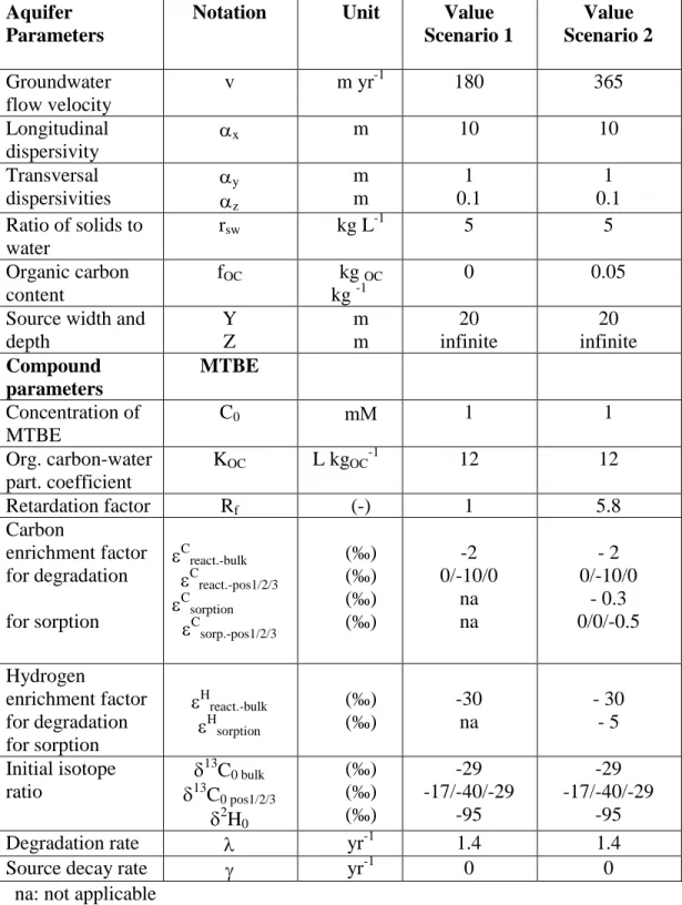
largest isotope fractionation at this C atom. Two scenarios were modeled (see Table 1 for model 146
parameters). Scenario 1 presents an old plume in groundwater with low flow velocity, without 147
any sorption, whereas scenario 2 is a young plume in a faster flowing groundwater where 148
sorption occurs and sorption fractionates the pollutant in addition to the fractionation by 149
degradation. Both scenarios were modeled with the present model (BIOSCREEN-AT-ISO) and 150
the MAPLE model (Höhener and Atteia 2010). The results are shown in Figures 2 and 3. 151
Figures 2a and 3a show that concentrations along the plume centerline both match exactly the 152
concentrations modeled by the MAPLE worksheet, indicating that the integration of time in the 153
EXCEL model in 100 steps is sufficiently accurate compared to an independent numerical 154
integration both for short and long times (2 and 50 years). The other subsets in Figures 2 and 3 155
show that both models also yield identical results for isotope ratios of 13C and of 2H. The 156
modeled curves along the plume centerline indicate that the isotope data enable a clear distinction 157
between scenario 1, wherein only degradation fractionates, and scenario 2, wherein sorption also 158
contributes to fractionation. The increases of the ratios are enhanced in scenario 2, especially at 159
the forerunning plume front. The explanation for this is that only at the fore-running front of 160
young plumes, there are sorption sites unoccupied by the contaminant, and therefore fractionation 161
can occur when the contaminant sorbs to these sites. Near the source, or everywhere in old 162
plumes, sorption sites are already occupied by contaminant, and no fractionation occurs anymore. 163
This had previously been predicted (Kopinke et al. 2005). Figures 2c and 3c show that the slope 164
in the dual isotope plots 2H vs 13C does not lie exactly on the approximation 165
H/C15 in both cases, and that the present model is a helpful tool to investigate why and how 166
such slopes change as a function of two fractionating processes and of dispersion. It had been 167
shown previously that dispersion must be taken into account for the interpretation of field isotope 168
data, even when dispersion itself does not create fractionation (Abe and Hunkeler 2006). Finally, 169
Figures 2b and 3b show in addition that, for the carbon isotope ratios, a position-specific isotope 170
measurement of 13C would enhance even more the discriminatory power of the isotope 171
approach, since the 13C in the reactive position 2 increases by up to 10‰, whereas the bulk 13C 172
increases only by 2‰. Once progress is made in the purification of samples in order to perform 173
PSIA by NMR (Julien et al. 2015) in real-world groundwater, our model is operational for data 174 interpretation. 175
Conclusions
176To sum up, the BIOSCREEN-AT-ISO model with stable isotopes is validated in this work and 177
can serve in future as a tool for isotope geochemists for the assessment of natural attenuation of 178
dissolved groundwater pollutants during reactive transport. The BIOSCREEN-AT format was 179
chosen because it gained popularity in the community of groundwater remediation and proved to 180
be useful for rapid assessment and teaching. The study of field processes using compound-181
specific isotope analysis is recommended by US EPA which published guidelines for isotope data 182
interpretations (Hunkeler et al. 2008). Field data of concentrations and isotope ratios are easily 183
assessed with the model, and the contribution of biodegradation to natural attenuation can be 184
quantified at any point in the aquifer. The model predicts dual isotope evolutions in space and 185
time and reinforces interpretations of degradation mechanisms (Vogt et al. 2016). The model is 186
an ideal complement to more sophisticated numerical models: this analytical model is free of 187
numerical dispersion and can be used to validate results from numerical codes for homogeneous 188
cases. More sophisticated numerical approaches would need very time-consuming tailor-made 189
modeling and maybe development of codes, while the use of a spreadsheet model like 190
BIOSCREE-AT-ISO can simulate in some hours a three-dimensional field case and can check 191
whether an investment in more complex models is worthwhile. The limitations of this model 192
compared to numerical approaches are: 1) it is only valid only in homogeneous systems; 2) only 193
for constant or experimentally decaying sources; 3) only for linear sorption isotherms; and 4) 194
only for stable isotopes of C, H, N, and O, but not for Cl which behaves differently (Hunkeler et 195
al. 2009). The BIOSCREEN-AT-ISO is a Microsoft EXCEL spreadsheet compatible with 196
versions 2010 or later and can be downloaded free of charge from the Journal website. 197
Acknowledgments
198This work was funded by the French National Research Agency ANR, project ISOTO-POL 199
funded by the program CESA (N° 009 01). M. Julien thanks the ANR for funding his PhD 200
bursary through this project. We thank three unknown reviewers for their helpful comments. 201
202
Supplementary Material
203The following supplementary material is available for this article: EXCEL Spreadsheets 204
containing the model and the example calculations of scenarios 1+ 2. 205
References
Abe, Y. and D. Hunkeler. 2006. Does the Rayleigh equation apply to evaluate field isotope data in contaminant hydrogeology? Environmental Science & Technology 40, no. 5: 1588-1596.
Aelion, C.M. P. Höhener, D. Hunkeler and R. Aravena. 2010. Environmental Isotopes in Biodegradation and Bioremediation. Boca Raton: CRC Press (Taylor and Francis).
Caytan, E. G.S. Remaud, E. Tenailleau and S. Akoka, 2007. Precise and accurate quantitative C-13 NMR with reduced experimental time. Talanta 71, no. 3: 1016-1021.
Cleary, R.W. and M.J. Ungs. 1978. Analytical models for ground water pollution and hydrology, Princeton University, Water, Resources Program Report 78-WR-15.
Elsner, M. 2010. Stable isotope fractionation to investigate natural transformation mechanisms of organic contaminants: principles, prospects and limitations. Journal of Environmental Monitoring 12, no. 11: 2005-2031.
Hunkeler, D. R.U. Meckenstock, B. Sherwood Lollar, T.C. Schmidt and J.T. Wilson, 2008. A Guide for Assessing Biodegradation and Source Identification of Organic Ground Water Contaminants using Compound Specific Isotope Analysis (CSIA), US EPA, Office of Research and Development National Risk Management Research Laboratory,, Ada, Oklahoma 74820.
Guyonnet, D. and C. Neville, 2004. Dimensionless analysis of two analytical solutions for 3-D solute transport in groundwater. J. Cont. Hydrol. 75, no. 141-153.
Hofstetter, T. B. and Berg, M. 2011. Assessing transformation processes of organic contaminants by Compound-Specific Stable Isotope Analysis. TrAC, 30, 618-627.
Höhener, P. and O. Atteia. 2010. Multidimensional analytical models for isotope ratios in ground water pollutant plumes of organic contaminants undergoing different biodegradation kinetics. Advances in Water Resources 33, no. 740-51.
Höhener, P. and X. Yu. 2012. Stable carbon and hydrogen isotope fractionation of dissolved organic ground water pollutants by equilibrium sorption. Journal of Contaminant Hydrology 129/130, no. 54-61.
Hunkeler, D. B.M. Van Breukelen and M. Elsner. 2009. Modeling chlorine isotope trends during sequential transformation of chlorinated ethenes. Environmental Science & Technology
43, no. 17: 6750-6756.
Julien, M. P. Nun, J. Parinet, P. Höhener, R.J. Robins and G.S. Remaud. 2016. Enhanced forensic discrimination of pollutants by position-specific isotope analysis using isotope ratio monitoring by 13C nuclear magnetic resonance spectrometry. Talanta 147, 383–389. Julien, M. J. Parinet, P. Nun, K. Bayle, P. Höhener, R.J. Robins and G.S. Remaud, 2015a.
Fractionation in position-specific isotope composition during vaporization of environmental pollutants measured with isotope ratio monitoring by 13C nuclear magnetic resonance spectrometry. Environmental Pollution 205, 299-306.
Julien, M. J. Parinet, P. Nun, K. Bayle, P. Höhener, R.J. Robins and G.S. Remaud. 2015b. Fractionation in position-specific isotope composition during vaporization of environmental pollutants measured with isotope ratio monitoring by 13C nuclear magnetic resonance spectrometry. Environmental Pollution 205, no. 299-306.
Karanovic, M. C.J. Neville and C.B. Andrews. 2007. BIOSCREEN-AT: BIOSCREEN with an exact analytical solution. Groundwater 45, no. 2: 242-245.
Kopinke, F.D. A. Georgi, M. Voskamp and H.H. Richnow. 2005. Carbon isotope fractionation of organic contaminants due to retardation on humic substances: Implications for natural attenuation studies in aquifers. Environmental Science & Technology 39, no. 16: 6052-6062.
Meckenstock, R.U. B. Morasch, C. Griebler and H.H. Richnow, 2004. Stable isotope factionation analysis as a tool to monitor biodegradation in contaminated aquifers. J. Cont. Hydrol. 75, no. 215-255.
Newell, C. R.K. McLeod and J.R. Gonzales. 1996. BIOSCREEN Natural Attenuation Decision Support System, User's manual, Version 1.3 EPA/600/R-96/087, EPA Office of Research and Development, Washington DC.
Rosell, M. D. Barcelo, T. Rohwerder, U. Breuer, M. Gehre and H.H. Richnow. 2007. Variations in C-13/C-12 and D/H enrichment factors of aerobic bacterial fuel oxygenate degradation. Environmental Science & Technology 41, no. 6: 2036-2043.
Schmidt T.C. L. Zwank, M. Elsner, M. Berg, R.U. Meckenstock and S.B. Haderlein. 2004. Compound-specific stable isotope analysis of organic contaminants in natural environments: a critical review of the state of the art, prospects, and future challenges. Analytical and Bioanalytical Chemistry, no. 378: 283-300.
Srinivasan, V. T.P. Clement and K.K. Lee, 2007. Domenico solution - Is it valid? Ground Water 45, no. 2: 136-146.
Thullner, M. F. Centler, H.H. Richnow and A. Fischer, 2012. Quantification of organic pollutant degradation in contaminated aquifers using compound specific stable isotope analysis - Review of recent developments. Organic Geochemistry 42, no. 12: 1440-1460.
Vogt, C., C. Dorer, F. Musat and H.H. Richnow, 2016. Multi-element isotope fractionation concepts to characterize the biodegradation of hydrocarbons — from enzymes to the environment. Current Opinion in Biotechnology 41, no. 90-98.
West, M.R. B.H. Kueper and M.J. Ungs, 2007. On the use and error of approximation in the Domenico (1987) solution. Ground Water 45, no. 2: 126-135.
Wexler, E. 1992. Analytical solutions for one-, two, and three-dimensional solute transport in ground water systems with uniform flow. Techniques of Water Resources Investigations of the United States Geological Survey, Chapter B-7, Book 3, Applications of Hydraulics. 79 pp.
Table 1: Aquifer and compound properties used for modeling isotope fractionation in the
groundwater plumes with equation (1).
Aquifer Parameters
Notation Unit Value
Scenario 1 Value Scenario 2 Groundwater flow velocity v m yr-1 180 365 Longitudinal dispersivity x m 10 10 Transversal dispersivities y z m m 1 0.1 1 0.1 Ratio of solids to water rsw kg L-1 5 5 Organic carbon content fOC kg OC kg -1 0 0.05
Source width and depth Y Z m m 20 infinite 20 infinite Compound parameters MTBE Concentration of MTBE C0 m 1 1 Org. carbon-water part. coefficient KOC L kgOC-1 12 12 Retardation factor Rf (-) 1 5.8 Carbon enrichment factor for degradation for sorption C react.-bulk C react.-pos1/2/3 C sorption C sorp.-pos1/2/3 (‰) (‰) (‰) (‰) -2 0/-10/0 na na - 2 0/-10/0 - 0.3 0/0/-0.5 Hydrogen enrichment factor for degradation for sorption H react.-bulk H sorption (‰) (‰) -30 na - 30 - 5 Initial isotope ratio 13 C0 bulk 13 C0 pos1/2/3 2 H0 (‰) (‰) (‰) -29 -17/-40/-29 -95 -29 -17/-40/-29 -95 Degradation rate yr-1 1.4 1.4
Source decay rate yr-1 0 0
FIGURE CAPTIONS
Fig. 1: Illustration of pollution scenario setting in x-y-z coordinate system in the modeled
aquifer.
Fig. 2: Results from BIOSCREEN-AT-ISO (this work) compared to results from MAPLE
models for the scenario 1: a) concentrations, b) isotope ratios, and c) dual isotope evolution, with linear regression of slope .
Fig. 3: Results from BIOSCREEN-AT-ISO (this work) compared to results from MAPLE
models for the scenario 2: a) concentrations, b) isotope ratios, and c) dual isotope evolution, with linear regression of slope .