HAL Id: hal-00753742
https://hal.inria.fr/hal-00753742
Submitted on 26 Nov 2012
HAL is a multi-disciplinary open access
archive for the deposit and dissemination of
sci-entific research documents, whether they are
pub-lished or not. The documents may come from
teaching and research institutions in France or
abroad, or from public or private research centers.
L’archive ouverte pluridisciplinaire HAL, est
destinée au dépôt et à la diffusion de documents
scientifiques de niveau recherche, publiés ou non,
émanant des établissements d’enseignement et de
recherche français ou étrangers, des laboratoires
publics ou privés.
To cite this version:
Thierry Petit, Jean-Charles Régin.
The Ordered Distribute Constraint.
International
Jour-nal on Artificial Intelligence Tools, World Scientific Publishing, 2011, 20 (4), pp.617-637.
�10.1142/S0218213011000371�. �hal-00753742�
THE ORDERED DISTRIBUTE CONSTRAINT
THIERRY PETIT
Mines-Nantes, LINA UMR CNRS 6241 4, rue Alfred Kastler, 44307 Nantes, France.
JEAN-CHARLES R ´EGIN
Universit´e de Nice-Sophia Antipolis, I3S, CNRS
930, route des colles, BP 145 06903 Sophia Antipolis cedex, France. [email protected]
In this paper we introduce a new cardinality constraint: Ordered Distribute. Given a set of variables, this constraint limits for each value v the number of times v or any value greater than v is taken. It extends the global cardinality constraint, that constrains only the number of times a value v is taken by a set of variables and does not consider at the same time the occurrences of all the values greater than v. We design an algorithm for achieving generalized arc-consistency on Ordered Distribute, with a time complexity linear in the sum of the number of variables and the number of values in the union of their domains. In addition, we give some experiments showing the advantage of this new constraint for problems where values represent levels whose overrunning has to be under control. Finally, we present three extensions of our constraint that can be particularly useful in practice.
1. Introduction
Constraint programming is a simple and generic paradigm, which allows to rep-resent and solve hard problems. Problems are defined by variables that take their values into finite domains, and which are subject to constraints defining the allowed combinations of values for some subsets of variables.
Encoding problems with constraint programming often requires to define cost variables involved in an objective criteria. In this context, industrial problems gen-erally involve some constraints on costs dedicated to the characterization of the solutions acceptable in practice. These particular constraints are independent from the objective criteria.
Representing these constraints, as well as solving efficiently the related problems, form an important issue. Recent works address this issue using global constraints. A global constraint is defined on a large number of variables, and it is associated with a filtering algorithm that removes the values which cannot satisfy the constraint. TheSpread andDeviation constraints4,11 enforce the balancing of values within
a set of variables. Balance is often important in assignment problems, for instance the daily assignment of newborn infant patient to nurses3,12.
In some applications, it is required to define for some subsets of variables several levels of values, and to limit for each level the maximum number of values over this level. Existing balancing constraints such as Spread or Deviation cannot be used because they globally limit the sum of the taken values. Furthermore, since often we manipulate values representing costs, a high value v is generally at least as undesirable as any of the values which are less than v. In this case, classical cardinality constraints such as Gcc 9 are not well-suited because they limit the
number of occurrences of each value taken separately.
In order to solve this issue, we introduceOrderedDistribute, a new constraint
that fills in this gap by limiting, for each value v, the number of occurrences of v and all the values greater than v within a set of variables. Then, we describe an efficient filtering algorithm establishing arc consistency associated with it.
The paper is organized as follows. Section 2 gives the background useful to understand our contribution. Some motivations of our work are presented in Sec-tion 3. SecSec-tion 4 discusses the reformulaSec-tion ofOrderedDistribute with existing arithmetic and cardinality constraints. In section 5, we propose a filtering algorithm establishing generalized arc-consistency in a linear time complexity. We illustrate in Section 6 the practical interest of our approach by some experiments. At last, we discuss the extension ofOrderedDistribute with range variables representing the
cardinalities as well as the aggregation of several instances ofOrderedDistribute, and we conclude.
2. Background
A constraint network N is defined as a set of n variables X = {x1, . . . , xn}, a set of current domains D = {D(x1), . . . , D(xn)} where D(xi) is the finite set of possible values for variable xi, and a set C of constraints between variables. An assignment of values to variables in X is denoted by A(X), and for each x ∈ X, A(X, x) is the value of x in A(X). A(X) is valid iff ∀xi ∈ X, A(X, xi) ∈ D(xi). A constraint C(X) specifies the allowed combinations of values for a set of variables X, that is, it defines a subset RC(D) of the Cartesian product Πxi∈XD(xi) of the domains of variables in X. A feasible assignment of C(X) is an assignment which is in RC(D). If A(X) is a feasible assignment of C(X) then we say that A(X) satisfies C(X). For convenience, given a value v and an assignment A(X), we denote by #(v, A(X)) the number of time v appears in A(X) and by #(≥ v, A(X)) the number of values w ≥ v that appear in A(X).
Let C be a constraint over the variables X. A support on C is an assignment which satisfies C. A domain D(x) of x ∈ X is arc-consistent w.r.t. C iff ∀v ∈ D(x), v belongs to a valid support on C. C is (generalized) arc-consistent (GAC) iff ∀xi∈ X, D(xi) is arc-consistent w.r.t. C.
3. Motivations and Definition
To illustrate the need of theOrderedDistributeconstraint, we present an example of cumulative scheduling where costs (i.e., values) are used to express over-loads of capacity and where constraints related to different levels of over-loads are defined.
Scheduling problems consist in ordering some activities. In cumulative schedul-ing, each activity requires for its execution the availability of a certain amount of renewable resource. In constraint programming, activities are represented by vari-ables, and cumulative problems can be encoded thanks to a dedicated constraint,
Cumulative1.
Let A be a set of n non-preemptive activities (i.e. activities that cannot be interrupted). For each a ∈ A,
• start[a] is the variable representing its starting point in time. • dur[a] is the variable representing its duration.
• res[a] (height of a) is the variable representing the discrete amount of re-source consumed by activity a.
We consider cumulative problems where each activity consumes a resource. Definition 3.1. Given one resource with a capacity limited by capa and a set A of n activities, at each point in time t the cumulated height h[t] of the activities overlapping t is h[t] =P
a∈A,start[a]≤t<end[a]res[a]. TheCumulative(A, capa) con-straint1 enforces that:
C1 : For each activity a ∈ A, start[a] + dur[a] = end[a]. C2 : At each point in time t, h[t] ≤ capa.
When the time horizon (maximum latest completion time among all activities) is fixed, the problem may have no solution if no over-loads on the resource capacity are tolerated. In5, authors introduced a relaxed version of
Cumulativedevoted to
this class of problems.
Definition 3.2. The constraint SoftCumulativeSum relaxes Cumulative by
in-troducing:
• A time horizon th.
• A relaxed capacity of the resource denoted by relax capa with capa ≤ relax capa.
• An integer variable cost[t] for each point in timea t < th. • An integer variable obj.
It enforces the following constraints:
aIn5, each variable cost[t] can correspond to an interval of consecutive points in time, not only
one point in time. Without loss of generality and for sake of simplicity, we use a definition where the length of intervals is 1.
C1 : For each activity a ∈ A, start[a] + dur[a] = end[a]. C2 : At each point in time t, h[t] ≤ relax capa.
C3 : For each point in time t, cost[t] = max(0, h[t] − capa) C4 : obj =P
t∈{0,...,m−1}cost[t]
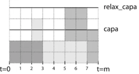
Over-loads are accepted in theSoftCumulativeSumconstraint and the objective variable (obj) represents the sum of the overloads. Figure 1 contains an example of this constraint.
relax_capa
t=0 1 2 3 4 5 6 7 t=m
capa
Fig. 1. Example ofSoftCumulativeSumwith a ground schedule with 3 fixed activities: a1
starts at 0 and ends at 3, and res[a1] = 2. a2starts at 2 and ends at 7, and res[a2] = 2. a3starts
at 5 and ends at 8, and res[a3] = 3. There is 3 over-loads: cost[2] = 1, cost[5] = 2, cost[6] = 2.
However, for some problems, constraining the sum of the over-loads is not enough. Some additional constraints w.r.t. these over-loads should be satisfied. A frequent requirement is to distribute fairly over-loads within a long time period, while limiting the number of big over-loads for each short period of time.
For instance, assume that the resource is the number of employees in a team. Each day (8 hours), each person contributes to some activities. An over-load will entail, in practice, either that extra-employees are hired, or that some activities are performed by a number of employees less than the number which was initially planed (for instance, some employees may accept to do homework). Typically, small over-loads (cost[t] = 1) correspond to the second case, while big ones (e.g., cost[t] > 3) require to hire extra-employees. Then, the number of each type of over-loads has to be limited, and these types are related one another. This means that the number of times a variable cost is greater than a given value has to be limited. Thus, we need to express that at most k variables can take a value v or greater.
This is the purpose of the new constraint OrderedDistribute. We define it
formally:
Definition 3.3. Let
• X be a set of variables
• T be an array of increasing values that can be assigned to variables in X, with |T | ≥ 2.
• Imax be an array of maximum possible number of occurrences of values in T , where Imax[i] corresponding to the value T [i], and such that ∀i ∈ {1, . . . , |T | − 1}, Imax[i − 1] ≥ Imax[i].
An assignment A(X) satisfies the constraint
OrderedDistribute(X, T , Imax) iff
(1) For each i ∈ {0, . . . , |T | − 1}, the number of values v in A(X) s.t. v ≥ T [i] is at most equal to Imax[i].
(2) The number of times value T [0] appears in A(X) is at least equals to |X| − Imax[1].
Observe thatOrderedDistribute also implicitly affects minimum occurrences of values: given an index i < |T | − 1, the number of times a value v ≤ T [i] appears in A(x) is at least equal to |X| − Imax[i + 1].
Example 3.1. We consider a human resource cumulative problem with 5 days of 8 hours, and a team of 8 employees. The following constraints are imposed w.r.t. over-loads.
(1) At most 5 over-loaded hours by day.
(2) At most 3 over-loads greater than or equal to 2.
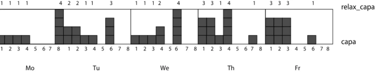
(3) At most 1 over-load equal to 4. (no over-load should exceed 4 employees). Here is a fully detailed instance. We consider 40 activities with the following dura-tions:[1, 1, 3, 1, 4, 2, 2, 1, 4, 4, 2, 4, 2, 3, 1, 2, 1, 1, 1, 2, 1, 3, 3, 2, 4, 3, 3, 1, 4, 2, 4, 2, 3, 4, 3, 4, 2, 3, 3, 2, 2, 2, 4, 4, 2, 4, 3, 4, 3, 4, 3, 2, 4, 4, 4]. Heights of activities are the following:[4, 2, 1, 1, 2, 3, 4, 1, 3, 3, 2, 1, 4, 4, 2, 3, 4, 1, 1, 1, 2, 4, 3, 3, 3, 1, 2, 4, 3, 2, 1, 4, 2, 3, 4, 1, 4, 4, 1, 2, 1, 1, 4, 3, 2, 2, 1, 3, 4, 4, 3, 2, 4, 1, 1]. capa Mo Tu We Th Fr 1 1 1 1 4 2 2 1 1 3 1 1 1 2 4 3 3 1 4 1 3 3 3 1 1 2 3 4 5 6 7 8 1 2 3 4 5 6 7 8 1 2 3 4 5 6 7 8 1 2 3 4 5 67 8 1 2 3 4 5 6 7 8 relax_capa
Fig. 2. Over-loads in the solution of Example 3.1.
Observe that an over-load of 4 is at least as undesirable as an over-load of 3, an over-load of 3 is at least as undesirable as an over-load of 2, and so on.
Figure 2 shows the over-loads in each day, in the cumulative profile corresponding to that instance. The sum of over-loads over the whole month is 48.
We can easily encode this problem by using theOrderedDistributeconstraint defined with T = [0, 1, 2, 3, 4] and Imax= [8, 5, 3, 3, 1] where T measures the over-loads and Imaxlimits the number of occurrences for each day. For instance, T [2] = 2 and Imax[2] = 3 means that we can have at most 3 times an over-load of size 2 or more for each day. The following model, written in pseudo-code, represents this problem.
// ds are the durations, hs the heights // capa and relax capa the capacities IntDomainVar[] start, costVar; IntDomainVar obj;
SoftCumulativeSum(start, costVar, obj, ds, hs, capa, relax capa); // additionnal constraints
T = [0, 1, 2, 3, 4]; Imax= [8, 5, 3, 3, 1];
for each day in a partition of costVar[]: OrderedDistribute(day, T, Imax)
// objective minimize(obj);
Here is a solution of the problem (each range [di, ei[ indicates the points in time where activity ai starts and ends in the schedule):
[30, 31[ [37, 38[ [32, 35[ [12, 13[ [0, 4[ [24, 26[ [21, 23[ [15, 16[ [0, 4[ [8, 12[ [35, 37[ [27, 31[ [26, 28[ [7, 10[ [38, 39[ [26, 28[ [31, 32[ [39, 40[ [39, 40[ [38, 40[ [39, 40[ [12, 15[ [23, 26[ [28, 30[ [8, 12[ [32, 35[ [32, 35[ [31, 32[ [10, 14[ [35, 37[ [32, 36[ [27, 29[ [32, 35[ [15, 19[ [13, 16[ [32, 36[ [29, 31[ [19, 22[ [32, 35[ [36, 38[ [38, 40[ [38, 40[ [0, 4[ [16, 20[ [36, 38[ [23, 27[ [37, 40[ [16, 20[ [20, 23[ [4, 8[ [23, 26[ [37, 39[ [4, 8[ [32, 36[ [32, 36[
More generally,OrderedDistributemay be useful in practice in several classes of problems:
• In bin-packing problems when objects have to be packed into containers. For instance, a fair distribution based on some degrees indicating frailty of the objects allows to limits the negative consequences (in terms of financial costs) of damaged containers.
• In assignment problems when teams have to be balanced with respect to the hierarchical skills of the members.
• In over-constrained problems, in which costs represent degrees of violation of constraints.b These costs are often strongly ordered. (Example 3.1 belongs to
this class.)
4. Reformulation of OrderedDistribute
Reformulating OrderedDistribute with existing cardinality constraints is not straightforward because limiting the maximum number of occurrences of a value v does not constrain the occurrences of all the values which are greater than v. It is necessary to augment such existing cardinality constraints with additional con-straints like arithmetic ones.
The most famous cardinality constraint is the global cardinality constraint or
Gcc. It is defined as follows:
Definition 4.1. Let X be a set of variables, T be an array of values, and I be the array of allowed integer ranges for each value of T .
An assignment A(X) satisfies the constraint Gcc(X, T , I) iff any value v = T [i]
appears in A(X) a number of times which belongs to I[i], i.e. #(T [i], A(X)) ∈ I[i], i = 0, . . . , |X| − 1.
Generalized Arc Consistency (GAC, see Section 2) can be established efficiently onGcc9,8.
When I are defined by boundaries of range variables (the card variables), the
Gccconstraint becomes thecardVar-Gccconstraint10. A range variable is a
vari-able which is represented by the minimum and the maximum values in its domain. Thus, the parameter I is replaced by the set of range variables Card, so as the signature iscardVar-Gcc(X, T , Card). Filtering algorithms forcardVar-Gcccan be found in10,8. Unfortunately, their time complexity is cubic.
Now, we can reformulate the OrderedDistribute constraint with a
cardVar-Gcc constraint and some arithmetic constraints.
Consider C =OrderedDistribute(X,T ,Imax). Let t = |T | − 1 and n = |X|. We define CN (C) the constraint network corresponding to theOrderedDistribute con-straint as follows:
• The variable set is X ∪ Card, where Card = {Card[0], ..., Card[t]} is a set of non negative integer variables.
• The constraint set if defined by the constraints: – ∀k = 0...t,Pt
i=kCard[i] ≤ Imax[k] – ∀k = 1...t,Pk−1
i=0 Card[i] ≥ n − Imax[k] – cardVar-Gcc(X, T , Card)
We explicitly add the second type of constraints because as far as we know solvers are not able to deduce from two sum constraints Pn
i=p+1yi ≤ a and P n
i=1yi = n that we havePp
i=1yi≥ n − a.
be concretely applied in practice, these problems can be view as optimization problems in which some constraints may be violated.
It is easy to check that this constraint network reformulates the constraint C (i.e., they have the same set of solutions). Unfortunately, this reformulation is weak even if the strongest filtering algorithms are used for each constraint, as shown by the following example:
Example 4.1.
Let X = [x1, x2, x3, x4, x5] be 5 variables such that D(x1) = D(x2) = {0, 1}, D(x3) = {0, 1, 2}, and D(x4) = D(x5) = {2, 3}. We consider the following con-straints :
(1) At most 3 xi greater than or equal to 1. (2) At most 2 xi greater than or equal to 2. (3) At most 2 xi equal to 3.
This example can be modeled by the constraint C =OrderedDistribute(X, T ,
Imax), with T = [0, 1, 2, 3] and Imax= [5, 3, 2, 2]. The constraint network associated with C involves the constraints:
(1) Card[3] ≤ Imax[3] = 2
(2) Card[2] + Card[3] ≤ Imax[2] = 2
(3) Card[1] + Card[2] + Card[3] ≤ Imax[1] = 3
(4) Card[0] + Card[1] + Card[2] + Card[3] ≤ Imax[0] = 5
(5) Card[0] + Card[1] + Card[2] ≥ |X| − Imax[3] = (5 − 2) = 3
(6) Card[0] + Card[1] ≥ |X| − Imax[2] = (5 − 2) = 3
(7) Card[0] ≥ |X| − Imax[1] = (5 − 3) = 2
(8) cardVar-Gcc(X, T , Card)
If the strongest filtering algorithms are used for CN (C) then the domains of the Card variables become D(Card[3]) = {0, 1, 2}; D(Card[2]) = {0, 1, 2}; D(Card[1]) = {0, 1, 2, 3}; D(Card[0]) = {2, 3}.
No value is removed from the domain of variables of X, whereas it should. Variables x4 and x5 can only take a value in {2, 3} and at the same time the number of times any value greater than or equal to 2 can be taken is 2, because of the constraint number 2) in Example 4.1. Therefore, no other variable can take a value in {2, 3} and so value 2 can be safely removed from D(x3).cardVar-Gccdoes
not remove such a value, because it considers, for instance, that x4 and x5 can take value 3 and then x3 value 2. In addition, note that the filtering algorithms associated with some constraints used in this reformulation are costly in practice. Thus, we have two reasons for designing an efficient filtering algorithm for the
5. Filtering Algorithms
5.1. Filtering Algorithm Based on Flow
First, we can note that it is possible to design a filtering algorithm based on flow as for the Gcc constraint. An algorithm in O(n2k) for checking consistency and establishing arc consistency is presented in6, where n = |X| and k = |T |. We will not detail the algorithm here, but we will give the main idea because it solves the issue with respect to the lack of filtering of the reformulation illustrated by Example 4.1. Moreover, it shows how some arithmetic constraints between cardinality variables can be integrated into a classical filtering algorithm forGcc. This technique might
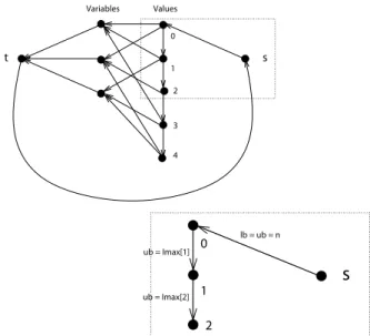
also be useful to deal with generalizations of theOrderedDistribute constraint. This filtering algorithm is based on the search for a flow of value n = |X| in a particular digraph. For convenience, we will denote by lb the lower bound capacity of an arc and by ub its upper bound capacity. Figure 3 is an example of such a digraph associated with anOrderedDistributeconstraint.
Definition 5.1. Let C =OrderedDistribute(X, T , Imax), we define the digraph G(C) = (XG, UG) as follows:
• XG= {s, t} ∪ X ∪ T . • UG contains:
– An arc (T [i], x) for each T [i] ∈ T and x ∈ X s.t. T [i] ∈ D(x). ub(T [i], x) = 1.
– An arc (T [i], T [i + 1]) for each i ∈ {0, . . . , |T | − 2} with ub(T [i], T [i + 1]) = Imax[i + 1].
– An arc (x, t) for each x ∈ X with ub(x, t) = 1. – An arc (s, T [0]) with ub(s, T [0]) = |X|.
– An arc (t, s) with lb(t, s) = |X| and ub(t, s) = |X|.
The main idea is to link the values together. In this way, the flow value which reaches a value v of T must pass by all the values less than v and so it is possible to count for these values the quantity of flow corresponding to the assignments of variables to values greater than them.
Proposition 5.1. Given C = OrderedDistribute(X, T , Imax) and its corre-sponding digraph G(C), the two following properties are equivalent:
• OrderedDistribute(X, T , Imax) has a solution. • There exists a feasible flow from t to s in G(C).
Once a feasible flow of value n has been computed in G(C), arc consistency can be established with the same algorithm as forGcc, so with a linear complexity.
Such a filtering technique requires to work with an additional data structure (the digraph associated with the constraint) and to compute and maintain a flow. In the next section we propose a simpler algorithm which is also more efficient in practice.
ub = Imax[2] Variables Values 2 3 4 t 1 0 s
s
0 1 2 ub = Imax[1] lb = ub = nFig. 3. Example of a digraph representing anOrderedDistribute(X, T , Imax). Arcs between
values and variables have a lower bound equal to 0 and an upper bound equal to 1. 5.2. Linear Filtering Algorithm
We first come up a consistency check forOrderedDistribute, in a time complexity
linear over the number of variables. Then, we come up with the linear GAC filtering algorithm.
By Definition 3.3, we have the following lemma.
Lemma 5.1. If OrderedDistribute(X, T , Imax) has a solution then Imax[0] ≥ |X|.
We define the assignment with all minimum values of domains.
Definition 5.2. The min-domain assignment of a set of variables X is the unique assignment A(X) of values to variables in X s.t. ∀x ∈ X, A(X, x) is equal to the minimum value in D(x).
Obviously, it is always possible to build a min-domain assignment if there is no empty domain, but this assignment does not necessarily satisfy the constraint. Proposition 5.2. Let A(X) be the min-domain assignment of an instance C of
OrderedDistribute. The two propositions are equivalent:
(α) #(T [0], A(X)) ≥ |X| − Imax[1]
and ∀i = 0, ..., |T | − 1: #(≥ T [i], A(X)) ≤ Imax[i]. (β) C has a solution.
Proof. (⇒) Suppose that (α) is satisfied. By definition 3.3, A(X) is a solution of C. (⇐) Suppose that C has a solution. By contradiction: assume that the min-domain
assignment A(X) of C does not satisfy (α). Two cases are (mutually) possible: (i) The number of times T [0] is assigned to a variable in A(X) is strictly less than |X| − Imax[1]. By Definition 5.2, any variable x s.t. T [0] ∈ D(x) is assigned to T [0] in A(X). Therefore, no other assignment can have a greater number of occurrences of T [0] and thus satisfies C, a contradiction. (ii) Assume that a value T [i] is s.t. #(≥ T [i], A(X)) > Imax[i]. By definition 5.2, if a value greater than T [0] is assigned to a variable x in A(X), this value is the minimum of D(x). Variables x in A(X) that take value T [i] cannot take a value strictly less than T [i]. No assignment exists with a lower value for #(≥ T [i], A(X)). C has no solution, a contradiction.
From Proposition 5.2 and Definition 5.2, the feasibility of an OrderedDis-tributecan be checked in O(n), where n = |X|.
Algorithm 1:isSatisfiable(OrderedDistribute(X, T , Imax)): boolean 1 if #(T [0], A(X)) < |X| − Imax[1] then
2 return false;
3 foreach T [i] ∈ T do
4 if #(≥ T [i], A(X)) > Imax[i] then return false;
5 return true;
Thanks to this procedure, time complexity of a flow-based algorithm (see Sec-tion 5.1) can be decreased to O(nk), where k = |T |. This time complexity can be improved again, by using an algorithm which does not require to work with an additionnal data structure.
We present now this dedicated filtering algorithm forOrderedDistribute. Next Corollary gives a sufficient condition for having all the values consistent withOrderedDistribute.
Corollary 5.1. Let C =OrderedDistribute(X, T , Imax), if ∀i ∈ {0, . . . , |T | − 1}, #(≥ T [i], A(X)) < Imax[i] then ∀x ∈ X, ∀v ∈ D(x), (x, v) is consistent with C. Proof. The assignment A0(X) obtained by replacing A(X, x) by v in A(X) is s.t. ∀T [i] ∈ T, #(≥ T [i], A0(X)) ≤ I
max[i]. By Definition 3.3, A0(X) is a solution of C.
Now, we can establish the corollary defining precisely the consistent values. Intuitively, there are two reasons for a value v ∈ D(x) not to be consistent. The first one is that its variable x must be assigned to T [0] to satisfy the minimum requirement and v > T [0]. The second one is that, a maximum of occurrences is reached for a value w ≤ v when all variables take their minimum value and x is assigned to a value u < w. Thus x cannot be assigned to v because in this case the number of value assigned to a value equal or greater than w are strictly greater
than Imax[k] with w = T [k]. We denote by X⊥ the set of variables whose domain contains T [0]: X⊥= {x ∈ X s.t. T [0] ∈ D(x)}.
Corollary 5.2. Let C be a feasibleOrderedDistribute(X, T , Imax) and A(X) be the min-domain assignment. A value v ∈ D(x) is not consistent with C if and only if one of the two following property is satisfied:
(α) x ∈ X⊥, v > T [0] and |X⊥| = |X| − Imax[1].
(β) ∃T [i] ∈ T, #(≥ T [i], A(X)) = Imax[i] and A(X, x) < Imax[i] and v ≥ T [i]. Proof. (α) is immediate. (β) By definition, if in A(X) a value is assigned to a variable x, this value is the minimum of D(x). Therefore, if T [i] satisfies #(≥ T [i], A(X)) = Imax[i], then given x ∈ X with A(X, x) < Imax[i], there exists no assignment A0(X) s.t. A0(X, x) ≥ Imax[i] and #(≥ T [i], A0(X)) ≤ Imax[i].
Algorithm 2:Filter(OrderedDistribute(X, T , Imax)) 1 if ¬ isSatisfiable(OrderedDistribute(X, T , Imax)) then
2 return;
3 A(X) ←min-domain assignment ofX ; 4 X⊥← {x ∈ X s.t.T [0] ∈ D(x)};
5 if |X⊥| = |X| − Imax[1] then
6 foreach x ∈ X⊥do
7 D(x) ← {T [0]};
8 T=← {T [i] ∈ T s.t.#(≥ T [i], A(X)) = Imax[i]};
9 X0← X;
10 while T=6= ∅ ∧ X0 6= ∅ do
11 Pick and remove the minimum valueT [i]in T= ;
12 foreach x ∈ X0 s.t. A(X, x) < Imax[i] do
13 Remove fromD(x)the set{v ∈ D(x), v ≥ T [i]} ; 14 X0← X0\ {x};
From Corollary 5.2 we obtain Algorithm 2. Values removed from a domain D(x) are necessarily strictly greater than A(X, x). It is necessary to evaluate each of these values (line 10) because some new variables can be reached when evaluating higher values in T= (defined in line 8), thanks to the condition of line 12.
This algorithm enforces GAC. Indeed, assume that a value T [i] ∈ D(x) is not consistent with the constraint after the run of the algorithm. This means that assigning T [i] to x entails in any complete assignment of X the existence of a value T [j] such that #(≥ T [j], A(X)) > Imax[j] and j ≤ i; especially in the min-domain assignment A(X). By construction of T= and from line 13 of the algorithm,
when T [j] ∈ T= was considered, T [i] was removed from D(x) by the algorithm, a contradiction.
Proposition 5.3. The time complexity of this algorithm is O(n+k), where n = |X| and k = |T |, provided that given v ∈ D(x), we can remove all values greater than v in O(1).
Proof. (Sketch) Values in T= (line 11) and in A(X) (line 12) can be sorted in increasing order in linear time by a counting sort since T is bounded. The total number of times lines 12 − 14 of the algorithm are executed is upper-bounded by |X|: if a variable is reached then it is removed from X0 by line 14. Thus the time complexity is in O(|T | + |X|)
Proposition 5.3 states that GAC can be enforced onOrderedDistribute with
a time complexity linear in the sum of the number of variables and the number of values in the union of their domains. Regarding the literature, we can note that some other simple generalizations ofGccare NP-Hard7.
We can adapt Algorithm 2 to make it incremental, by maintaining at least the following data:
• The min-domain assignment A(X).
• An array T#≥ counting, for each value T [i], the number of values w ≥ T [i] that appear in A(X).
However, even in this case, each time the counter of a value in T#≥ becomes such that T#≥[i] = Imax[i] it will be necessary to scan the variables in order to remove all the values greater than T#≥[i] for all variables having a value in A(X) strictly less than Imax[i]. Thus, time complexity remains in O(|X| + |T |), and it can be amortized on a given branch of the search tree only w.r.t. |T |, which is not very relevant : Algorithm 2 has a linear time complexity and there is generally a few number of cost values. The practical time cost for updating the stored data A(X) and T#≥ and the trail seems to be prohibitive. For the experiments we implemented Algorithm 2 with the version presented in this section.
6. Experiments
We experimented our global constraint on instances of the problem described in Example 3.1, which is derived from5, using the Java-based constraint programming engine Chococ.
We compared two representations ofOrderedDistribute.
• In the first one, we use the new global constraint we have defined. We name this model GlocalCt-Model.
• In the second one the constraint is replaced by a constraint network equivalent to the one proposed in Section 4. We name this model CN-model.
We tried for each model several search strategies. With the first model (GlobalCt-Model), the best results are obtained if, first, we first assign the minimum value to the start variable having the minimum-sized domain and then the same for cost variables. With the second model (CN-Model), the search strategy dom/wdeg2was the most efficient.
Instances involve n = 55 activities, m = 40 hours, durations between 1 and 4, resource consumption between 1 and 4, capa = 8, relax capa = 12. Costs at each point in time are from 0 to 4, the imposed distribution is for each day of 8 hours : At most 5 costs ≥ 1, at most 3 costs ≥ 2, at most 1 cost equal to 4.
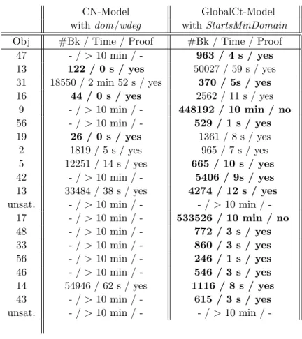
CN-Model GlobalCt-Model
with dom/wdeg with StartsMinDomain Obj #Bk / Time / Proof #Bk / Time / Proof
47 - / > 10 min / - 963 / 4 s / yes
13 122 / 0 s / yes 50027 / 59 s / yes
31 18550 / 2 min 52 s / yes 370 / 5s / yes
16 44 / 0 s / yes 2562 / 11 s / yes 9 - / > 10 min / - 448192 / 10 min / no 56 - / > 10 min / - 529 / 1 s / yes 19 26 / 0 s / yes 1361 / 8 s / yes 2 1819 / 5 s / yes 965 / 7 s / yes 5 12251 / 14 s / yes 665 / 10 s / yes 42 - / > 10 min / - 5406 / 9s / yes 13 33484 / 38 s / yes 4274 / 12 s / yes unsat. - / > 10 min / - / > 10 min /
-17 - / > 10 min / - 533526 / 10 min / no 48 - / > 10 min / - 772 / 3 s / yes 33 - / > 10 min / - 860 / 3 s / yes 56 - / > 10 min / - 246 / 1 s / yes 46 - / > 10 min / - 546 / 3 s / yes 14 54946 / 62 s / yes 1116 / 8 s / yes 43 - / > 10 min / - 615 / 3 s / yes
unsat. - / > 10 min / - / > 10 min /
-Table 1 gives the results obtained for instances such that no solution exists without over-loads (if there is no over-load thenOrderedDistributeis not useful).
Time limit is 10 minutes. The two unsolved problems have no solution satisfying the ordered cardinality constraints, but proving this unsatisfiability requires more
than 10 minutes.
These results show that the use of a generic heuristic dom/wdeg which is well-suited does not compensate the lack of filtering of the model CN-Model, except for a few number of instances which are easy to solve.
WithOrderedDistribute(GlobatCt-Model), 16 of the 20 instances are solved
and proved to be optimal in less than one minute (15 of them in less than 12 seconds), while the other model proves optimality only for 8 of the 20 instances. This latter model is not able to find a solution in a time less than 10 minutes for the 12 remaining instances. A few instances remain hard for the two models, since the optimum value cannot be found in less than 10 minutes. This is not surprising since searching for the minimum sum of over-loads in a soft cumulative problem (and proving optimality) is known to be a difficult problem.
7. OrderedDistribute with Range Variables
A natural extension of OrderedDistribute is to consider that maximum number
of occurrences of values are not scalar integers but a set of range variables. We distinguish two cases.
• The first one is obtained by replacing in Definition 3.3 the integer array Imax by an array of range variables R: the number of values greater than or equal to a given value v should be less than the value of its range variable in R. • The second one is similar to the first one except that the number of values
greater than or equal to a given value v should be equal to the value of its range variable in R.
7.1. OrderedDistributeRangeLeq
Definition 7.1. In aOrderedDistributeRangeLeq(X, T , R), we use the
param-eters described in Definition 3.3 except that R is a set of range variables. Given an assignment A(X), OrderedDistribute(X, T , R) is satisfied iff the two following
constraints are satisfied.
(1) #(T [0], A(X)) ≥ |X| − R[1].
(2) ∀i = 0, . . . , |T | − 1, #(≥ T [i], A(X)) ≤ R[i]
The consistency check remains the same than the one ofOrderedDistributeexcept that we replace Imax by the sequence of maximum values in domains of variables in R. The filtering algorithm remains the same concerning variables in X. It differs fromOrderedDistributew.r.t. lower bounds of domains variables in R: They may become not consistent withOrderedDistributeRangeLeqaccording to the current
domains of variables in X. For instance, for a value T [i] it may not remain enough values less than T [i] in domains of variables X to impose #(≥ T [i], A(X)) ≤ 0, so as 0 can be removed from R[i]. Minimum values for variables in R can be updated directly by counting, for each T [i], the number of variables in A(X) greater than or
equal to T [i]. This can be done incrementally while A(X) is built (note that A(X) remains the same after the filtering of variables in X). At last, increasing explicitly a lower-bound of a variable R[i] has no consequence except a fail if min(D(R[i])) > max(D(R[i])). Thus, GAC can be achieved on OrderedDistributeRangeLeq in O(n + k) time, with n = |X| and k = |T |.
7.2. OrderedDistributeRangeEq
In this section, we study the case where the number of values greater than or equal to a given value v should be equal to the value of its corresponding range variable. Definition 7.2. In aOrderedDistributeRangeEq(X, T , R), we use the
param-eters described in Definition 3.3 except that R is a set of range variables. Given an assignment A(X), OrderedDistribute(X, T , R) is satisfied iff the two following
constraints are satisfied.
(1) #(T [0], A(X)) ≥ |X| − R[1].
(2) ∀i = 0, . . . , |T | − 1, #(≥ T [i], A(X)) = R[i]
The filtering differs from OrderedDistributeRangeLeq. We need to compute the exact upper bounds of domains of variables in R (lower bounds are given by A(X) similarly toOrderedDistributeRangeLeq). Next example shows that such a computation does not simply consists in sorting the variables xi ∈ X by non decreasing max(D(xi)), then remove the first |X| − R[1] ones, and then count for each v ∈ T the number of values greater than v in domains of remaining xi’s. Example 7.1. Let X = {x1, . . . , x5} such that D(x1) = D(x2) = {0, 4}, D(x3) = {0, 3, 4}, D(x4) = D(x5) = {1, 2, 3}. T = [0, 1, 2, 3, 4]. Assume that D(R[4]) = [0, 1] and D(R[1]) = [0, |X|], and that we wish to prune D(R[3]), which is currently [0, 5]. The maximum possible value for R[3] is 4 because x1and x2cannot take both value 4.
Consider C =OrderedDistributeRangeEq(X, T , R). We search for each value v = T [i] the assignment satisfying C and having the maximum number of values greater than or equal to v. We show that it is enough to solve this problem in general. We propose to simplify the problem by only considering two values per domain of each variable.
Notation 1. Let v be a value in T . For any variable in X let min(x) be the minimum value of the domain and w(v, x) be the value of D(x) which is the nearest of v by excess (i.e. w(v, x) ≥ v and 6 ∃u ∈ D(x) with w(v, x) ≥ u ≥ v).
Property 1. Let v be a value in T and A(X) be any assignment satifying C with #(≥ v, A(X)) = j. Then, the assignment A0(X) defined from A(X) as follows:
• A0(X, x) = w(v, x) iff A(X, x) ≥ v
satisfies the constraint C and satisfies #(≥ v, A0(X)) = j.
Proof. Clearly we have #(≥ v, A0(X)) = j. In addition, since each value of A(X) is replaced by a smaller value it is clear that if A(X) satisfies C then A0(X) also.
We propose the following greedy algorithm:
(1) We order in L the variables by their non increasing min value. We break tie by non decreasing w value.
(2) We repeat the following process until L is empty:
We take the first variable x of L and remove it from L; and we assign w(v, x) to x if it does not violate C; otherwise we assign min(x) to x.
(3) The obtained assignment maximizes the number of values greater than v. To prove correctness of this algorithm we introduce two lemmas. Let A(X) be any assignment satisfying C and two variables x1and x2:
Lemma 7.1. Assume w(v, x1) = A(X, x1) and min(x2) = A(X, x2). If min(x1) ≤ min(x2) and w(v, x1) ≥ w(v, x2) then the assignment A0(X) with min(x1) = A0(X, x1) and w(v, x2) = A0(X, x2) and ∀y ∈ X − {x1, x2} : A0(X, y) = A(X, y) satisfies C and has the same number of values greater than or equal to v as A(X). Proof. A0(X) has obviously the same number of values greater than or equal to v as A(X). A(X) contains the set of value V and the values w(v, x1) and min(x2); and A0(X) contains the set of value V and the values min(x
1) and w(v, x2). Since min(x1) ≤ min(x2) and w(v, x2) ≤ w(v, x1) then if A(X) satisfies C then A0(X) also.
Lemma 7.2. Assume w(v, x1) = A(X, x1), min(x2) = A(X, x2), x1is the variable s.t. w(v, x1) < w(v, x2) and 6 ∃y ∈ X − {x1, x2} with w(v, x1) < w(v, y) ≤ w(v, x2) and #(≥ w(v, x2), A(X)) < R[k] and T [k] = w(v, x2). If min(x1) ≤ min(x2) then the assignment A0(X) with min(x1) = A0(X, x1) and w(v, x2) = A0(X, x2) and ∀y ∈ X − {x1, x2} : A0(X, y) = A(X, y) satisfies C and has the same number of values greater than or equal to v as A(X).
Proof. A0(X) has obviously the same number of values greater than or equal to v as A(X). A(X) contains the set of value V and the values w(v, x1) and min(x2); and A0(X) contains the set of value V and the values min(x1) and w(v, x2). We have w(v, x1) < w(v, x2) and #(≥ w(v, x2), A(X)) < R[k] and T [k] = w(v, x2) hence by exchanging w(v, x2) and w(v, x1) the assignment remains a solution.
We prove by induction that it is enough to assign w(v, x) to x when x has to be assigned and D(x) = {min(x), w(v, x)}. It is obviously true when there is only
one variable (if the min value is taken then the obtained assignment has less value greater than v than when w is taken).
Thus, consider that the current variable that has to be assigned within the greedy algorithm is x, with D(x) = {min(x), w(v, x)}. Suppose that we assign min(x) to x. We will show that we can obtain an equivalent or “better” solution (which maximizes the number of values greater than v) by taking w(v, x). After assigning min(x) to x, the greedy algorithm is continued and an assignment A(X) is computed. This assignment satisfies theOrderedDistribute constraint. Now, if
we impose A(X, x) = w(v, x) and if the assignment remains a solution then the current solution is improved and it is better to assign x with w(v, x). Therefore, we consider that this swap between min(x) and w(v, x) is not possible. Consider Y the set of variables assigned after x. Note that, by definition of the greedy algorithm any variable y ∈ Y satisfies min(y) ≤ min(x). Then, we have two possible cases:
• There exists a variable y ∈ Y with w(v, y) ≥ w(v, x). Then, Lemma 7.1 can be applied. This means that we can safely assign w(v, x) to x.
• Each variable y ∈ Y satisfies w(v, y) < w(v, x). We consider the one with the w value which is the closest to w(v, x) (that is, we define z ∈ Y satisfying 6 ∃y ∈ Y − {z} with w(v, z) < w(v, y) < w(v, x)). At the moment where x has been assigned, min(x) and w(v, x) were in its domain, therefore we had #(≥ w(v, x), Ap(X)) < R[k] and T [k] = w(v, x), where Ap(X) was a partial assignment. By the absence of variable of Y with w(v, y) = w(v, x) and by the definition of z it means that this property still holds for A(X). Therefore, Lemma 7.2 can be applied and we can safely assign x to w(v, x).
Thus, in all the cases it is safe to assign x to w(v, x) and this leads to an equivalent or better solution.
Property 2. The greedy algorithm can be applied for each value v of T with an overall time complexity in O(nk + k2).
Proof. (Sketch) The complexity for one value v depends on the computation of w(v, x) for each variable and the double sorts (check of consistency can be done in constant time each time a variable is fixed). Consider n = |X| and k = |T |. Each sort can be performed in O(k) by a counting sort. The computation of w(v, x) can be done for each variable in O(log(k)). So for one value v we obtain a complexity in O(n log(k) + k). However, when running the greedy algorithm for each value v we can amortize some computations: All the w values for a variable x can be computed in O(k) by traversing the domain while v is increased. Since there are k values to consider, the overall complexity is O(nk + k2).
8. Aggregations ofOrderedDistribute
The main usage ofOrderedDistributeis depicted by Example 3.1 and Figure 2: In order to obtain a particular distribution of costs, cost variables are partitioned and
an instance of OrderedDistributeis set on each subset of variables corresponding to a class of the partition. In the Example, a day is represented by a sequence of 8 cost variables representing over-loads during the 8 hours of this day. For each day an instance ofOrderedDistribute is set on the over-loads variables.
Additionally, an objective is usually defined over the whole set of cost variables, represented by an objective variable obj and an objective constraint. In the Example, we wish to minimize the sum of over-loads during a week of five days, that is, 40 cost variables.
We focus in this section on two classical cases for this objective constraint: either minimize the sum of costs, obj =P
x∈Xx, or minimize the maximum value assigned to a variable, that is, obj = maxx∈Xx.
Algorithm 3:AgFilterSum(OrderedDistribute OD[],obj, X) 1 LB ←Px∈X min(D(x));
2 U B ← max(D(obj)); 3 for j = 0 to |OD| − 1 do
4 ∆ ← U B − LB+Px∈OD[j].X min(D(x)); 5 if OD[j].Imax[1] > ∆ then
6 for i = 1 to |OD[j].Imax| − 1 do OD[j].Imax[i] ← min(OD[j].Imax[i], ∆);
/* Decrease too big OD[j].Imax[i] */; 7 k ← 1;
8 while k ≤ |OD[j].T | − 1 ∧ OD[j].T [k] ≤ ∆ do k ← k + 1; 9 for i = k to |OD[j].Imax| − 1 do OD[j].Imax[i] ← 0 ;
/* Set to 0 maximum occurrences of values in OD[j].T strictly greater than ∆ */; 10 Filter(OD[j]);
Consider a sequence X of variables, partitioned in subsequences such that an instance of OrderedDistribute is set on each subsequence. Let us first focus on
the case where the objective is a sum. The sum of minimum values in domains of variables in X provide a lower bound LB for the obj variable. From this lower bound, we can update arguments of each instance of OrderedDistribute before calling the filtering algorithm.
• If max(D(obj)) minus LB plus the sumP(min(D(xi)) of variables xi involved in the current instance of OrderedDistribute is greater than Imax[1], then we can safely decrease Imax[1]: The maximum number of values greater than or equal T [1] in a solution satisfying the objective constraint (more precisely, in a solution with an objective value less than or equal to max(D(obj))) is max(D(obj)) minus LB plus the sum P(min(D(xi)) of variables xi involved in the current instance of OrderedDistribute. The same reasoning can be applied on Imax[2], and so on, until the condition is not satisfied (recall that,
by Definition 3.3, values in the array Imax decrease as the index increases). • Since we make no hypothesis with respect to the implementation of the objective
constraint, quantity Imax[v] of values v which cannot be assigned to any variable in X without exceeding max(obj) can be set to 0.
Algorithm 3 implements these two principles.
The set of instances of OrderedDistribute are stored in an array OD[] of size |OD|, indexed from 0 to |OD| − 1. Arguments of one particular
OrderedDis-tributeat index j of the ODOrderedDistributearray are denoted respectively by
OD[j].X, OD[j].Imax, and OD[j].T . To simplify notations, Algorithm 3 considers that each OD[j].Imaxis storable: values which have been modified at this node are automatically re-assigned to the previous value when a backtrack occurs.
Algorithm 4 implements the same idea for the objective constraint obj = maxx∈Xx, using the same conventions. This case is simpler since one has just to avoid exceeding the maximum value of the objective variable obj.
Algorithm 4:AgFilteringMax(OrderedDistribute OD[],obj, X)
1 U B ← max(D(obj)); 2 for j = 0 to |OD| − 1 do 3 k ← 1;
4 while k ≤ |OD.T | − 1 ∧ OD.T [k] ≤ U B do k ← k + 1; 5 for i = k to |OD.Imax| − 1 do OD[j].Imax[i] ← 0;
/* Set to 0 maximum occurrences of values in OD[j].T strictly greater than U B */; 6 Filter(OD[j]);
Note that Algorithm 3 and Algorithm 4 can work with sets of variables and arrays Imaxwhich are different from an instance ofOrderedDistributeto another
one (not the same number of variables and not the same restrictions on occurrences).
9. Conclusion
In this paper we presented a new global constraint, OrderedDistribute, which
solves a practical modelling issue with respect to problems involving cost variables with strongly ordered domains. This constraint is complementary to global con-straints based on statistics, such asSpreadorDeviation. OrderedDistribute
ad-dresses those problems where variables can be carved in disjoint subsets, to control in a very precise way the number of occurrences of cost values within each subset. We provided a linear GAC filtering algorithm forOrderedDistribute. We experi-mented successfully our global constraint on a cumulative problem with over-loads.
References
1. A. Aggoun and N. Beldiceanu. Extending CHIP in order to solve complex scheduling and placement problems. Mathl. Comput. Modelling, 17(7):57–73, 1993.
2. F. Boussemart, F. Hemery, C. Lecoutre, and L. Sa¨ıs. Boosting systematic search by weighting constraints. Proc. ECAI, pages 146–150, 2004.
3. C. Mullinax and M. Lawley. Assigning patients to nurses in neonatal intensive care. Journal of the Operations Research Society, 53:25–35, 2002.
4. G. Pesant and J.-C. R´egin. Spread: A balancing constraint based on statistics. Proc. CP, pages 460–474, 2005.
5. T. Petit and E. Poder. Global propagation of side constraints for solving over-constrained problems. To appear in the Annals of 0perations Research, 2010.
6. T. Petit and J-C. R´egin. The ordered global cardinality constraint. Research report 09-07-INFO, ´Ecole des Mines de Nantes, 2009.
7. C.-G. Quimper. Enforcing domain consistency on the extended global cardinality con-straint is np-hard. Technical Report CS-2003-39, School of Computer Science, Uni-versity of Waterloo, 2003.
8. C.-G. Quimper, A. L´opez-Ortiz, P. van Beek, and A. Golynski. Improved algorithms for the global cardinality constraint. Proc. CP, 2004.
9. J-C. R´egin. Generalized arc consistency for global cardinality constraint. Proc. AAAI, pages 209–215, 1996.
10. J.-C. R´egin and C. Gomes. The cardinality matrix constraint. Proc. CP, pages 572– 587, 2004.
11. P. Schaus, Y. Deville, P. Dupont, and J-C. R´egin. The deviation constraint. Proc. CPAIOR, 4510:260–274, 2007.
12. P. Schaus, P. Van Hentenryck, and J-C. R´egin. Scalable load balancing in nurse to patient assignment problems. Proc. CPAIOR, 5547:248–262, 2009.