Chemical kinetic modeling of oxidation of hydrocarbon emissions in spark ignition engines

(1)

'CHEMICAL KINETIC MODELING OF OXIDATION OF

HYDROCARBON EMISSIONS IN SPARK IGNITION ENGINES

by Kuo-Chun Wu

Bachelor of Science in Mechanical Engineering National Taiwan University

(1990)

Submitted to the Department of Mechanical Engineering in partial fulfillment of the requirements

for the Degree of

MASTER OF SCIENCE IN MECHANICAL ENGINEERING at the

MASSACHUSETrs INSTITUTE OF TECHNOLOGY

February 1994

Signature of Author

Certified by

Department of Mechanical Engineering January 15, 1994

Simone Hochgreb Assistant Professor, Department of Mechanical Engineering Thesis Supervisor

Accepted by

Ain A. Sonin Graduate Committee

(2)

-CHEMICAL KINETIC MODELING OF OXIDATION OF HYDROCARBON

EMISSIONS IN SPARK IGNITION ENGINES

by Kuo-Chun Wu

Submitted to the Department of Mechanical Engineering on January 14, 1994 in partial fulfillment of the requirements for the Degree of

Master of Science in Mechanical Engineering

ABSTRACT

Hydrocarbon emissions from spark ignition engines are significantly affected by the type of fuel used. Furthermore, the type and amount of each chemical species leaving the exhaust are a very strong function of the fuel type. In order to model the process through which unburned hydrocarbons are oxidized in the exhaust process , one needs to take into account the transport of cold layers to the bulk gases and chemistry of oxidation of these mixtures. The objective of this work is to study the effect of fuels on the resulting hydrocarbon emissions by using existing detailed chemical kinetic mechanisms of oxidation of hydrocarbons. Because of computational time constraints, only fully-mixed time-dependent problems were considered. A parametric study of the effects of pressure, equivalence ratio, temperature and fraction of unburned gas on characteristic chemical time scales for fuel oxidation and total hydrocarbon oxidation were made to provide useful information about hydrocarbon oxidation under relevant kinetically-controlled conditions. In addition, detailed kinetic models have been used to investigate the interactions between two components in a binary fuel, which is the first step for exploring the influence between different types of components in real fuels. Moreover, one-step expressions have been fitted from the numerical results of detailed chemical mechanisms so they can be used in more sophisticated transport models for better predictions. Correlations between reaction time and total hydrocarbon emissions from engines operating on single substance fuels show the practical use

of the simple zero dimensional approach.

A second part of the work was devoted to combine a simple physical thermal model and detailed chemical kinetic models to simulate the oxidation of unburned hydrocarbons through the exhaust port. The results show that measured extents of oxidation of the unburned fuel through the exhaust cannot be reproduced by the simulations using the well mixed (average) temperatures in the exhaust, but that the experimental results can be bracketed by the average and core temperatures. Investigations of the temperature limits for kinetic control in the exhaust port, the effect of super-equilibrium radicals, and the behavior of intermediate combustion products were made for further understanding the mechanisms of hydrocarbon oxidation. The analysis shows that most of the oxidation occurs at the very early exhaust times, when temperatures in the exhaust are in excess of approximately 1200 K. For the fuels considered, it is suggested that oxidation is controlled by mixing rates at the initial stages of exhaust, where temperatures are high and the cold unburned mixture emerges from the wall layers in to the exhaust jet.

Thesis Advisor: Simone Hochgreb,

(3)

ACKNOWLEDGMENTS

I am very grateful to have Professor Simone Hochgreb as my research advisor. I am deeply thankful for her encouragement, guidance, patience, and kindness. I would also like to acknowledge Professors John B. Heywood and Wai K. Cheng for their thoughtful suggestions and valuable insights. In addition, I would like to thank Mike Norris for performing the engine and exhaust simulations; Todd Tamura and Koji Oyama for their assistance in testing the chemical kinetic mechanisms; Kristine Drobot for carrying out the exhaust quenching experiments; and members of the Industrial Consortium on Engine-Fuels interactions and CRC Consortium, for their invaluable comments and funding support.

I cannot say enough about all the friends that I have met here, who have warmed my heart and supplied me with the energy to complete this work. In, particular, I am most fortunate to have Kuo-Chiang as my partner, for we went through the best and worst times and bad times together. I am also grateful to Ann and Arthur Yang, Cynthia Chuang, Sean Li, Jasmine Lin, Phillips Nee, Shane Shih, Chuang-Chia Lin, Tung-Ching Tseng, George Wang, and Shirley Hsu for their timely care, support and friendship. They have made the sometimes lonely and arduous study at MIT much easier and memorable. I have also enjoyed the friendship and scientific assistance of Mike, Dr. Lee, Koji, Gatis, Wolf, Kristine, Kyoungdoug, Pat, Joan, Karla, and all the other students of my laboratory.

Finally, very special thanks are extended to my family: my parents, Mr. Shaw-Chii Wu and Mrs. Yu-Chuan Wang, and my sister and brother, Kuo-Ying and Kuo-An. Their endless support and encouragement made me realize that, no matter how things would turn out, they would always be there for me. This thesis is dedicated to them.

Cambridge, MA January 1994

(4)

LIST OF TABLES

2.1 Chemical kinetic mechanisms used in simulations 6

3.1 Ranges of parameters used in simulations 18

3.2 Coefficients of one-step expressions for fuel destruction 33 3.3 Coefficients of one-step expressions for overall hydrocarbon conversion 34 3.4 Coefficients of one-step expressions for overall hydrocarbon conversion 35

(7)

LIST OF FIGURES

Figure 2.1: Figure 2.2: Figure 2.3: Figure 3.1: Figure 3.2: Figure 3.3: Figure 3.4: Figure 3.5: Figure 3.6: Figure 3.7: Figure 3.8:

A schematic view of the hydrocarbon emissions mechanisms. Simulated in-cylinder temperature and pressure for the baseline case of Kaiser et al.[5] (top) (>=-0.9, 1500 rpm, 3.75 kpa IMEP, MBT spark timing. Fuel: propane), and simulated deviation of in-cylinder hydroxyl (OH) mole fractions from the equilibrium state

as a function of crank angle (bottom).

Mole fractions of propane and its primary products of partial oxidation for T=1200 K, unburned mixture fraction: 1%, >-=0.9.

(top) burned gas composition in equilibrium at 1200 K; (bottom) burned gas composition from the in-cylinder simulation at 1200 K.

Mole fractions of propane and its primary products of partial oxidation for T=1000 K, Xu (unburned gas fraction)=0.01, at

(top) lean mixture (=0.9); (bottom) rich mixture (=-1.15). Mole fractions of n-butane and its primary products of partial oxidation for T=1000 K, Xu (unburned gas fraction)=0.01, at (top) lean mixture ((I)=0.9); (bottom) rich mixture (=-1.15). Mole fractions of iso-octane and its primary products of partial oxidation for T=1000 K, Xu (unburned gas fraction)=0.01, at

(top) lean mixture (0=0.9); (bottom) rich mixture (=1.15). Mole fractions of toluene and its primary products of partial oxidation for T=1000 K, Xu (unburned gas fraction)=0.01, at

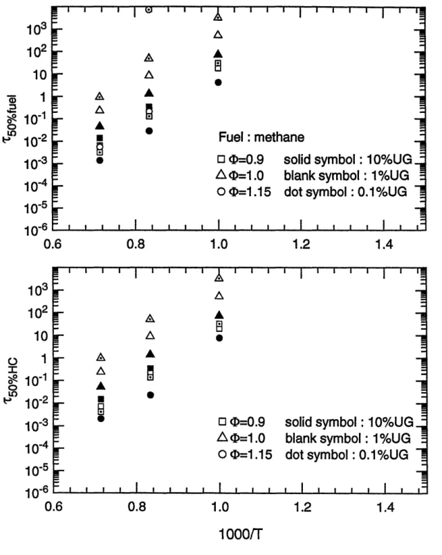
(top) lean mixture (-0.9); (bottom) rich mixture (45=1.15). Characteristic 50% reaction time scales for methane as a function of the reciprocal temperature for (top) fuel destruction; (bottom) overall hydrocarbon conversion.

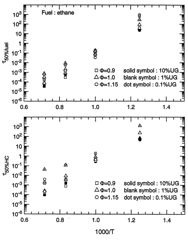
Characteristic 50% reaction time scales for ethane as a function of reciprocal temperature for (top) fuel destruction; (bottom) overall hydrocarbon conversion.

Characteristic 50% reaction time scales for propane as a function of reciprocal temperature for (top) fuel destruction; (bottom) overall hydrocarbon conversion.

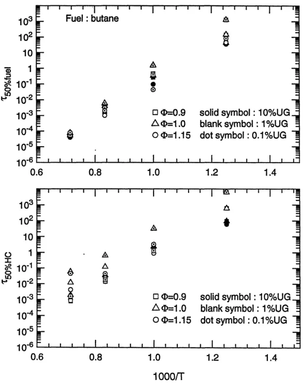
Characteristic 50% reaction time scales for n-butane as a function of reciprocal temperature for (top) fuel destruction; (bottom) overall hydrocarbon conversion.

14 15 16 36 37 38 39

40

41 42 43

(8)

Figure 3.9: Figure 3.10: Figure 3.11: Figure 3.12: Figure 3.13: Figure 3.14: Figure 3.15: Figure 3.16: Figure 3.17: Figure 3.18: Figure 3.19: Figure 3.20:

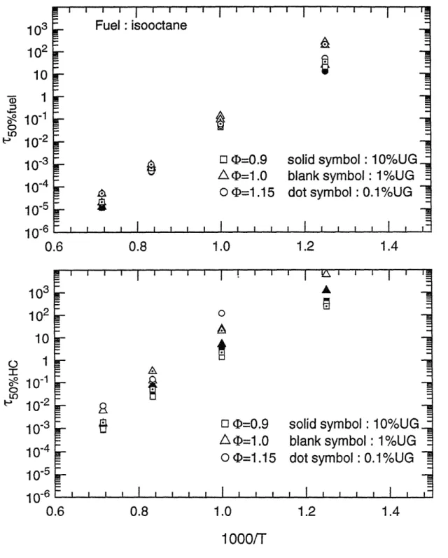
Characteristic 50% reaction time scales for iso-octane as a function of reciprocal temperature for (top) fuel destruction; (bottom) overall hydrocarbon conversion.

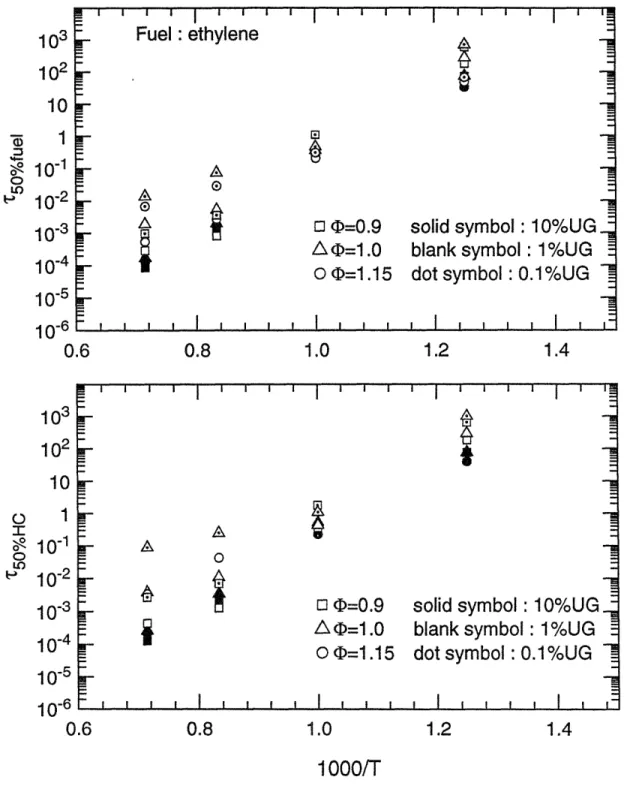
Characteristic 50% reaction time scales for ethylene as a function of reciprocal temperature for (top) fuel destruction;

(bottom) overall hydrocarbon conversion.

Characteristic 50% reaction time scales for propene as a function of reciprocal temperature for (top) fuel destruction;

Characteristic 50% reaction time scales for 1-butene as a function of reciprocal temperature for (top) fuel destruction; (bottom) overall hydrocarbon conversion.

Characteristic 50% reaction time scales for toluene as a function of reciprocal temperature for (top) fuel destruction; (bottom) overall hydrocarbon conversion.

Characteristic 50% reaction time scales for methanol as a function of reciprocal temperature for (top) fuel destruction; (bottom) overall hydrocarbon conversion.

Characteristic 50% reaction time scales for MTBE as a function of reciprocal temperature for (top) fuel destruction;

Calculated ratio of the 50% reaction times at 1 atm to 10 atm as a function temperature for several selected fuels. (>=-1.0, 10% unburned mixture)

A comparison of the extents of fuel destruction for (top) paraffins; (bottom) olefins, oxygenated fuels, and toluene in an burned gas environment: P=1 atm, (D=1.0, T=1200 K, and 1% unburned gas mixture.

A comparison of the extents of overall hydrocarbon conversion for (top) paraffins; (bottom) olefins, oxygenated fuels, and toluene in an burned gas environment: P=l atm, D=1.0, T=1200 K, and 1% unburned gas mixture.

A comparison of practical residence times in SI engines (lines) and calculated half lives of fuels (symbols) during oxidation in a burned gas environment as a function of reciprocal temperature: P=l atm, 4-=1.0, and initial concentration: 1% unburned gas mixture.

A comparison of practical residence times in SI engines (lines)

44 45 46 47 48 49 50 51 52 53 54 55

(9)

and calculated half lives of total hydrocarbon (symbols) during oxidation in a burned gas environment as a function of reciprocal temperature: P=l atm, i=-l.0, and initial concentration: 1% unburned gas mixture.

Figure 3.21: Figure 3.22: Figure 3.23 Figure 3.24: Figure 3.25: Figure 3.26: Figure 3.27: Figure 3.28:

The ratios of characteristic reaction times for (top) fuel destruction (bottom) hydrocarbon conversion computed from one-step expressions to full kinetic mechanisms as a

function of timt. (Fuel : propane)

A comparison of the predictions of the behaviors of fuel

destruction and overall hydrocarbon conversion from a one-step mechanisms (dashes lines) and a detailed chemical kinetic mechanism (solid lines). Fuel : propane. A good match in the predictions of characteristic reaction times from two models is

achieved in this case.

Calculated ratio of half lives for fuel oxidation and total hydrocarbon oxidation (=0.9, P=1 atm, Xu=10%), plotted as a function of measured fraction of unburned fuel in the total hydrocarbons

Calculated half lives for fuel oxidation plotted as a function of measured normalized hydrocarbon emissions (4=0.9, P=l atm, Xu=10%). Two calculated values are shown for methane, for a plug flow and a stirred reactor simulation.

Calculated profiles of mole fractions of propane and ethylene in a burned gas environment as a function of time: P=l atm, T=1200 K,

total initial concentration: 1000 ppmC1. The ratio of initial concentration (propane : ethylene = 4: 1). The calculated profiles of pure fuel destruction with the corresponding initial concentrations are also plotted for comparison.

The effects of intermediate byproducts on the calculated extent of fuel reaction for ethane, propane, butane, and isooctane. (T= 1200 K, unburned mixture fraction: 1%, ~(=0.9)

Calculated extent of fuel destruction for unburned mixture with different intermediates addition (ethane, ethylene, or formaldehyde) for methane. (T=1200 K, unburned mixture fraction: 1%, =0.9) Comparisons of calculated extents of fuel destruction for (top) butane and (bottom) toluene for different proportions of initial concentrations between two fuels in the 1% unburned mixtures. The corresponding extent of reaction of pure fuel in the 0.1% unburned gas are also plotted for comparison.

56 57 58 59 60 61 62 63

(10)

A schematic view of the cross section of an engine exhaust port Figure 4.2: Figure 4.3: Figure 4.4: Figure 4.5: Figure 4.6: Figure 4.7: Figure 4.8: Figure 4.9: Figure 4.10:

Calculated average temperatures for each mass element leaving the cylinder at two different speeds (top) and corresponding fuel concentration profiles for each element as a function of crank angle (bottom). Fuel: propane, initial concentration: 300 ppmC1. Operating conditions: I=0.9, 3.75 kpa IMEP.

Calculated extent of reaction in the exhaust port (lines) and measured values (symbols, blank symbol : 2500 rpm, dot symbol: 1500 rpm) for two different operating conditions. Operating conditions : >0.9, 3.75 kpa IMEP.

Calculated core and average temperatures in cylinder and exhaust port as a function of crank angle. The drop in temperature for each element leaving the cylinder is due to heat loss to the walls. Operating conditions: 4=0.9, 1500 rpm, 3.75 kpa IMEP.

Calculated extent of reaction in the exhaust port (lines) and measured values (symbols). Solid lines are simulations performed with core temperatures (no heat loss to the exhaust walls),

dashed lines are simulations with average temperatures. Operating conditions: cb=0.9, 3.75 kpa IMEP.

A comparison of calculated extent of reaction in the exhaust port using plug flow model and stirred reactor model. Both simulations

are performed with the assumption of no heat loss to the walls. The symbol represents the experimental measurement value. Operating condition: cb=0.9, 1500 rpm, 3.75 kpa IMEP, MBT spark timing.

Calculated extent of (top) fuel destruction and (bottom)

hydrocarbon conversion for n-butane as a function of temperature at the different residence times. (P=1 atm, <4 0.9, Xu=1%) Calculated extent of (top) fuel destruction and (bottom) hydrocarbon conversion as a function of temperature at the residence time of lms. (P=l atm, )=0.9, Xu=1%).

Calculated limits for mixing-controlled and kinetically controlled oxidation regions in the port for a residence time of 1 ms.

Controlling limits shown for propane oxidation.

Comparisons of calculated extent of fuel and hydrocarbon reaction as a function of time in an equilibrium burned gas environment and in a non-equilibrium burned gas environment at 1400 K(top left),

1200 K(top right), 1000 K(bottom left), and 800 K(bottom right). Fuel: butane, (P=l atm, (D=0.9, Xu=10%)

77 78 79 80 81 82 83 84 85 Figure 4.1: 76

(11)

Figure 4.11: Figure 4.12: Figure 4.13: Figure 4.14: Figure 4.15: Figure A.1: Figure A.2: Figure A.3:

Comparisons of calculated extent of fuel and hydrocarbon reaction as a function of time in an equilibrium burned gas environment and in a non-equilibrium burned gas environment at 1400 K(top left),

1200 K(top right), 1000 K(bottom left), and 800 K(bottom right). Fuel: butane, (P=1 atm, (I=0.9, Xu=1%)

Comparisons of calculated extent of fuel and hydrocarbon reaction as a function of time in an equilibrium burned gas environment and in a non-equilibrium burned gas environment at 1400 K(top left), 1200 K(top right), 1000 K(bottom left), and 800 K(bottom right). Fuel: butane, (P=l atm, <D=0.9, Xu=O.1%)

Comparisons of extent of reaction in the exhaust port for isooctane with different initial concentration profiles. Operating conditions: (I=0.9, 1500 rpm ,3.75 kpa IMEP.(all of profiles have only one

4500 ppmCl high step just as shown in the top plot except for profile F, which has one peak at beginning as profile A and the other peak at the end as profile D)

A comparison of calculated extent of reaction in the exhaust port for pure methane and the mixture of 95% methane plus 5% ethane. Solid lines are simulations performed with core temperatures (no heat loss to the exhaust walls), dashed lines are simulations with average temperatures. Operating condition :)=0.9, 1500 rpm, 3.75 kpa IMEP, MBT spark timing.

Calculated extent of fuel reaction as function of temperature at the residence time 1 ms for propane and ethylene. (top left) and the reaction profiles for the uniform mixture of propane and ethylene

(propane: ethylene = 4: 1) at (A) 1400 K(top right) (B) 1200 K (bottom left), and(C) 1000 K (bottom right). (P=l atm, =0.9)

A comparison of experimental results [19](square symbol) and computed results (circle-line) of ignition delay times for mixture of isooctane, oxygen, and argon. All mixtures contain stoichiometric amount of isooctane and oxygen at approximate 2 atm pressure, with 70% argon diluent.

Comparisons of experimental results [22](symbols) and computed results (lines) of ignition delay times for mixture of toluene, oxygen, and argon. All mixtures contain stoichiometric amount of toluene and oxygen at 2 atm pressure, with 95% argon diluent. (square symbols, circle-line), 6 atm pressure, with 95% argon diluent. (circle symbols, triangle-line), and 2 atm pressure, with 85% argon diluent. (triangle symbols, square-line), respectively. Comparisons of experimental results [24](symbols) and computed

86 87 88 89 90 143 144 145

(12)

results (lines) of ignition delay times for mixture MTBE, oxygen and argon. All mixtures contain stoichiometric amount of MTBE and oxygen at 3.5 bar pressure, with initial compositions of MTBE/02/Ar in the ratios 0.3/2.25/97.45 (cross symbols and circle-line), 0.6/4.5/94.9 (square symbols and triangle-line), and 1.2/9.0/89.8 (diamond symbols and square-line), respectively.

(13)

CHAPTER 1

INTRODUCTION

1.1 Background

Hydrocarbon (HC) emissions from spark ignition (SI) engines have faced increasingly stringent regulations since the United States Clean Air Act of 1970 and, with the adoption of the United States Clean Air Act of 1990, further tightening of hydrocarbon emissions is under way. Therefore, tailpipe emissions are a critical consideration for engine system designers, who must optimize for emissions, fuel economy, performance, cost, and durability. In addition, new fuels, such as alcohol fuels, are also being tested as alternatives to mitigate the effects of hydrocarbon products emitted into the atmosphere. With this in mind, automotive companies in collaboration with research institutions, and universities have recently engaged in extensive experimental and analytical studies in order to clarify the mechanisms of production and reduction of hydrocarbon emissions from spark ignition engines for control of hydrocarbon emissions.

1.2 Relevant experiments and analytical approach

Perhaps because of the relative complexity of processes involved the development of fundamental physical and chemical models of hydrocarbon formation and oxidation in the cylinder and exhaust system are still in their infancy. A few physically based, semi-empirical models have been developed for the formation of hydrocarbons via crevices, quench and oil layers, and partial bum, followed by in-cylinder or port oxidation [1-3]. Other investigators used more sophisticated fluid mechanical models [4,5] to correlate observed trends with engine operating conditions. These models have also utilized empirically fitted parameters for the

(14)

calculation of oxidation of rates of hydrocarbons, and did not attempt to quantify the products of partial oxidation.

The extensive tests performed under the Air Quality Improvement Research Program have generated a large and useful database on the effect of different fuel variables on total and speciated emissions from spark ignition engines [6]. Other researchers have experimentally studied the effect of single-species fuels on emissions at steady state operation [7-10]. In particular, recent hydrocarbon emissions experiments were performed on simple, pure fuels by Kaiser et al. [7-9]: lean and rich mixtures were studied at steady engine operating conditions, and the effect of changing engine speed and spark timing was investigated for the lean mixtures. This work is particularly useful for comparison with the present numerical results because the different fuels were studied in the same engine under the same operating conditions, and because chemical kinetic mechanisms have already been formulated for these small hydrocarbons.

1.3 Motivation and objectives

Although the current federal regulation specifies maximum values for the total non-methane organic gas (NMOG), the speciated hydrocarbon emissions are of increasing importance because the state of California will regulate hydrocarbon emissions based on their reactivity in forming ozone in the atmosphere in the near future [12]. In addition, even though experiments indicated that fuel effects on hydrocarbon emissions are relevant [7-9], there has been no attempt to incorporate them into modeling. Therefore, the purpose of the current work is the application of fully detailed chemical kinetic mechanisms to investigate evolution of oxidation processes of unburned fuel, combustion intermediates, and total hydrocarbons in the ranges expected to be encountered in the cylinder and exhaust port using zero-dimensional models without transport. The objectives are to:

(15)

· determine how the parameters (temperature, equivalence ratio, unburned mixture fraction, and pressure) influence the characteristic times of hydrocarbon oxidation. * correlate the zero-dimensional simulation results with experimental data

* fit one-step expressions for fuel destruction and hydrocarbon oxidation to produce approximate estimations of reaction rates over the relevant conditions

* investigate the interactions between the different types of fuels and how the intermediate combustion products affect the behavior of their parent fuels

* incorporate the physical engine simulation models with full chemical mechanisms to study the exhaust port oxidation process

· quantitatively and qualitatively analyze the experimental and simulated results of the oxidation of hydrocarbons in the exhaust.

(16)

CHAPTER 2

APPROACH and MODEL

2.1 Background

During the normal combustion process in spark ignition engines, a fraction of the fuel inducted into the cylinder is prevented from burning through storage in cold wall layers, generally called hydrocarbon sources [11] (crevices, deposits, oil layers, and flame quenching, shown in Fig. 2.1) . These unburned hydrocarbons emerge out of the different sources into the burned gas during the expansion and exhaust process and some of the unburned hydrocarbons exit the cylinder into the exhaust port and manifold. Oxidation occurs in the cylinder and exhaust system as hydrocarbons mix with the bulk burned gas. The oxidation of the unburned hydrocarbons is governed both by the rate of mixing into the burned gas as well as by the chemical kinetic rate of oxidation. However, transport processes cannot currently be combined with the detailed chemistry mechanisms because the computational expense of such of a treatment would be prohibitive. Therefore, efforts to incorporate some of these processes into two dimensional fluid mechanical models (KIVA) have only used one-step reduced chemical reaction mechanisms [4,5]. No attempts have been made at modeling the hydrocarbon oxidation during the expansion and exhaust processes in spark ignition engines using a detailed chemical kinetics model. In addition, critical experimental information about the nature of turbulence near the liner walls, as well as on the thickness of thermal boundary layer around the regions where unburned hydrocarbons emerge is scarce. Hence it is very difficult to predict the unburned hydrocarbon oxidation processes with accurate transport models coupled with full chemistry. Nevertheless, because of the possible regulation on speciated hydrocarbon emissions based on their reactivity in forming ozone in the atmosphere in the near future [12], and experimental indication that fuel

(17)

effects on hydrocarbon emissions are relevant, the focus of the current work is to apply existing chemical kinetic mechanisms of oxidation of hydrocarbons to the engine hydrocarbon emissions problem using zero-dimensional, time-dependent modeling. Real fuels are clearly too complex to be realistically modeled at present. Only single component fuels such as simple paraffins, olefins, oxygenated fuels, and aromatics whose detailed chemical mechanisms of oxidation are currently available are studied. For zero-dimensional modeling, more attention was given to port oxidation instead of in-cylinder oxidation, since zero-dimensional model is more suitable for modeling the former. More details on modeling and approaching the hydrocarbon emissions problem are described as following.

2.2 Chemical kinetic mechanisms

Because reduced chemical mechanisms determined from experimental data or detailed chemical kinetics calculations have been typically validated only for specific conditions (particularly flame propagation) or for very narrow parameter ranges, they are not suitable for the present purposes. In addition, simplified mechanisms usually do not provide information on the intermediate species formed during the reactions. "Comprehensive" detailed chemical kinetic mechanisms which have been validated over a wide range of conditions (pressure, temperature, and equivalence ratio) make possible the prediction of chemical behavior under a wide range of conditions. In general, interpolation within the range of conditions covered by a comprehensive mechanism is more reliable than extrapolation from a model validated at a single set of conditions. Therefore, detailed chemical kinetic mechanisms were used to simulate hydrocarbon oxidation.

All the detailed, elementary step mechanisms for the current study were drawn from the literature. Present detailed chemical schemes for oxidation simulation have included four straight-chain paraffins (methane, ethane, propane, n-butane), one branched-chain paraffin

(18)

(isooctane), one aromatic fuel (toluene), and two oxygenated fuels (methanol and MTBE). In the interest of consistency, chemical kinetic mechanisms for the oxidation of methane, ethane, propane, and n-butane validated over wide temperature, pressure, and equivalence ratio with jet-stirred reactor and shock tube data were chosen from the same group (the work of Dagaut, Cathonnet and coworkers [13-16]). The mechanisms for methane and ethane include the same reactions and rate parameters since the methyl radical recombination chemistry is included in the methane mechanism [13]. The propane mechanism was a subset of that of butane, since chemical reaction models are often constructed in a hierarchical manner. Furthermore, models for simple olefins (ethylene, propene, and 1-butene) were already included in kinetic models for their parent paraffins (ethane, propane, and n-butane) since olefins are byproducts of paraffin oxidation. Detailed reaction mechanisms for large molecules: isooctane, toluene, and MTBE were included because of the interest in their behavior within real fuels, even though they have been only validated with limited experimental data. The mechanism for MTBE is a combination of reaction mechanisms of MTBE, isobutene, [21] and n-butane [16]. Table 2.1 lists the sources for the chemical kinetic mechanisms used and the parameter ranges over which they have been validated.

All the chemical kinetic mechanisms for the oxidation study were verified against published experimental data using the CHEMKIN interpreter and integration computer codes [26]. In particular, more experimental data ([18],[19],[22],[25]) than those available in the original literature have been compared with the mechanisms which had been only validated at narrow range of conditions in order to check the possibility of extension of these models (see Appendix). However, since validation is still limited by the lack of experimental data available, the results of the simulations have to be considered with caution. As an example, in the MTBE mechanism, some modifications were made to pre-exponential factors of reactions C4H9OCH3 + X = C4H9OCH2 + HX (increased by a factor of 10 , where X refer to H, 0, OH, and H02 radicals) and C4H9OCH3 = IC4H8 + CH30H (increased by a factor of 2) to match flow reactor data [25] and shock tube data [24].

(19)

Table 2.1. Chemical kinetic mechanisms used in simulations

Fuel Reference Apparatus* T (K) P (atm)

methane [13] JSR 900 - 2000 1 - 13 0.1 - 2.0 ethane [14] JSR 800- 2000 1 - 10 0.1 - 2.0 propane [15] JSR 900 - 2000 1- 10 0.15 - 4.0 n-butane [16] JSR 900 - 2000 1- 10 0.15 - 4.0 i-octane [171/[18] PFR 1080/1135-1235 1.0 0.99/0.5-2.2 [19] ST 1250-1450 1.74.8 0.99 toluene [20,21] PFR 1188,1190 1.0 0.69,1.33 [22] ST 1334-1611 2.0-6.0 0.33-1.0 methanol [23] PFR 1025-1090 1.0 0.6-1.6 MTBE [24] ST 1100-1600 3.45 1.0 [251 PFR 1024,1115 1.0 0.95

* Experimental data used in mechanism validation. JSR: jet stirred reactor, PFR: plug flow reactor, ST: shock tube

2.3 Physical models

An accurate simulation for the hydrocarbon oxidation process would include chemical reactions and species transport effects. However, this is computationally infeasible at this point in time. This section describes the physical models used in the current computations which do not include transport phenomena. The plug flow reactor model was used for calculating the characteristic time scales and port oxidation simulations. Results using the perfectly stirred reactor (PSR) model were also studied and compared to those of the plug flow reactor model. Both are described below. Finally, the engine-exhaust simulation models which generated histories of the mass flow rate exiting the cylinder and the cylinder and exhaust port gas temperature and pressure to drive the detailed chemical port oxidation simulations are described.

(20)

Plug flow reactor model

An important class of idealized combustion systems are collectively called plug flow reactors. These systems are characterized by high linear flow rates with negligible recirculation flow. Each element of gas reacts as it moves, with the characteristic time scale for heat and mass transfer by diffusion in the cross stream direction being much faster than that for convective motion so that each cross section has uniform properties. Therefore, for a reacting system without turbulent or molecular transport, the species and temperature evolution equation is:

Dyi

w.

DT

_

wihio

i= Wi and

DT

=

_

wihi

Dt

p

Dt

pCp

where yi is the mass species concentration, wi the mass reaction rate and p the local mass density. The operator

D

a

dx a

-- + .

Dt at dtax

For steady one dimensional flow,

a = 0

and

x

dx

Dyi

a

dyi

O and

=

so

that

=v

=

a

t

at

dt

Dt

ax

dt

For purposes of comparison to experimental data in steady flow, distance is converted to time by means of velocity measurements. Based on the assumption of this model, gas flow which contains the burned and unburned mixture is discretized into several sections, and there are no temperature, pressure, and concentration gradients existing in each element of mixture.

Stirred reactor model

Another important idealized combustion system which can be considered to be spatially uniform is the perfectly stirred reactor (PSR). The PSR utilizes rapid mixing to achieve spatial homogeneity. Reactants are injected at a uniform rate into a combustor through a number of inlets. Within the perfectly stirred reactor, reactions take place, and energy is released in the uniform region, and the product gases (with the same properties as the uniform region) are

(21)

removed through the exhaust opening. The characteristic time scale is the average residence time in the reactor. Thus, a well-stirred reactor can be modeled as a flow system in which a mixture flows into a control volume where it is perfectly mixed with recirculation flow of combustion products, which flow out at the same conditions as those prevailing inside the chamber, so that the governing equation for a steady perfectly stirred reactor is:

Yi - Yio wi (y,,T)

I P

where, y (O) = Yio and y () = yi.

A comparison of calculation results of plug and stirred reactor models

From a physical point of view, the plug flow model is an isolated, moving control volume (if we interchange the space coordinates with time, we can treat it as a static control volume) which contains the homogeneous reacting mixture; and the perfectly stirred reactor model is a control volume where steady-state incoming and outgoing flows cross over and uniform mixing of new inflows and remaining mixture occurs continuously at an infinite rate. From a numerical point of view, modeling plug flow reactor requires solving systems of time-dependent initial value problems; modeling well-stirred reactors requires solving systems of boundary value problems. The kinetic equations for plug or stirred reaction models were integrated using the CHEMKIN library which will be described in the following section. Plug or stirred reactor calculation results for the extent of reaction as a function of residence time differ only very little for the same inlet conditions and isothermal reaction, with exception of methane, for which time scales are one order of magnitude shorter for the perfectly stirred reactor model. Therefore, in the following chapters, the plug flow reactor model will be used for characteristic time scale computations and exhaust port oxidation simulations, and the results of well-stirred reactor models will be compared with those of plug flow models where they are obviously different.

(22)

Engine simulation models

For the simulations of hydrocarbon oxidation in the exhaust port, which will be discussed in Chapter 4, data about the temperature and initial concentration history through the exhaust port must be obtained in order to drive the detailed chemical kinetic models. However, there are not enough data available on the accurate time-resolved temperature profile for exhaust gases through the exhaust port so far. Therefore, engine and exhaust port thermal simulation models must be used to predict in-cylinder and port temperature histories and the mass flow rates exiting the cylinder in order to drive the simulation of hydrocarbon oxidation in the port.

A two-zone, zero-dimensional thermodynamic model for the state of the gas in a four-stroke spark ignition engine [271 was used to predict the pressure and temperature of the gas and the mass flow rate through the valves as a function of crank angle. The total mass exiting the cylinder was discretized into ten elements and the temperature histories in the exhaust port were calculated for each mass element based on heat transfer relationships derived by Caton et al. [28] based on experimental measurements of exhaust temperatures. A plug flow model was used for each exhaust gas element, and the initial conditions for the exhaust temperature were calculated from the thermodynamic model of the engine cylinder mentioned above; the boundary conditions for the in-cylinder and port calculations were obtained from the bulk thermal model of the entire engine [29], which predicts the engine component temperature, including the coolant and oil circuits and the exhaust system.

2.4 Numerical methodology

The solution to the systems of ordinary differential equations of the detailed chemical kinetic schemes were made using the CHEMKIN-II chemical kinetics package [26]. This set of

(23)

CHEMKIN is a fortran software package for the solution of gas-phase chemical kinetic problems. The chemical kinetic reactions and a thermodynamic database which contains appropriate thermochemical information (specific heat at constant pressure, standard-state enthalpy, and entropy) of species involved in the reactions are read by its interpreter, and a binary linking file which holds all the pertinent information on elements, species, and reactions in the mechanism is produced for use by CHEMKIN subroutines and other application codes. The thermodynamic data for most of the species involved in the simulation were obtained from Kee et al. [30], and Burcat et al. [31]. The computer program THERM [32], which uses the group additivity method, was used to calculate the thermochemical coefficients of the species not available in the CHEMKIN database. Nevertheless, since the data computed from THERM have uncertainties associated with the inputs, reverse reaction rate constants have been included in the current chemical reaction mechanisms if available in the literature, rather than from forward rate constants and equilibrium constants calculated using the thermodynamic database.

For the simulations of plug flow reactors and shock tubes, CHEMKIN-based application code named SENKIN (Lutz et al., 1991) was used which predicts homogeneous gas-phase mixture chemical kinetics by integrating the time dependent conservation equations of species and energy. The characteristic time scales in the plug flow model which will be discussed in detailed in Chapter 3 are calculated at constant pressure and temperature; simulations of shock tube models are computed based on the assumptions of constant density (volume) and adiabatic condition. This code has been also modified in order to include the option of varying temperature and pressure histories. This temperature and pressure programming is used to determine the levels of super-equilibrium radicals in the exhaust gas using the predicted in-cylinder temperatures and pressures. In addition, the exhaust port hydrocarbon oxidation simulations were carried out by temperature programming at constant pressure in SENKIN. In addition to SENKIN, the PSR program [33] was used to compute the simulations of perfectly stirred reactors; and the initial composition of gas mixture at equilibrium is obtained by running the

(24)

2.5 Approach

In order to determine chemical reaction time scales of unburned hydrocarbons in burned gas mixtures, homogeneous mixtures of the bulk burned gas and various concentrations of unburned mixture assumed to consist of unreacted air and fuel (unburned mixture fraction) were considered as the initial composition for the present zero-dimensional computations. The composition of the burned gas consists of products of combustion of the gaseous fuel under equilibrium conditions, or non-equilibrium as described below. Since active radicals (OH, H, O), which are responsible for the attack on the unburned hydrocarbons, do not recombine at a rate sufficiently high to match the equilibrium composition during the expansion process in the cylinder, the effect of non-equilibrium radical concentrations was initially investigated. The predicted in-cylinder pressures and temperatures (Fig. 2.2), from the engine simulations were used for kinetic temperature and pressure programming in order to simulate how the non-equilibrium radicals deviate from the non-equilibrium states. Initial conditions for these simulations are the assumptions that the burned gases are mixture in chemical equilibrium at peak pressure. Figure 2.2 also depicts the deviation of hydroxyl (OH) concentration from the equilibrium state as a function of crank angles (CAD). The radical concentrations depart from equilibrium by one order of magnitude at exhaust valve opening (EVO). The effect of super-equilibrium radicals on the evolution of hydrocarbon oxidation is illustrated in Fig. 2.3(a) and (b). Figure 2.3(a) shows a typical plot of concentrations of fuel and partial oxidation products, starting with a mixture of burned gas in equilibrium and unburned fuel-air mixture at 1200 K. Figure 2.3(b) shows the effect of using initial conditions at 1200 K with super-equilibrium radicals from the engine simulation: there is immediate reaction with excess radicals, followed by a behavior similar to that of Fig. 2.3(a) for a mixture of equilibrium burned products. Note that the time scale for the overall reaction is not significantly affected by the different radical concentrations, and that the profiles of stable intermediates are almost identical as a function of extent of reaction of fuel. Accordingly, for simplicity purposes of comparison among fuels, the chemical characteristic time

(25)

scales involved in the oxidation of fuels and total hydrocarbons are investigated as a function of temperature, pressure, equivalence ratio, and fraction of unburned mixture in an equilibrium burned gas mixture using a zero-dimensional, detailed chemistry calculation. The exhaust port oxidation process was assumed to be that of a perfect mixture of unburned gas and burned gas which contains the super-equilibrium radicals traveling through the exhaust port subject to programmed temperature history. Details about the initial conditions for defining the characteristic time scales and calculating the extent of port oxidation will be described in the following chapter.

(26)

~a

ŽC) IC) !-U ._ _ 3 W

la

L-CC

C)O

0 -

₀

L

:)za

j O -C* C) C _a;..

U

'O

a

A schematic view of the hydrocarbon emissions mechanisms.

C) U C C) .- 0 C .O

.)C

Cc

L}_

C

'

a0 D

CY E

_'5

O-E(

M %&-t, C U S; >

a

Figure 2.1: I

(27)

]u'

103 E

Q. -

10

-1

t1

r-2

I

400

500

600

700

----zU

15 E

10

U3 0) a,

5 n

Z5UU

2000

7 1500

0 E

F-1000

400

500

600

700 Crank angle

Figure 2.2: Simulated in-cylinder temperature and pressure for the baseline case of Kaiser et al. (top) [5] (=0.9, 1500 rpm, 3.75 kpa IMEP, MBT spark timing. Fuel: propane), and

simulated deviation of in-cylinder hydroxyl (OH) mole fractions from the equilibrium state as a function of crank angle (bottom).

_- I I ' I I I " ' ' I I I 'I

in-cylinder simulation

...

Equilibrium

EVO

I...,

_

I

~~~~~.

.. -A r .

(28)

1500

0

Q. 1000

500

A 10-5 10-4 10-3 10'2 10-1

1500

1000

500 n

1

o5

10-4

10

10-2 10-1

Time (sec)

Figure 2.3: Mole fractions of propane and its primary products of partial oxidation for T=1200 K, unburned mixture fraction: 1%, )=0.9.(top) burned gas composition in equilibrium

(29)

CHAPTER 3

PARAMETRIC STUDY OF HYDROCARBON OXIDATION

3.1 Introduction

Because of limitations on computer time, and by insufficient available experimental information for detailed physical models of the oxidation process of hydrocarbon emissions in spark ignition engines, the problem of hydrocarbon emission modeling was initially approached by application of detailed chemical kinetic to perform zero-dimensional computations for a uniform mixture of burned gas at different initial temperatures, pressures, and compositions expected to be encountered in the process of hydrocarbon oxidation through the cylinder and exhaust. Using these chemical models (mostly comprehensive mechanisms validated over a range of conditions) a group of systematic numerical predictions have been made. These results provide systematic information about the possible chemical behavior of unburned hydrocarbons over a wide range of conditions. Not only did the simulation results supply a clearer picture about the role of hydrocarbon oxidation in spark ignition engines in a quantitative sense, but they were also used to fit reduced one-step mechanisms to produce approximate estimations of reaction rates over the relevant conditions that can be used in more sophisticated models including fluid mechanics and heat transfer effects.

Parameter matrix

Since hydrocarbon oxidation occurring in the cylinder and exhaust port is an unsteady and non-uniform phenomenon, the current study used four parameters (pressure, temperature, equivalence ratio, and fraction of unburned gas in the mixture), which vary with time and space

(30)

during the exhaust process, so that the parameter matrix would bracket the situations in the engines. The ranges of parameters are listed in Table 3.1 and will be discussed as follows.

Table 3.1 Ranges of parameters used in simulations

Parameter Range

Temperature (K) 800, 1000, 1200, 1400 Fuel/Air equivalence ratio ·( 0.9, 1.0, 1.15

Unburned mixture fraction (%) 0.1, 1.0, 10

Pressure (atm) 1.0, 10

(a) Temperature

As will be shown in Section 3.3, the simulation results show that when the temperature is above 1400 K, most hydrocarbons are burned within 0.1 millisecond, roughly 1 crank angle for an average 1500 rpm engine speed; when the temperature is below 800 K, the mixture composition is practically frozen. Therefore, the range 800-1400 K is focus of our present interest, even though the temperature range spans a wider range than this during the expansion and exhaust processes.

(b) Fuel/air equivalence ratio ()

The definition of equivalence ratio is that the ratio of the actual fuel/air concentration ratio to the stoichiometric ratio.

([Fuel] )actual

=

[Air]

( 3.1)

([Fuel] )stoich

(31)

Equivalence ratios 0.9, 1.0 and 1.15 have been used for the parametric study to check the evolution of species involved in the oxidation processes under lean, stoichiometric and rich conditions, respectively. Typical operating conditions are stoichiometric, with small excursions to the lean and rich sides. These specific values were originally selected for comparison with existing experimental results [5].

(c) Unburned mixture fraction

The unburned mixture fraction is the ratio of the volume of unburned gas mixture to the volume of total mixture which includes the burned and unburned gas. Based on the ideal gas law, this gas volume ratio equals the molar ratio. From the assumption of perfect and adiabatic mixing, the fraction of unburned cold gas is limited if the final mixture temperature is to be higher than a minimum temperature of 800 K. Therefore, 10%, 1%, and 0.1% of unburned gas in the whole mixture were selected. Typical fuel molar fractions in the exhaust are of the order of 2000 ppmCl, which roughly equals 1 to 3% unburned mixture fraction.

(d) Pressure

Pressure values between 1 and 10 atm were chosen for the current parametric study because these values correspond to the range of pressures among which unburned hydrocarbons start outgassing from sources and emerge at temperature low enough for the chemical time scales to be controlling (Fig. 2.2).

Computation details

There are 72 ( 2 ( 1, 10 ATM) * 4 ( 800 K, 1000 K, 1200 K, and 1400 K) * 3 ( equivalence ratio 0.9, 1.0, 1.15 ) * 3 ( 10%, 1%, and 0.1% unburned gas fraction ) ) simulations for each fuel. For each simulation, the initial composition of mixture is a combination of the composition of equilibrium burned gas, which is calculated using STANJAN [34] and that of unburned gas which includes fuel and the corresponding amount of air. The ratio of fuel to air is

(32)

according to the assigned equivalence ratio and composition of the air is assumed to be only oxygen and nitrogen ( 02 _: N2 = 1 : 3.773 ). For the current study, it is assumed that the

unburned mixture is coming from the crevice or wall quenching, and that the mixture consists of a fixed ratio of air and unburned fuel. Hydrocarbons emitted from the oil layers and deposits typically consist of fuel only and have not been studied in detail, since the very rich case is beyond the validated range of present models. Computation starts at the specific initial composition of the mixture, constant pressure and temperature.

3.2 Speciation results

One of the advantages of detailed chemical kinetic mechanisms is the ability to follow the evolution of all chemical species. The total hydrocarbon concentration (in ppmCl) obtained by adding up the mole fraction of all species times the number of carbon in each molecule (C1) except for carbon monoxide (CO) and carbon dioxide (CO2), is then an index of the extent of the

oxidation of the original fuel.

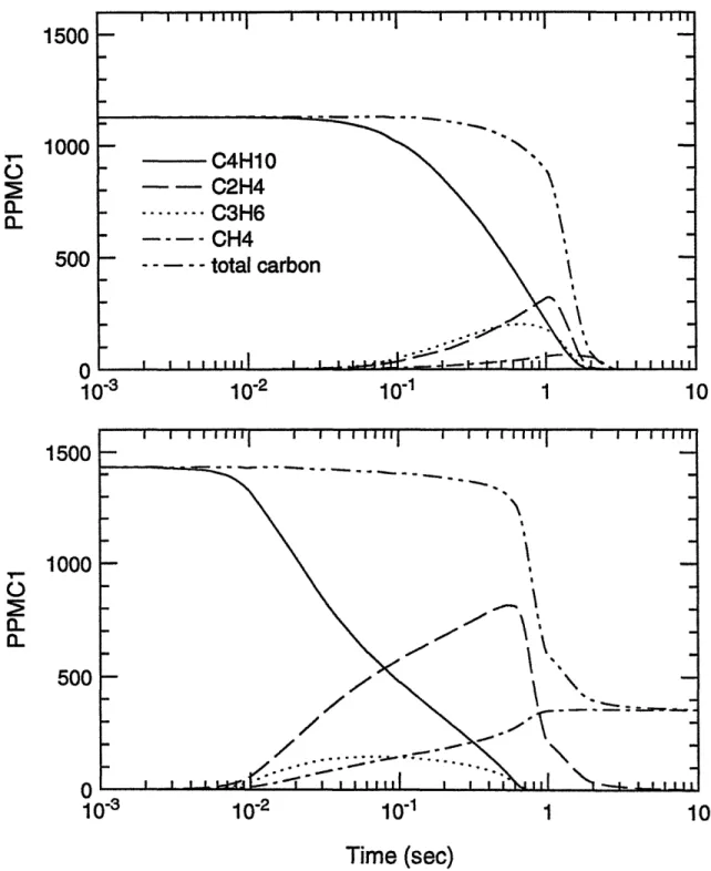
Figures 3.1 to 3.4 show the evolution of major species for propane, n-butane, iso-octane, toluene under fuel lean ( = 0.9) and rich ( = 1.15) conditions. Since the previous simulation results [35] indicated that the distributions of products is not significantly changed by temperature or initial concentration, but strongly affected by the equivalence ratio, the simulations for 1% unburned gas at 1200 K can provide enough information about the hydrocarbon oxidation process.

The simulated results showed that the type and proportion of major products is primarily a function of the structure of the compound and equivalence ratio. For example, ethylene and propene are the major products of propane and n-butane oxidation, both straight-paraffinic fuels. Iso-octane, which is a branched-paraffinic fuel, produces a large amount of iso-butene; and a large of amount of methane is produced at rich conditions rather than lean conditions. In

(33)

addition, results showed that the time scales for fuel decomposition and total carbon conversion are of the same order of magnitude for smaller molecular fuels such as methane, ethane, ethylene, propane, n-butane and methanol. However, carbon conversion times are much longer than the fuel decomposition times for larger molecular fuels such as iso-octane and MTBE. These observed trends can be explained by the fact that large molecules break easily into many small, longer-lived segments so that it takes much more time to oxidize all the species into carbon monoxide and carbon dioxide.

3.3 Time scale results

Time scales for oxidation of fuels under plug-flow conditions provide useful quantitative benchmarks for further understanding of the oxidation rate of hydrocarbons. The time scales for the oxidation of a fuel or total carbon is defined here as the time at which 50% of the fuel was reacted and 50% of carbon was converted into CO or CO2, respectively. Computations showed

that 50% reaction times are of the same order of magnitude as 10% or 90% reaction time for most simulation cases. Therefore, the half lives of hydrocarbons represent time scales at which the complete conversion of hydrocarbons occurs.

Parametric effects

The effect of five parameters (temperature, fuel/air equivalence ratio, fraction of unburned gas, fuel type and pressure) was investigated. Although in general it is easy to predict the qualitative trends of oxidation rates according to the trends of temperature and pressure, quantitative measures of sensitivity require detailed analysis. In addition, changes in one parameter can cause change in more than one rate-determining factor so that it is hard to decide the trend of oxidation speed directly by qualitative predictions. For instance, reducing the fraction of unburned gas in the mixture makes the concentration of fuel smaller so as to retard the

(34)

reaction rate; on the other hand, the effect of the extra oxygen in the burned gas may speed up reactions at fuel lean conditions when the unburned gas concentration becomes smaller. Therefore, only systematic numerical simulation results provide a clear picture about how these parameters quantitatively affect the reaction time scales.

(a) Temperature effect

The 50% reaction time scales of the whole fuel matrix as functions of the reciprocal of temperature are shown in figure 3.5 (a) to 3.15 (a), for fuel decomposition; and in figure 3.5 (b) to 3.15 (b), for carbon conversion, respectively. These plots obviously show that temperature is the most important parameter on the oxidation time scales. Within the temperature range of interest, 800 K to 1400 K, the time scales span six orders of magnitude. In particular, reaction times change by two orders of magnitude with a 200 K change in temperature.

Data points whose times exceed 104 seconds (3 hours) are not shown in the graphs. This occurs because of the low temperature for some unreactive species or lack of oxygen in the carbon conversion process. Considering the practical residence time scales in spark ignition engines, reactions can be treated as frozen if the time scale is beyond 1 second. This point will be discussed later.

(b) Fuel/air equivalence ratio effect

Compared to temperature, equivalence ratio has little effect upon time scales for oxidation. Except for methane and toluene, calculation results at fuel/air equivalence ratio 0.9 ( lean), 1.0 ( stoichiometric ), and 1.15 ( rich ) conditions showed that the variations of the half-lives of fuels are within one order of magnitude. Moreover, for most cases the changes in reaction times were within a factor of three. Computations indicated that reaction times for methane are more sensitive to equivalence ratio, changing by an order of magnitude difference in 50% reaction times was made by the relatively narrow variations of equivalence ratio. This may probably be explained by the fact that the stable molecular structure of methane makes the

(35)

decomposition of methane more difficult than other fuels so that the conversion times are more dependent on the concentration of fuel and oxygen.

One thing should be noticed is that because the lack of oxygen at fuel rich conditions (D = 1.15) the 90% of conversion of total carbon into carbon monoxide (CO) and carbon dioxide (C02) is hard to achieve, even the 50% conversion may be achieved and probably the time scales

be the same order of magnitude as those at lean and stoichiometric conditions.

(c) Unburned mixture fraction effect

Similarly to the effect of equivalence ratio, the concentration of unburned gas does not affect the conversion times very much. For most simulation results, the variations are limited within the same order of magnitude. For the most stoichiometric and rich conditions, the reaction times are longer when the unburned mixture fractions become smaller. Conversely, there are opposite trends observed at most fuel lean conditions. Although not all simulated results are consistent with the tendency described above, the exceptions are still within a factor of two, which may be accounted within the range of uncertainties ( model accuracy, or the precise representative meaning of 50% reaction time ( only one points) for the whole oxidation process etc.). The explanations for these observations are apparently that the dilution of burned gas slows down the reaction rates since the concentrations of fuel and oxygen become small, but the extra oxygen, whose concentration is large relative to that of the unburned fuel, in the burned gas speeds up the reactions at the fuel lean conditions. The most apparent trends are observed for the simulated results of methane.

(D) Pressure effect

At the same temperature, higher pressure means that the density and the collision rates are higher. Therefore, in general time scales are shorter if the pressure increases. Simulation results showed that the time scales are moderately affected by varying the pressure from 1 atm to 10 atm. The ratios of two time scales (1 atm : 10 atm) vary from nearly one to roughly an order

(36)

of magnitude and the values strongly depend on temperature and fuel type (shown in Fig 3.16). The effect of pressure on the time scales and the dependency of the fuel type is smaller at high temperature than at low temperature. Since chemical kinetic models for iso-octane and toluene were not validated at high pressure in their original publications and the shock tube experimental data were usually carried out at higher temperatures, the simulated results should be used with caution.

(e) Fuel type effect

The extent of reaction as a function of time for the entire fuel matrix is plotted in Figs. 3.17 (a) and (b), for the parent fuels, and in Figs. 3.18 (a) and (b), for the total hydrocarbon under the conditions of 1200 K, 1 atm, stoichiometric fuel/air ratio, and 1% unburned fuel-air mixture. The rank of oxidation rates changes little with temperature (Figs. 3.5 - 3.15), since the different groups of fuels have similar activation energies. Methane shows the slowest oxidation rate of the hydrocarbons tested, followed by toluene, both fuels of well-known stable chemical structure. The fastest rates of fuel decomposition were found for ethane, isooctane, MTBE and methanol; the fastest oxidation speeds for total carbon were found for ethane, ethylene, and methanol. Since the rate of decomposition of intermediate products is in general different from that of the fuel itself as discussed above, fuel destruction times are shorter than overall carbon conversion times. The difference is very apparent for the large molecules such as iso-octane and MTBE, since they rapidly decompose into longer-lived intermediate hydrocarbons. Therefore, in the current test matrix, isooctane and MTBE have fast fuel decomposition times but their carbon conversion times are not the fastest. The fastest carbon conversion rates were found for smaller molecules such as ethane, ethylene, and methanol which produce less intermediate products.

A comparison with residence time scales in spark ignition engines

The range of temperatures where oxidation rates are likely to control hydrocarbon destruction in spark ignition engines can be obtained by an order-of-magnitude comparison

(37)

between the chemical kinetic time scales and the residence times of internal combustion engines. A group of fuels was selected to make this comparison: methane, n-butane, isooctane (two paraffins which are significant components of real fuel), toluene (important component of real fuels), MTBE, methanol (oxygenated fuels) and -butene (olefinic fuel). Because of the differences observed between results from plug flow model and stirred reactor model for methane, both results were plotted for comparison. Furthermnnore, since temperature is the primary parameter controlling time scales, comparisons were made for constant pressure (1 atm), fuel/air ratio ( = 1.0), and fraction of unburned gas (1% of unburned fuel-air mixture) and various temperatures (800 K, 1000 K, 1200 K, and 1400 K). Figures 3.19 and 3.20 show the calculated half lives for fuel and total carbon oxidation for selected fuels as a function of reciprocal temperature. Typical residence times for the exhaust gas are also indicated in the same figure. Ten milliseconds is the order of magnitude of the in-cylinder residence time process, 1 to 100 milliseconds is the range of the residence time for the exhaust gas through the exhaust port, if both of the conditions of gas passing through and staying in the port after EVC (exhaust valve closed) are considered. Therefore, the time scale comparison shows that above approximately 1400 K all hydrocarbons are completely oxidized in less than the residence time of 10 milliseconds, conversely, there is no substantial oxidation below 1000 K at the longest residence times of 100 milliseconds.

3.4 Global expressions

In order to explore more realistic fluid mechanical models, simplified one-step expressions are desirable to minimize computational time, at the expense of chemical detail and accuracy. There exist already many reduced mechanisms in the literature for the simpler hydrocarbons. However, most have been developed for flame propagation, which is in general very different from the problem considered here. In the former, temperatures are high (> 2000 K),

(38)

molecular diffusion dominates and many reactions are partially equilibrated, none of which are necessarily true in the low temperature, turbulence mixing situation considered in hydrocarbon emissions problems. One-step expressions representing the approximate trends of the oxidation of hydrocarbons were obtained from the detailed models for further exploration of the emission problems. The procedure for fitting one-step expressions from the data sets calculated from the detailed chemical kinetic mechanisms and comparisons with simulations of full kinetic models will be discussed below.

Approach

According to the definition of characteristic reaction rate, the current global expressions are defined as a pseudo first order rate:

E

Ld[f]

1 dIIHC]

- = A(pfo )a(p )e

(

_RT

_(3.2)

[f] dt

[HC] dt

X

Pfo : Initial fuel concentration ( mole/cm

3

)

po

: Initialoxygenconcentration(

mole/cm

3

)

R

: Universal gas constant( 1.986 kcal/kmolK )

T

: Temperature ( K )

The characteristic reaction rate of the fuel or overall hydrocarbon is defined as the time derivative of the natural logarithm of fuel concentration. It obviously corresponds to the reciprocal characteristic reaction time t, at which l/e of original fuel or total carbon still remains unreacted.

variables are the initial fuel and oxygen concentration, temperature. The pre-exponential term A, and the dependence on fuel (a), oxygen concentration (fi), and the activation energy E are unknowns obtained by fitting the numerical simulation results.

In general, there are 36 data points used for fitting the global mechanisms, : 4 (temperatures : 800 K, 1000 K, 1200 K, and 1400 K) * 3 (equivalence ratios ·D: 0.9, 1.0, and

(39)

1.15) * 3 (unburned mixture fraction: 10%, 1%, and 0.1%) * 1 (pressure: 1 atm), corresponding to the characteristic time for ( 1-l/e ) reaction at each condition. Some data points were excluded from the set as they exceed the assigned maximum time limit (104 seconds), so that there are less than 36 points used for fitting the one-step expressions in some cases. The global mechanisms

are fitted by standard square error minimization.

Results

The fitted parameters a, [5, and E for the one-step expressions for the whole test matrix are listed in Table 3.2 and Table 3.3, for fuel decomposition and for carbon conversion, respectively. For the predictions of characteristic reaction times for fuel destruction, Methane results are poorly predicted at rich conditions; and toluene has those poor results for rich conditions at 800 K. The poorest results have one to two orders of magnitude differences in the predicted characteristic times. Fitted expression for ethane and ethylene are the poorest predictions of total hydrocarbon conversion times for the conditions that the equivalence ratio equals 1.15 and unburned mixture fractions are 1% and 0.1%. Except for these few poor results, most of these expressions can make reasonable approximations, which almost all the estimating times are within the same order of magnitude as full mechanism data. A comparison for propane is shown in Fig 3.21. Under low temperature rich conditions the carbon conversion into CO or CO2 is very difficult to be completed and the first order decay behavior of hydrocarbons

specified from the one-step models cannot reproduce this behavior. Accordingly, a set of coefficients for the hydrocarbon oxidation was calculated by only including lean and stoichiometric cases. Table 3.4 lists the expressions which only apply to lean and stoichiometric conditions. An improvement of the accuracy of prediction of characteristic time scales of hydrocarbon conversion for all fuels was observed by entirely excluding the rich cases from the data sets. Better predictions for fuel destruction times from methane and toluene one-step expressions can also be achieved by excluding the exceptional cases. (For methane, all rich cases are excluded; for toluene, only the conditions of 800 K and ( = 1.15 are excluded from the