Controlled formation of nanostructures with desired geometries : robust dynamic paths to robust desired structures

Controlled formation of nanostructures with

desired geometries: Robust dynamic paths to

robust desired structures

MASSAOF TECHETTNOLOGYS

by OFTECHNOLOGY

Earl Osman P. Solis

JUN 2

3

2009

B.S., Carnegie Mellon University (2003)

M.S., Massachusetts Institute of Technology (2004)

Submitted to the Department of Chemical Engineering

in partial fulfillment of the requirements for the degree of

Doctor of Philosophy

at the

MASSACHUSETTS INSTITUTE OF TECHNOLOGY

June 2009

@

Massachusetts Institute of Technology 2009. All rights reserved.

ARCHVES

A uthor

...

.

Department of Chemical Engineering

28 May 2009

Certified

by...

...

U

v

George Stephanopoulos

Arthur D. Little Professor of Chemical Engineering

(

.Thesis

Supervisor

C ertified by

...

...

Paul I. Barton

Lammot du Pont Professor of Chemical Engineering

, ,

Thesis Supervisor

Accepted by

...

William M. Deen

Carbon P. Dubbs Professor of Chemical Engineering

Chairman, Department Committee on Graduate Theses

Controlled formation of nanostructures with desired

geometries: Robust dynamic paths to robust desired

structures

by

Earl Osman P. Solis

Submitted to the Department of Chemical Engineering on 28 May 2009, in partial fulfillment of the

requirements for the degree of Doctor of Philosophy

Abstract

An essential requirement for the fabrication of future electronic, magnetic, optical and biologically-based devices, composed of constituents at the nanometer length scale, is the precise positioning of the components in the system's physical domain. We introduce the design principles, problems and methods associated with the controlled formation of nanostructures with desired geometries through a hybrid top-down and bottom-up approach: top-down formation of physical domains with externally-imposed controls and bottom-up generation of the desired structure through the self-assembly of the nanoscale constituents, driven by interparticle interactions (short- and long-range) and interactions with the external controls (e.g., electrical, magnetic, chemi-cal). The desired nanoscale structure must be locally stable and robust to a desired level of robustness, and it should be reachable from any initial particle distribution. These two requirements frame the two elements of the design problem: (a) Static Problem: Systematic placement of externally imposed controls and determination of their intensities in order to ensure that the final desired structure is stable with a desired degree of robustness; (b) Dynamic Problem: Time-varying controls in order to ensure that the desired final structure can be reached from any initial particle distribution.

The concept of external controls is realized through point conditions, which in-troduce attractive or repulsive interaction terms in the system potential energy. The locations of the point conditions are found through the solution of a minimum tiling problem. Given these locations, the Static Problem is solved through the solution of combinatorially-constrained optimization problems. The Dynamic Problem is solved through a genetic algorithm search for the appropriate time-varying system degrees of freedom. Crucial to the achievement of the design goals is the necessity to break the ergodicity of the system phase space and control the subset of system states accessi-ble to the system. More specifically, the static approach requires isolating the desired structure from all competing structures in phase space. The dynamic approach

in-volves a multiresolution view of the system particle number, where we successively restrict the accessible volume of phase space based on coarse-grained particle number (i.e., density) specifications. We illustrate the design problems and solution methods through 1- and 2-dimensional lattice models and simulate the self-assembly process with a dynamic Monte Carlo method.

Thesis Supervisor: George Stephanopoulos

Title: Arthur D. Little Professor of Chemical Engineering

Thesis Supervisor: Paul I. Barton

Acknowledgments

Six years went by. In this time, a young student whose expertise was mainly in solving "textbook" problems learned how to approach and tackle more open-ended and pertinent engineering problems (or so he hopes). The transition from learning the theory and tools needed in the chemical engineering discipline to applying them to the challenging questions posed by today's scientific community is not a smooth one, and one must acknowledge the guidance and support of mentors, colleagues, friends and family. To this end, here I go...

I begin with Professor George Stephanopoulos. His support and encouragement pushed me to be more aware, creative and productive. His guidance and patience, especially during the challenging periods of scientific discovery, have undoubtedly molded me as a researcher. Professor Stephanopoulos provided me with a unique grad-uate education, guiding me through an open-ended research project, while also giving me the freedom to try different approaches and learn from mistakes. I will always remember the brainstorming sessions on the blackboard in Professor Stephanopoulos' office.

Professor Paul Barton played a significant role in educating me about the prac-tical sides of research, e.g., determining whether a problem is solvable, using the appropriate solution methods. His guidance with optimization problem formulations and solution methods were crucial to the completion of my thesis work. His atten-tion to detail and constructive feedback is a testament to his success as an academic researcher and advisor.

I would also like to thank the other committee members, Professors Klavs Jensen and Arup Chakraborty, for their feedback throughout the development of my thesis project.

This work could not have been done without the computational support of both the Process Systems Engineering Laboratory (PSEL), under the guidance of Professor Barton, and the Tester Group. I would also like to thank Christopher Marton for his help with the initial investigations of the Dynamic Problem.

The many hours spent in Building 66 undoubtedly forges strong friendships within the graduate student body of the Chemical Engineering Department. I would like to thank Scott and Yumi Paap, Mahriah Alf, Ingrid Berkelmans Fox, Lily Tong, and my roommates, Andrew Peterson and Sandeep Sharma, for their encouragement and friendship.

During my six years at MIT, I was involved in few activities outside of research, which undeniably salvaged my sanity. The Thirsty Ear Pub was my office outside the office. I would like to thank the staff, especially Sara Cinnamon and Michael Grenier, for their support and friendship. Thursday nights will never be the same without karaoke and red wine in the basement of a graduate student dormitory. I would also like to thank the members of MIT's Dance Troupe for providing me a creative outlet for my love of dance. Specifically, I would like to thank the dancers who worked with me during my 3 choreography attempts. "This is love..."

I would not be here without 27+ years of love and support from my parents, Achilles and Carmelita Solis, and sister, Mahalia Solis Ong.

Finally, I would like to thank the Mitsubishi Chemical Holding Corporation for financially supporting my thesis research.

ES

Contents

1 Introduction 15

1.1 Statistical mechanics ... . . ... 17

1.1.1 Thermodynamics of small systems . .. . . . . . . . .... 21

1.1.2 Ergodicity considerations . ... ... . . 23

2 Model systems 27 2.1 Potential energy considerations . ... . 29

2.2 Simulation techniques . ... . . 30

2.2.1 Dynamic Monte Carlo . ... . ... . 33

3 The static problem 37 3.1 Qualitatively shaping the energy landscape: the minimum tiling approach 38 3.2 Quantitatively shaping the energy landscape: the energy-gap maxi-mization problem (EMP) ... . . . . 42

3.2.1 Defining the phase space component . .. . . . . ... 46

3.2.2 Reducing the number of constraints needed to solve EMP . . 47

3.2.3 Linearization of a 0 - 1 quadratic problem ... . . . . 50

3.3 System robustness, constraining features and introducing additional degrees of freedom . .... ... ... 54

3.3.1 Glass transition temperature . ... . . . ... 55

3.4 Static problem examples . ... . 56

3.4.1 1D example system . . . . ... ... 57

3.5 _{Current technology and the imposed limitations on the desired structure 79}

4 The dynamic problem ₈₃

4.1 _{Systematic shrinking of accessible phase space states . ... 84}

4.2 _{Qualitatively shaping the energy landscape at each stage of the} dy-namic process . ... ... .. . . . 88

4.3 _{Quantitatively shaping the energy landscape at each stage of the} dy-namic process ... ... ... ... ... ... 91

4.3.1 Genetic algorithm approach . ... .. 94

4.4 The dynamic self-assembly process ... 98

4.5 Dynamic problem examples ... .... . . 99

4.5.1 1D example system ... ... . . 99

4.5.2 2D example system ... ... . . 104

5 Conclusions and future directions 111

A Proof of maximum-term method 113

List of Figures

1-1 The periodic nanostructures in (a) can be achieved through self-assembly of judiciously designed nanoparticles, but the non-periodic structures in (b) require external controls for guided self-assembly. ... 18

2-1 The long-range repulsive and short-range attractive interactions among the self-assembling particles. ... ... ... . . 29

3-1 The three types of point conditions used in the example systems: (a) on a lattice site, (b) between two lattice sites, (c) between four lattice

sites ... .... ... ... ... 40

3-2 The geometry of tiles generated from the three types of point conditions defined in Figure 3-1 . ... . ... 42 3-3 The flowchart of the minimum tiling algorithm that generates the

min-imum number of well- or barrier-forming point conditions. ... . 43 3-4 To decrease the complexity of the problem, we transition from viewing

the system as a set of energy differences between the desired config-uration and all N, competing configconfig-urations to considering only the energy gap between the desired configuration and the minimum-energy competing configuration. ... . . . . . 45 3-5 The definition of the glass transition temperatures, T9+ _{and Tg}

- for the

transition between ergodic and nonergodic behavior. The region be-tween the two temperatures is the transition region for the probability of the desired configuration. ... ... . 56

3-6 The desired configuration for the 1D example system, where N = 6

and V = 16 ... ... 57

3-7 The minimum tiling algorithm outputted six point condition locations, three in barrier regions and three in well regions. The tiles represent each point condition's area of influence. . ... 57 3-8 The five competing configurations used in the OSEMP formulation,

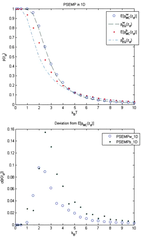
representing configurations that are one step away from the desired configuration. . . . . ... ... ... 58 3-9 Dynamic MC results using the solution to PSEMP for the 1D example

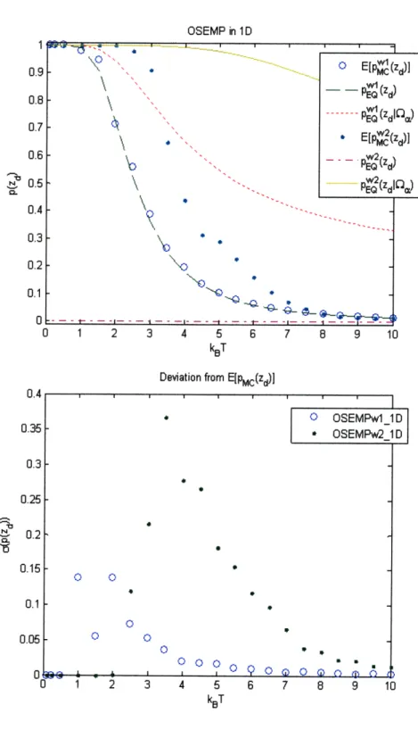
system compared to the Boltzmann probability distribution function. 61 3-10 Dynamic MC results using the solution to OSEMP for the 1D example

system compared to the Boltzmann probability distribution function. 64 3-11 The enumeration of all configurations in the ergodic component of the

1D example system. These configurations were used in the CEMP formulation. ... ... .. 67 3-12 Dynamic MC results using the solution to CEMP for the 1D example

system compared to the Boltzmann probability distribution function. 69 3-13 Dynamic MC results for the variability of the ensemble probabilities

using the solution to CSEMP for the 1D example system. ... . 70 3-14 The desired configurations for the two 2D example systems: (a) N =

7, V=16, (b) N=19, V=64 ... ... .. 72 3-15 The solution to the minimum tiling algorithm for both 2D example

systems. ... ... 72

3-16 The numbering of lattices sites from left-to-right and top-to-bottom for 2D square lattice systems. ... ... . . 75 3-17 Dynamic MC results using the solution to PSEMP for the 2D example

system (N = 7, V = 16). ... ... ... 76 3-18 Phase space energy distributions for PSEMP1w_2D and PSEMPlb_2D. 77 3-19 Dynamic MC results using the solution to OSEMP for the 2D example

3-20 Dynamic MC results using the solution to OSEMP for the 2D example system (N = 19, V = 64). . ... . . ... . . 80 4-1 Four representative configurations of the set of configurations with an

occupied lattice site 1. . ... ... 85 4-2 The multiresolution distribution of particles for the Dynamic Problem

solution ... . ... 86

4-3 The dynamic path that restricts the system to progressively smaller subsets of the system's phase space. . ... 88 4-4 Possible locations of point conditions for each stage of the dynamic

process. ... ... ... .. 89 4-5 Types of energy distributions that can result from solving EMP at

each stage of the dynamic process: (a) positive 6 separating the desired from the competing configurations; (b) negative 6 with the two sets of configurations overlapping; (c) zero 6; (d) negative 6 with the desired set of configurations subsumed in the energy range of the competing set of configurations. ... . ... 93 4-6 Two configurations belonging to 2 different components that portray

the difficulty in guaranteeing that 6 > 0 in the multiresolution EMP formulation. Using the well-forming point conditions, the level 1 com-peting configuration shown will have a lower energy than the level 1 desired configuration shown. . ... .... 93 4-7 The flowchart of the dynamic self-assembly process approach when the

same point condition locations are used in each process stage .... 96 4-8 A pictorial representation of the different regions of the probability of

achieving the desired state at a particular stage. Given changes in a particular system parameter, the system can transition from an ergodic to a nonergodic system, and vice versa. . ... 100 4-9 A view of the dynamic process at each stage, defined by the

4-10 Dynamic MC results for staying in the desired set of configurations for each stage of the dynamic process for the ID example system (N =

6,V= 16) ... ... . 102

4-11 Results from dynamic MC simulations of the dynamic self-assembly process for the 1D example system. . ... .. 103 4-12 The desired particle number distributions in the three stages of the

dynamic process for the 2D example system (N = 7, V = 16). ... . 105 4-13 The point condition locations analyzed for the 2D example system. . 106 4-14 Dynamic MC results for staying in the desired set of configurations for

each stage of the dynamic process for the 2D example system (N =

7, V = 16). ... ... ... 107 4-15 Results from dynamic MC simulations of the dynamic self-assembly

process for the 2D example system. ... . . . . . ... 109

B-i The desired configuration and point condition locations for another 1D example system (N = 5, V = 8). ... . . . 115 B-2 The desired configuration and point condition locations for another 2D

example system (N = 119, V = 1024). . ... 116 B-3 The barrier-forming point conditions and 23 well-forming point

List of Tables

3.1 EMP results for the 1D example system. . ... 65 3.2 Marginal values for the linear constraints using the OSEMP formulation. 65 3.3 EMP results for the 2D example system (N = 7, V = 16)... . . 73 3.4 EMP results for the 2D example system (N = 19, V = 64). ... 74 4.1 Initial guesses and generated point condition strengths for the 1D

ex-ample system ... ... ... ... 101

4.2 Initial guesses and generated point condition strengths for the 2D ex-ample system. ... . ... 105

Chapter 1

Introduction

The fabrication of structures with desired nanoscale geometric features is a core re-quirement for the manufacturing of future electronic, magnetic, and optical devices, composed of nanoscale particles or blocks of particles, e.g., nanoelectronic circuits, high-sensitivity sensors, molecular computers, molecular-scale factories, synthetic cells, adaptive devices (e.g., artificial tissues and sensorial systems, scalable plas-monic devices, chemico-mechanical processing, nanodevices and targeted cell ther-apy, human-machine interfaces at the tissue and nervous system level)[1]. The theory and practice of forming closely-packed 2-dimensional films and 3-dimensional ma-terials with desired periodic nanoscale geometries in an essentially infinite domain have advanced significantly during the last 10-15 years. For example, a large va-riety of self-assembled monolayers, leading to highly structured films on surfaces that provide biocompatibility, control of corrosion, friction, wetting, and adhesion, have been experimentally synthesized and theoretically analyzed[2_{]. These films are} viewed as possible precursors to nanometer-scale devices for use in organic microelec-tronics. However, their geometries are essentially periodic, which could constitute an important limitation. The features of phase-separated regions of block copoly-mers and blends are often of nanometer scale, periodic and dense, and can be ra-tionally designed through the judicious selection of the monomers, and the length and frequency of blocks in the polymeric chain(s)[3 , _{4]. Furthermore, templated} self-assembly techniques have been extensively developed to produce nanostructures with

desired geometries through the judicious selection of nanoparticles and features of the system environment. Examples include crystallization on template surfaces that determine the morphology of the resulting crystals[5_{] and crystallization of colloids} in optical fields [61. The templates could be physical (capillary forces, spin-coating, surface steps, and others), molecular (patterned self-assembled monolayers with spe-cific chemical functionalization of terminal groups), or electrostatic (localized charges on the surface of a substrate). The resolution of the structural features that can be achieved by template-based approaches depends on the spatial resolution of tem-plates. DNA-programmed placement using 2-dimensional DNA crystals as scaffolds, placement using electrophoresis, and focused placement, which uses focusing mech-anisms to guide the nanoscale particles to specific locations in the physical domain that are smaller in scale than the template guiding them, are additional approaches that have been extensively reviewed by Koh[7_].

Major challenges remain in two areas: (i) the fabrication of non-close-packed ma-terials with asymmetric structures, and (ii) creation of composite systems through the precise positioning of individual functional units. In both cases the fundamen-tal problem is how to place the individual elements (e.g., nanoparticles, nanowires, nanotubes, fragments of DNA, oligomers, proteins) at precise positions in a physi-cal domain so that they are connected to each other to form a complex structure of desired geometry and are also connected to the outside world with which they interact. As an example, let us use a lattice model to represent a system of N par-ticles within a system volume V. Figure 1-1 shows different categories of desired self-assembled structures for such a model system. Judiciously designed nanopar-ticles can self-assemble and form the periodic structures in Figure 1-1(a), but to form non-periodic nanostructures like those in Figure 1-1(b) external controls are needed to guide the self-assembly process. The size of the physical domains may be defined through a top-down fabrication technique such as photolithography[8 , _{91 or} nanoimprinting[10_{, 11, 12] and could produce domains with dimensions of '50nm or} larger. External controls, which may include electric or magnetic fields, chemical func-tionalizations, could be positioned through various top-down fabrication techniques,

e.g., 2 nm diameter electrodes made with electron beam lithography[1 3], carbon nan-otubes as electrodes (1-5 nm diameter)[1 4_{], etc. The particles may have charges,} dipoles, long-range and/or short-range interactions with each other, specific affinities (e.g., "patchy" particles[15 ], DNA molecules[16, 17, 181), etc. The resolution in the distribution of controls is limited by the physics of the fabrication technique. For example, electron beam lithography can generate arrays of electrodes 2 nm in diam-eter with about 20-50 nm between electrodesl13] . Thus, in selecting the location of external controls we must always conform with these physical constraints.

New approaches are needed to design and construct non-periodic and non- closed-packed nanostructures systematically, and this need defines the scope of the work presented in this thesis. More specifically, the following design questions are ad-dressed: (a) Static Problem: what are the optimal external controls so that the desired nanostructure is stable with a desired degree of robustness? (b) Dynamic Problem: how do we change the external controls over time in order to ensure that the desired final structure can be reached from any initial distribution of the particles in the physical domain? The first problem is addressed in Chapter 3, and the second problem in Chapter 4. However, before we can address these problems, we provide some background on statistical mechanics considerations (Section 1.1), lattice models for self-assembling particle systems (Chapter 2), and Monte Carlo (MC) simulation techniques (Section 2.2).

1.1

Statistical mechanics

Statistical mechanics is a probabilistic approach to the thermodynamic principles of chemical systems and is traditionally considered a molecular understanding of systems in the thermodynamic limit, i.e., N --+ c, V --+ oc, = v, where the specific volume v is finite. We cite here a few statistical mechanics textbooks[19 , _{20, 21, 22] that} provide an excellent background on the principles of this field.

The first law of thermodynamics states that both work and heat are forms of energy, and that the total energy is conserved. This is summarized by the fundamental

Periodic

,NME ME-M NoN

_

I I ....

mir ... -

M

--M

MENoM

(a)

Figure 1-1: The periodic nanostructures in (a) can be achieved through self-assembly of judiciously designed nanoparticles, but the non-periodic structures in (b) require external controls for guided self-assembly.

Non-periodic " ONNoM

ON,, M,,

SEEM.-MEMO

-SO~MEN

so0

mMMENNEmmE

"

NNEm

"

NNE MENE

MENEM

equation:

E= TS + J . x + p. N, (1.1)

where J represents generalized forces, e.g., pressure (-P), and x represents general-ized displacements, e.g., volume (V), and p is the chemical potential. This equation tell us that a system is fully specified by 3 variables, one from each term in the above sum. The most common system types, or ensembles, are the following: (1) N, V, E (microcanonical); (2) N, V, T (canonical); (3) p, V, T (grand canonical); (4) N, P, T (Gibb's canonical). These systems are equivalent in the thermodynamic limit, but this equivalency breaks down for finite systems (see Section 1.1.1). Hence, for nanoscale systems with finite N and V, each system type must be understood separately.

Thus far, we have described energy as a thermodynamic quantity. At the mi-croscopic level, we know that systems are composed of smaller constituents (e.g., particles, molecules, atoms), whose interactions and dynamics are reasonably well-understood in terms of more fundamental theories. At any time, t, the microstate of a system of N particles is described by specifying the position, q(t), and momentum, p(t), of all the system constituents. Thus, the microstate, m(t) = 1 f{qi(t),pi(t)}.

The classical energy function for a particle system at a particular microstate can be divided into separable potential and kinetic energy terms:

E(m) = EPE(q) + EKE(P), (1.2)

where it is assumed that the potential energy is only a function of position and the kinetic energy is only a function of momentum.

The model systems described in Chapter 2 specify N, V and T, and are there-fore canonical in nature. The probability distribution function (pdf) of a particular microstate, mj, in the canonical prescription is given by the Boltzmann equation:

where Z is called the normalizing partition function:

Z = e-3E(mk). (1.4)

k

Equation 1.3 is an ensemble probability, i.e., p(mj) represents the fraction of an ensemble of systems that are in microstate mj. It also represents the probability of finding a representative system in state mj after the system has reached equilibrium. The energy parameter, 0, essentially determines the "flow" of the system through phase space. The smaller the 0 value, the more accessible all states are to the system. Traditionally, / = 1/kBT. Because we assume that the kinetic and potential energy terms are independent from each other in Equation 1.2, we can split the Boltzmann pdf:

p(m) = p(p) - p(q) = Z;le - EKE(P) . Zq-le- EPE(q), (1.5)

where Z, and Zq are given by

Z= e-EKE(Pk), (1.6)

k

Zq =E e-)3EPE(qk) (1.7)

k

Analyzing only the Boltzmann pdf, we see that the most probable configuration(s) minimizes the energy E(m); configurations of equal energy are equally probable. Changing the random variable from microstate mr to energy, E(m) = :

p(c) = 3p(mk)6(E(mk) -) Z-I'e- (E(mk) -- ) = Z-1Q(c)e

-, (1.8)

k k

where Q(c) is simply the number of microstates with energy e. We define entropy as

Given this definition, Equations 1.8 and 1.9 can be used to give

p(E) = Z-1e- 3( - TS()) = Z-le - F(E), (1.10)

where F(e) = c - TS(e) is the Helmholtz free energy. Therefore, if we work in the energy space, it is the free energy that is minimized at equilibrium and the entropy that informs us of the degeneracy of a particular energy state.

The other ensembles are also important to analyze, especially since finite systems do not allow for ensemble equivalency. For example, one can imagine an open system with a particular volume, V, and temperature, T, but does not maintain the same particle number, N, in time. This grand canonical system prescription has important applications in open particle systems.

1.1.1

Thermodynamics of small systems

The fundamental laws of thermodynamics and their derivations from statistical me-chanics require that the system be in the thermodynamic limit. Under these circum-stances, the system parameters typically do not exhibit significant fluctuations. The following derivation portrays this principle.

Using the maximum-term methodll]9 , one can simplify Equation 1.4:

Z = e-OE(mk)= F() e--F(O) (1.11)

k {E}

where 6* is the energy state that minimizes F(e), i.e., the most probable energy state. This approximation holds true for systems in the thermodynamic limit (see Appendix A for the proof). The average energy can be computed as follows:

E = EE(mk)Z-le-E(mk) - nZ (1.12)

kIf energy, F = E we define an average free TS, where both energy and entropy are

also averages, then we can also use the following equation for the average energy:

- F & (\ F _ (pF)

E=F _{+ TS = F - T = -T} 2

)

- (1.13)

OT _{OT T ap}

Equations 1.12 and 1.13 tell us that

F = -kBTlog Z. (1.14)

In the thermodynamic limit, Equation 1.11 tells us that

F(E*) = -kBTlog Z. (1.15)

Hence, in the thermodynamic limit, the average energy state is also the most probable energy state. We can get an idea of how true this is by analyzing the variance in

energy, var(E) = E2 - 2:

var(E) = E2- E2 = Z- E2-E - Z- 2 Ee - E)

2 In Z 0E 0E

S02 Z= kBT2 = kBT2 .C, (1.16)

a02 0/3

where C is the heat capacity. The relative root mean square difference of the energy is given by

rms(E)= var(E) /kBT 2 .

rms(E) (1.17)

E E

The root mean square difference essentially is the average energy difference from the mean normalized by the average energy. Having a small value for this ratio means that the energy does not deviate much from its mean value. In the thermodynamic limit, the heat capacity and the system energy are extensive, i.e., (E, C) = O(N1),

which means

rms(E) = O (. (1.18)

Therefore, for a system in the thermodynamic limit, the root mean square difference is essentially nonexistent (for N = 0(1023), rms(E) = O(10-12)), and the most prob-able energy is the average energy. However, as we decrease N, as in biological and nanotechnological systems, fluctuations become significant.

Researchers are currently working on new theories, e.g., thermodynamics of small systems[2 3, 24], nonextensive thermodynamics[2 5], which account for phenomena that counter the classical laws due to finite system sizes. For instance, it has been shown that finite systems may violate the second law of thermodynamics[2 6 , the principles of extensivity and intensivity[2 7 , and ensemble equivalency[2 81. Mohaz-zabi and Mansoori[2 7] _{have shown that finite systems exhibit subextensivity, i.e.,} E, C - O(N), where A > 1. We can generalize Equations 1.17 and 1.18 as follows:

NB

rms(E) = O ) = =0 N . (1.19)

Ensemble equivalency has often been applied to problems which are difficult to solve under one set of thermodynamic conditions but easily solved under another set of conditions. For finite systems, such methods are no longer available. Statistical me-chanics, however, is not restricted to infinite systems and we utilize its basic principles that do not utilize the thermodynamic limit assumption.

1.1.2

Ergodicity considerations

Equations 1.3 and 1.10 both assume that the "flow" through phase space allows eventual access to any other state from any particular state. This is the ergodic

hypothesis, and is an important consideration. For the controlled self-assembling processes we discuss in Chapters 3 and 4, the externally imposed controls offer degrees

of freedom that can be used to decrease the volume of phase space accessible to the system, i.e., decrease the number of microstates accessible from any given microstate. Systems that exhibit such nonergodicity[2 91 _{are known as glassy systems[}3 0 , _{31] and} characteristically have rugged energy landscapes. As a result, transitioning between two ergodic subsets of phase space, separated by a large energetic barrier, is not very probable and requires either a sufficiently small /3 value or a sufficiently long period of time.

In questioning whether the behavior of a particular system is ergodic, one always needs to consider two aspects: (1) the time-scale of interest, and (2) the temperature of the system. Given a finite measurable time, many systems are effectively noner-godic and are therefore not properly described by the Boltzmann equation. Also, as one lowers the system temperature, the system may become trapped within energy wells, breaking system ergodicity. Spin glasses[3 0_{1 have become the model system for} the study of nonergodic behavior, which has found applicability in areas of research such as protein folding[3 2 , 331

A system with competing interactions exhibits "frustration". This phenomena describes the system's inability to satisfy all competing internal interactions, making a rough energy landscape with many local minima separated by high energy barriers. Given a sufficiently low temperature, i.e., below the glass transition temperature, or a finite time-scale, a system exhibits nonergodic behavior. However, one can analyze a nonergodic system's phase space Q, as a set of ergodic subsets, called components, where

Q = UQQ. (1.20)

A system which is in equilibrium within but not between components is referred to as being in quasiequilibrium, which describes a system trapped in a local minimum well. Because of the ergodicity within a component, one may use the Boltzmann equation

within each component:

e-E(mi)

Pa(m) i) e-E(mk) - Z-le-E(mi), (1.21)

ZMkECz~a E(mk)

where Z, is now the partition function of the ergodic component, a, and the sum over k is over all states in a with state mi being in a.

In the Static Problem, we require that the desired configuration be robust, i.e., once the system reaches the desired configuration, it stays in it. From a statistical mechanics perspective, this requirement implies that we want to maximize the prob-ability of the system being in the desired state and therefore minimize the desired state's energy compared to energies of all other accessible states. Under such condi-tions, the partition function is dominated by the desired state, leading to its increased probability, i.e., p(mdesired) --+ 1. This essentially means we have created a nonergodic system where the desired configuration is the only probable state in the accessible system component. These considerations form the basis of the problem formulation for the Static Problem (Chapter 3). Nonergodicity is also a desirable trait in the self-assembly process, where the desired configuration is the system's final equilib-rium state, because it reduces the total number of undesirable competing states. In Chapter 4, we propose a systematic restriction of phase space, starting with an er-godic system where all of phase space is accessible. At all times, the desired state is a member of the component the system is trapped in.

Chapter 2

Model systems

The model system we use to demonstrate our self-assembly design strategies is an isomorph of the Ising model[3 4] , the workhorse of statistical mechanics. We assume that the system particles do not rotate but simply translate throughout the discrete system volume. We also assume that the particles are indistinguishable and negatively charged with a charge equal to -1. Analyzing only the positional pdf, the potential energy function (note that we have dropped the subscript) is given by

V Nd

E(z) = Eet(z) + Eint(z) = ziHi,kSk + E i,jzj = zTHs + zTJz. (2.1)

i=1 k=1 i<j

The binary vector, z, represents the system configuration, where zi = 0 represents an empty lattice site and zi = 1 represents the presence of a particle. V is the system volume, i.e., the number of lattice sites, and Nd is the number of external fields (controls). The first sum, Eet, is the total energy imparted on the system by external fields, and the second sum, Eit, accounts for binary interactions between the system constituents (particles). Higher-order interaction terms may be included, if necessary. Because we are using a phenomenological model, we tend to simplify the system and focus on the most important contributors to the system behavior. The parameter Sk is the strength of external field k.

Many binary interaction potential energy models have the following form:

c(p)

c(P) f(P)(ri,Y) = ZiZy (2.2)

ij ij p i,j p

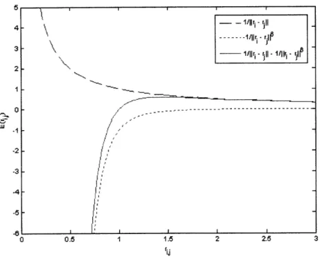
where rj is the positional distance between constituents i and j, and c is typically a fitted parameter used to match the model to experimental results. The larger the exponent, mp, the shorter the interaction range. For instance, the classic Lennard-Jones potential has an attraction interaction exponent, m = 6, whereas the Coulombic potential has an interaction exponent, m = 1. Figure 2-1 shows that Coulombic interactions are more long-range compared to the Lennard-Jones model for van der Waals attraction. Of course the total interaction energy is the sum of all short-and long-range contributions, shown in the above equation as a sum with the index p. Both types of interactions are important considerations in a self-assembly process; long-range interactions may be used to attract or repel system constituents within the system volume and short-range interactions may be used to define the local geometry of neighboring constituents. In this body of work, we consider particles interacting with both long- and short-range interactions.

The most basic external field potential function takes the following form:

Eext (z) = zEH₂,kSk - ZiCi,kSk, (2.3)

i,k i,k

where Ci,k is simply a constant. We may also introduce external fields that can take a basic form similar to the binary interaction potential above:

ext

()

(2.4)

i,k i,k p i,k p

Here, we introduce a distance parameter, ri,k, which represents the distance between lattice site i and external control k. We call this type of external field a point condition because the field originates at a point that is a certain distance away from each lattice site and influences the lattice site through a potential that is a function of

1I2 -- r II 0 1-- 1 2.5 I -// . .- - - -. . . . . .- -. . . . . . . . . -. 26 v~--1

2.1 Potential _{-2We take a more complicated} energy _{form for the} considerations_{interparticle interaction potential energy}

.4i

0 0.5 1 1.5 2 2.5 3

Figure 2-1: The long-range repulsive and short-range attractive interactions among the self-assembling particles.

that distance. Each point condition has a positional array and can be located within (internal point condition) or outside (boundary point condition) the system volume. The point condition locations and strengths are determined by solving the Static Problem (see Chapter 3). When sk is positive, the point condition k, in general, produces an energy well, and when sk is negative, k produces an energy barrier.

2.1

Potential energy considerations

In all of our examples, we utilize point conditions as a means of controlling the features of the potential energy landscape. More specifically, we use the external potential energy function in Equation 2.4 with p 1, 1) = -1 and ml = 1. This is

a simple phenomenological model for Coulombic charged interactions. The negative constant value simply represents the fact that we specify negatively charged particles. We take a more complicated form for the interparticle interaction potential energy

function, using Equation 2.2 with p = 1,2; (c,c) = (1,-1); and (ml, m2)

(1, 6). These parameter values represent a simple phenomenological model for long-range Coulombic charged repulsion and short-long-range van der Waals attraction. More specifically, we utilize the following overall potential energy function:

E = Eext +Eint = - zi + zz . (2.5)

ik i,k ij j ,3

For real systems, more complex interaction energy models will be required, but the above model serves as a phenomenological one.

2.2

Simulation techniques

Because we are working with a lattice model system and we are only analyzing the potential energy of a specific microstate, i.e., we are only looking at the system con-figuration space, we utilize Monte Carlo techniques[3 4, 35] to simulate our system. For a particle system of N particles in a finite volume V operated at a specific tem-perature T, one Monte Carlo simulation takes a representative system from an initial configuration to its stable equilibrium state. At equilibrium, the probability of being in a particular configuration state arrives at a limiting value, called the equilibrium probability. The evolution of the probability distribution in time is represented by the master equation:

Sp(z t) = _{[p(z, t)Wj' - p(z,}

_t)W1,

j#j

where p(zi, t) is the probability of being in state i at time t. The first term in the summation is the rate that the system arrives at state i from state j; Wji is the probability of transitioning from state j to state i. The second term is the rate that the system leaves state i. As the system approaches equilibrium, the above equation reaches a steady state, i.e., p(zj, t) -- p(zj). There are many ways that this equation can equal zero, but the most common approach is to impose detailed balance on the

system:

(2.7)

There are many choices for Wij that satisfy the above equation, the most famous of which is the Metropolis Monte Carlo scheme[3 6 ]_:

(2.8)

ij p (z ) }

Using the Boltzmann distribution equation for an ergodic phase space or an ergodic subset of phase space, this equation can be expanded:

W,j = min {1, e- (E(zj) - E(zi))} _(2.9)

The right-hand side of the above equation comes from comparing the two energy values, E(zi) and E(zy). If E(zi) > E(zj), then the minimum value is unity. If, however, E(zi) < E(zj), then the minimum value is the exponential term. To prove detailed balance, if E(zi) > E(zj),

Wj

)

p(zj)Wj_

p(zi),

As can be seen, detailed balance is satisfied. If E(zi) < E(zj), we can perform a similar analysis: Wij = e- (E (zj)- E (zj)) p(zi)Wij = p(zi)e-Th(E(zj)-E(z)) Se -3E(Zj). Wji = 1, p()W = p(zj), = e- E(zj ). (2.11)

This also satisfies the detailed balance criteria.

In standard Monte Carlo simulations of particle systems, the system is initialized at a particular state, z0o, and a sequence of one-step moves of individual particles are proposed and accepted using the acceptance probability in Equation 2.9, leading the system to equilibrium. The transition from the initial state to the equilibrium distribution of states may also serve as an approximation to the system's nonequilib-rium dynamics. However, if the system exhibits strong interaction potentials, defined by Unt and Uext, we may find that the system gets trapped in unphysical kinetic traps. For example, if two particles are located in neighboring lattice sites and there is a strong short-range attractive potential between them, then the likelihood of one particle moving one site away from its current location is very low. In essence, the system is trapped in an unphysical potential energy well. It is unphysical because a real system's potential energy surface would not include such a well; the two particles would simply move together in concert. The problem with the standard Monte Carlo approach therefore lies in the fact that it does not allow for movement of clusters of particles that are interacting through strong-range attractive potentials. Therefore, the Monte Carlo method we use throughout the self-assembly studies in Chapters 3 and 4 utilize the "virtual-move" Monte Carlo (vmmc) algorithm, developed by Whitelam and Geissler[3 71.

2.2.1

Dynamic Monte Carlo

Given a system of particles, the vmmc algorithm chooses a seed particle, i, and creates a cluster of linked particles, Ci, that moves together in concert. The same cluster of particles can be formed and moved in concert using multiple linkages with different seed particles. Similar to the detailed balance criteria above, the vmmc method satisfies superdetailed balance through the following equilibrium requirement:

p(zj)Wjkci- = p(zk)Wk-,jCic, V(i, j, k),

j

#

It is called superdetailed balance because it is specified over a specific linking between particles. More specifically,

= Wgenlc C -cckICi, (2.13)

where Wge" is the probability of proposing (i.e., generating) and moving from state zj to state zk, and Wacc is the probability of accepting the move from state zj to Zk. We can break down the first term as follows:

WjgkiC Pseed(Zj)Pdisplace(Ci; Zj -- Zk), (2.14)

where Pseed(zj) is _{the probability of choosing a seed particle in state zj and pdisplace(Cj; zj}

zk) is the probability, given a seed particle, of building Ci and moving it from state

zj to state Zk. This latter term can be broken down further to two factors:

Ci

Pdisplace(C; Zj + Zk)

J

-

{ mn}, {mn)j

The first product is the probability of not forming links between all the particles within Ci and all the particles that do not belong to Ci. Hence, the product over {mn}n, is the product over all particle pairs, m and n, that must not form in order to move from state zj to Zk. The second product is the probability of forming a specific

set of links between the particles that form the Ci cluster. From Equation 2.12, superdetailed balance now states that

p(zj)Wgen c-kCi = p(zk)Wgenj ₀. c j_]C, V(i, j, k), j $ k. (2.16)

This can be rearranged as follows:

_SajlCi p(Zj) Wgen "

T a m acc

f

There are many choices for Wja-cklC that satisfy the above equation. Whitelam and Geissler use the following form:

S min

1,

-ic lc Min _I Pseed(zj)

I{mn}k:3 1- Pmn(Zk z

fC

lImn)k 1 - pmn(Zj Zk) Pmn(Zj Zk) (2.18)

We can choose the seed particle from a uniform distribution, and therefore pseed(Zj) =

Pseed(Zk). The probability pmn(Zj - Zk) depends on the energy difference of the bond

between particles m and n before and after the seed particle is moved:

Pmn(Zj - Zk) = max {0, 1 - e-(Ej(m,n)-Ec(m,n)) }. (2.19)

The energy Ec(m, n) is the energy of the bond between a concerted move of particles m and n. Because the particles do not move relative to each other, this bond energy is identical at the beginning and end of the move. The energy EI(m, n) is the bond energy following an individual move of particle m without moving particle n.

Using the above derivations, the vmmc algorithm proceeds as follows:

Step 0: Start in state zj. Define the number of MC steps for the simulation.

Step 1: Select from a uniform distribution a seed particle, m, and a proposed translation.

Step 2: Find the particles, {n}, that interact with the seed particle. Link a given particle, n, to the seed particle with probability, pmn(zj - zk).

Step 3: Calculate pmn(zk -- zy).

Step 4: Perform Steps 2 and 3 recursively for each linked particle to form new links with each linked particle acting as the "seed".

Step 5: After no more possible links can be evaluated, update the position of the formed cluster using the proposed translation defined in Step 1.

Step 6: Evaluate the acceptance probability, and update the state of the system accordingly.

Step 7: Perform Steps 1-6 for the remaining MC steps.

All simulations in Chapters 3 and 4 use the vmmc algorithm to simulate both system equilibrium and nonequilibrium dynamics.

Chapter 3

The static problem

The static problem deals with maintaining the desired structure once it has been reached by the dynamic process. In essence, we assume that we have attained the desired geometry and our concern is to make this state robust. We are creating an ergodic component that consists of the just the desired state, and sufficiently large energy barriers keep the system inside this component. In order to shape the energy landscape for the creation of this ergodic component, we introduce system degrees of freedom in the form of externally-controlled point conditions. Each point condition has two parametric degrees of freedom: the location of the point conditions and their strength. The qualitative features of the energy landscape are defined by the location of the point conditions and their energetic characteristics, e.g., attractive or repulsive, while the quantitative features (the robustness) are determined by the point condition strengths.

We accordingly divide the Static Problem into two subparts: (a) the qualitative definition of the energy landscape through the specification of the point condition locations; (b) quantifying the robustness of the desired structure through the speci-fication of the strengths of the point conditions. Section 3.1 details how to system-atically place point conditions in order to qualitatively shape the energy landscape, introducing the minimum tiling algorithm for attractive and repulsive point con-ditions. Section 3.2 details the problem formulation and solution methodology for defining the strengths of the point conditions. To find the strengths we define and

solve the Energy-gap Maximization Problem (EMP), a combinatorially-constrained mixed-integer quadratic optimization problem. Section 3.4 provides examples that illustrate the qualitative and quantitative solutions of the Static Problem. Given the set of point conditions used, the system robustness can be quantified and the appro-priate operating system temperature can be found through simulation techniques. If the system robustness is such that the necessary operating temperature is imprac-tically low, we must introduce additional degrees of freedom to increase robustness. Section 3.3 details how we can use the EMP output to find the constraining features of the desired configuration and introduce the necessary degrees of freedom that en-ergetically influence these features.

3.1

Qualitatively shaping the energy landscape: the

minimum tiling approach

The qualitative features of the energy landscape are defined by the location of the degrees of freedom. The degrees of freedom we use are isotropic point conditions, which are attractive or repulsive in nature. Attractive point conditions introduce wells in the energy landscape, attracting the particles; repulsive point conditions introduce barriers, deflecting particles. Because the presence of two wells forms a barrier and vice versa, only one of these types (well- or barrier-forming) is needed to define the qualitative features of the energy landscape. However, when solving EMP, we may find that additional point conditions are needed to maintain a certain level of robustness. It is therefore necessary to solve EMP with both types of point conditions to see which is optimal in terms of two factors: (1) the total number of degrees of freedom needed, (2) the minimum distance between the degrees of freedom. Based on fabrication limitations, one can select which set of point conditions is more practical, while still maintaining the desired level of robustness for the desired structure.

To find the minimum number of well- and barrier-forming point conditions, we have formulated the minimum tiling algorithm below. For each point condition we

assign a tile that encompasses the local area that the point condition is intended to influence. Thus, the minimum number of tiles needed to cover the well- and barrier-forming regions determines the minimum number of attractive and repulsive point

conditions, respectively.

In our example systems, we restrict the point conditions to 3 types with respect to their locations. As shown in Figure 3-1, the point conditions can be on a lattice site, between two lattice sites, or between four lattice sites. The first two types apply to both the 1- and 2-D example systems while the third type applies only to the 2-D examples. One can consider the possible point condition locations as another system degree of freedom. The more types of point conditions (or, more generally, degrees of freedom) we provide the system, the less the number of point conditions we need, and vice versa. It is straightforward to see that for I-D systems (V = L) the number of possible point condition locations can be calculated for each type as follows:

No = L,

Nb = L + 1,

NP = N + N = 2L+1. (3.1)

In the same fashion, the number of possible point condition locations for 2-D square-lattice systems (V = L2) can be calculated as follows:

Npac = L2,

NP = 2(L + 1)L = 2L 2+2L,

Nf = (L+1)2

= L2 +2L+1,

N, = Na, + Nb + NC = 4L2 + 4L + 1. (3.2)

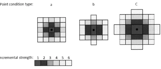
We only consider isotropic point conditions, and therefore each point condition's area of influence grows radially in all directions. The discretization of the system volume into lattice sites and the different locations of each point condition type cause their respective areas of influence to form different tile shapes. Figure 3-2 shows how

(a)

_(b)

_(c)

Figure 3-1: The three types of point conditions used in the example systems: (a) on a lattice site, (b) between two lattice sites, (c) between four lattice sites.

each type of point condition develops different tile shapes of increasing sizes. As a point condition's strength increases so does the area of influence it possesses. A point

condition's tile can only include lattice sites of one particular type, i.e., occupied sites for well-forming point conditions and unoccupied sites for barrier-forming point conditions. Therefore, when an incremental growth in the radius of a point condition's area of influence causes the inclusion of a lattice site of the opposing type, we know that the tile has reached its maximum size.

Given a desired lattice structure, the minimum tiling algorithm proceeds as fol-lows:

Step 1: Locate all possible point conditions of a particular type (well- or barrier-forming). N, = O(V).

Step 2: Grow each point condition's tile (defining the area of influence) to its maximum size. In other words, increment the radius of influence of each point condition until any further increase would include a lattice site of the opposing type.

Step 3: Eliminate all point conditions with null areas of influence. These point conditions are located in areas where the opposite point condition type is needed.

Step 4: Eliminate all point conditions with areas of influence completely sub-sumed by another point condition's area of influence. If the set of lattice sites

in the area of influence of point condition i is Si, we eliminate any point con-dition j where Sj C Si. If Sj = Si, then one point condition is chosen, which therefore allows for multiple solution sets of point conditions. We may eliminate multiple solutions by choosing the location that optimizes a particular system characteristic, e.g., maximizes the distance between point condition locations.

Step 5: Solve a set cover optimization problem with the remaining point con-ditions:

x

s.t. aijxi >

1,

xj e {0, 1}, (3.3)

where xi is a binary variable that takes a value of 1 if the point condition is kept and 0 if it is discarded. The parameter aij is a binary parameter that equals 1 if lattice site j is within the area of influence of point condition i, i.e., j is a member of i's tile, and 0 otherwise. The set of point conditions with xi = 1 represents the minimum set that covers all the lattice sites. After Step 4, the resulting point condition set is essentially all point conditions with independent sets of lattice sites in their areas of influence. Solving the set cover problem accounts for the fact that the union of multiple point condition tiles may subsume another point condition's area of influence, e.g., Si C Ulj,ihjlSj.

Step 6: Repeat Steps 1-5 for the other point condition type.

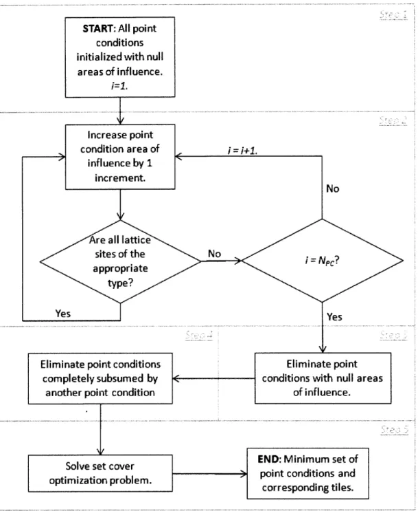
Figure 3-3 depicts the logical flowchart for Steps 1-5 of the minimum tiling algorithm. The set cover optimization problem in Step 5 is an hard problem with an NP-complete decision problem equivalent. If the number of point conditions considered is small enough, the set cover optimization problem can be solved for the minimum set. However, if the number of point conditions is too large, one must use an approximate algorithm, e.g., the greedy cover algorithm[3 8_{1. The greedy cover algorithm} sequen-tially chooses the point condition that covers the most number of lattice sites not yet

Point condition type: a b C

Incremental strength: 1 2 3 4 5 6

Figure 3-2: The geometry of tiles generated from the three types of point conditions defined in Figure 3-1.

covered by another chosen point condition.

The minimum tiling algorithm will output two sets of point conditions, the set representing the necessary well-forming point conditions to cover the occupied lattice sites and the set representing the necessary barrier-forming point conditions to cover the unoccupied lattice sites. These sets of point condition locations can be used to quantitatively shape the energy landscape, as described in Section 3.2.

3.2

Quantitatively shaping the energy landscape:

the energy-gap maximization problem (EMP)

Given the number of point conditions and their locations generated by the minimum tiling algorithm (Section 3.1), we must now guarantee that the desired configuration is robust, i.e., we want to maintain the desired structure given that the dynamic process allows us to reach the desired state. To do this we utilize the point condition strengths as our degrees of freedom. From Section 1.1, we may formulate this problem for a system in the Canonical prescription by simply maximizing its Boltzmann probability:

e-E(zd,s)

maxp(Zd, S) = max = max Z(s)-le- E ( d'S), (3.4)

START: All point

conditions initialized with null

areas of influence.

i=1.

Increase point

condition area of i= i+1.

influence by 1 increment.

No

Ere all lattice

sites of the No i

i = Npc?

appropriate type?

Yes _Yes

Eliminate point conditions Eliminate point

completely subsumed byI < conditions with null areas

another point condition of influence.

END: Minimum set of

Solve set cover

) point conditions and

optimization problem.

corresponding tiles.

Figure 3-3: The flowchart of the minimum tiling algorithm that generates the mini-mum number of well- or barrier-forming point conditions.

where s is the set of point condition strengths needed to calculate the system energy. We specify the partition function as that of the ergodic component, a, and the sum over j _{is over all configurations in a. Configuration zd is in a. From Section 1.1, we}

are also familiar with the ratio:

p(z 3 , s) = e-3(E(zis)-E(zj,s))

(3.5)

p(zj, s)

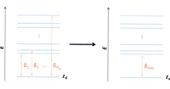
If E(zi, s) >> E(zy,s), this ratio approaches zero, and we know that state zj has a high probability. If E(zi, s) << E(zy, s), this ratio approaches infinity, and we know zi has a higher probability. Using this analysis, we see that we may analyze the equilibrium probability of being in a particular state versus any accessible competing states simply by looking at energy differences. We would like to minimize the energy of the desired state with respect to all competing configurations. To minimize the complexity of the problem, we may consider simply the competing configuration of minimum energy and the energy difference between this configuration and the desired configuration, see Figure 3-4. Using this approach, we may recast Equation 3.4 as a bilevel optimization problem:

max _{E*(s) - E(zd, s)}

sES

s.t. E*(s)= min E(z,s). (3.6)

zeno\{zd}

In this optimization formulation, which we call the Energy-gap Maximization Problem (EMP), the inner problem finds the configuration in the ergodic component, excluding the desired configuration, that minimizes the system energy. This configuration is then passed to the outer problem, where we maximize the energy difference between our desired configuration and the inner problem solution through the modification of the point condition strengths. A negative objective function value means that, given the set of point condition locations, the desired configuration cannot be the energy minimum and therefore is not the configuration within component a with the highest probability. In other words, there is at least one configuration with lower