Cell Reports, Volume23
Supplemental Information
Distinct Frequency Specialization for Detecting
Dark Transients in Humans and Tree Shrews
Human participants
10 20 30 40 50 30 50 70 90 40 Hz Light Dark 10 20 30 Modulation Depth 30 50 70 90 [% Correct] 24 Hz 10 20 30 30 50 70 90 15 Hz 10 20 30 30 50 70 90 11 Hz 10 20 30 30 50 70 90 8 HzTree Shrews
30 60 90 120 30 50 70 90 60 Hz 30 60 90 120 30 50 70 90 40 Hz 30 60 90 120 Modulation Depth 30 50 70 90 [% Correct] 24 Hz 30 60 90 120 30 50 70 90 15 Hz 30 60 90 120 30 50 70 90 11 Hz 30 60 90 120 30 50 70 90 8 HzA
B
Figure S1: Psychometric fits for the averaged response of the human participants and tree shrews
(related to Figure 2)
Psychometric functions fitted on the averaged responses of human participants (A) and tree shrews (B) to a
3 alternative forced choice (3AFC) task. The task was detecting a flicker stimulus among two equi-luminant
distractors. The psychometric functions were fitted separately for different frequencies and polarities. A
Gaussian sigmoid combined with a linear core (A) and partial linear fits (B) were used to fit the functions
(see supplemental experimental procedures for further details). Arrows indicate the modulation depth at
threshold (67% correct) for dark (blue) and light (green) flicker. The r2 of the linear fits in tree shrews for
light increments and decrements were as following: 0.683 and 0.959 for 7.5 HZ; 0.719 and 0.936 for
10.9 Hz; 0.663 and 0.888 for 15 Hz; 0.629 and 0.913 for 24 Hz; 0.571 and 0.889 for 40 Hz; and 0.309 and
0.729 for 60 Hz.
8 11 15 24 40
8 11 15 24 40
8 11 15 24 40
60
70
80
90
100
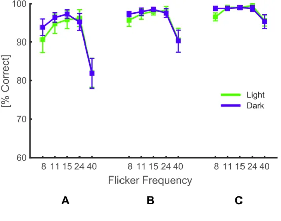
Figure S2: Average performance of human participants at supra-threshold
modulation depths
(related to Figure 2)
A, B and C show the average performance of human particiapnts at the 3, 2 and 1 highest
modulation depths tested in the experiment. While there is a clear main effect of frequency
at all three conditions, the repeated-measures two-way ANOVAs showed no significant
main effect of polarity or polarity x frequency interaction.
Average Performance
Flicker Frequency
[% Correct]
A
B
C
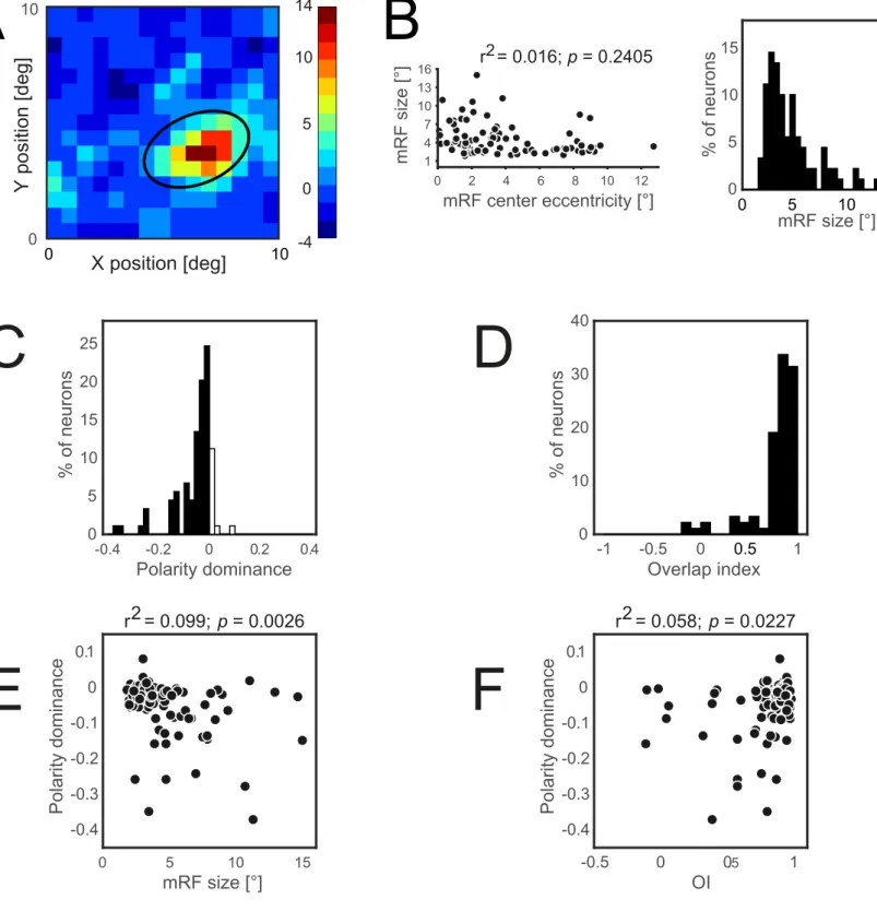
Light Darkr2 = 0.016; p = 0.2405 0 2 4 6 8 10 12 mRF center eccentricity [°] 1 4 7 10 13 16 mRF size [°] mRF size [°] 0 5 10 0 10 15 % of neurons
A
B
Figure S3: Receptive field mapping and
receptive field properties
(related to Experimental procedures)
A) receptive field (RF) of an example (off-center) unit mapped using sparse noise paradigm.
The colorbar shows firing rate (FR) relative to the average FR. The black oval denotes 2σ of
the RF. B) shows the correlation of the mRF size (left panel) and eccentricity and mRF size
distribution (right panel).
C) distribution of RFs based on the polarity dominance.
D) distribution of RFs’ overlap index (OI). The striate visual cortex of tree shrews is
overwhelmingly dominated by OFF-dominant neurons (~86%). Polarity dominance is also
significantly correlated with the mRF size (E) and overlap index (F).
0 10 0 5 10 15 -4 0 5 10 14
X position [deg]
Y position [deg]
-0.4 -0.2 0 0.2 0.4 Polarity dominance 0 5 10 15 20 25 % of neurons -1 -0.5 0 1 Overlap index 0 10 20 30 40 % of neurons 0 5 10 15 mRF size [°] -0.4 -0.3 -0.2 -0.1 0 0.1 Polarity dominance r2 = 0.099; p = 0.0026 -0.5 0 0.5 1 OI -0.4 -0.3 -0.2 -0.1 0 0.1 Polarity dominance r2 = 0.058; p = 0.0227C
D
E
F
0.5-50
0
50
100
TSI
0
5
10
15
20
% Neurons
0
50
100
TSI
-0.4
-0.2
0
Plarity dominance
r2 = 0.210; p = 0.0000
A
B
Figure S4: TSI (transient-sustained index) like measure and its correlation with
polarity dominance
(related to Experimental procedures and Figure 5)
A) shows TSI-like measure calculated using the ratio of the response to the dark flicker
from 51-100 ms after the latency of the stimulus (7.5 Hz) to the response from 1-50 ms.
Higher TSI values represent responses with more transient nature. The black line is the
mixed Gaussian fit on the distribution which shows a bimodal distribution with TSI
means of 84 and 35.9. B) shows the correlation of the TSI with polarity preference
suggesting units with stronger polarity dominance having more transient nature.
40.0 Hz 10 20 30 10 20 10 20 30 Trial 100 200 300 10 20 Spike Count 24.0 Hz 10 20 30 5 10 10 20 30 Trial 100 200 300 5 10 Spike Count 10.9 Hz 10 20 30 5 10 10 20 30 Trial 100 200 300 5 10 Spike Count 40.0 Hz 10 20 30 10 20 10 20 30 Trial 100 200 300 10 20 Spike Count 24.0 Hz 10 20 30 10 20 10 20 30 Trial 100 200 300 10 20 Spike Count 10.9 Hz 10 20 30 10 20 10 20 30 Trial 100 200 300 10 20 Spike Count Time [ms] Time [ms]
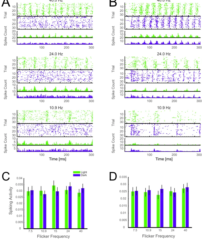
Figure S5: Response of two example units to light and dark flicker and normalized baseline spiking activity
(related to Figures 5 and 6)
A
B
Spiking Activity
Flicker Frequency
Flicker Frequency
7.5 10.9 15 24 40 0 0.005 0.01 0.015 0.02 0.025 0.03 0.035C
D
7.5 10.9 15 24 40 Light Dark 0 0.005 0.01 0.015 0.02 0.025 0.03 0.035 0.04Figure S5: Response of two example units to light and dark flicker and normalized baseline spiking activity
(related to Figures 5 and 6)
Raster plots of two example units representing spiking of neurons in response to light (green) and dark (blue)
flicker. The unit on the left (A) is ON-dominant and the unit on the right (B) is OFF-dominant. Each tick
represents one frame of monitor at baseline level with bold ticks representing the transients with luminance
increment (green) or decrement (blue). The plots under each raster plot show spike time histogram. C) depicts
pre-trial baseline activity 15 ms before the response. A repeated-measures two-way ANOVA showed no main
effect of frequency or polarity suggesting that neurons were at a similar level of light adaptation at the beginning
of the trials. D) shows the baseline activity during the last 25 ms of the interstimulus interval following each
trial. Since trials were randomized, this figure shows post-stimulus baseline following different conditions.
A repeated-measures two-way ANOVA demonstrated no main effect of polarity or frequency ensuring that
different conditions do not induce different levels of light adaptation in this experimental design.
PSTH
Flicker Frequency Flicker Frequency
7.5 10.9 15 24 40 0.4 0.5 0.6 0.7 0.8 0.9 1
Normalized spiking activity
Normalized spiking activity
OFF DOMINANT
ON DOMINANT
cycle = 1 Light Dark 7.5 10.9 15 24 40 0.4 0.5 0.6 0.7 0.8 0.9 1 cycle = 3 cycle = 1 cycle = 3A
C
Figure S6: Normalized spiking responses and response latencies of OFF and ON dominant
neurons to individual transients
(related to Figures 6 and 7)
A) represents the responses of OFF dominant units to the first (left) and third (right) cycles of the trials. There is
a main effect of polarity (p < 0.05) but not frequency during the first cycle. During the third cycle, there are main
effects of both polarity (p < 0.001) and frequency (p < 0.0001). B) represents the responses of ON dominant
neurons to the first and third cycles of the trials (left and right panels respectively). While a general trend pointing
to an increased activity in response to light flicker compared to dark flicker is seen, there is no significant effect of
polarity or frequency in either cycle 1 or cycle 3. Lower number of ON dominant cells can be a reason for the lack
of statistical significance. C) depicts the response latency of OFF dominant units to the first (left) and third cycles
(right). The latency of OFF units resembles the latency of overall population and show a very robust advantage for
dark flicker. D) ON units show no significant difference between response latency to dark and light flicker in either
first (left) or third (right) cycle though a trend for lower latency to the light flicker is seen at some frequencies.
7.5 10.9 15 24 40 0.4 0.5 0.6 0.7 0.8 0.9 1 7.5 10.9 15 24 40 7.5 10.9 15 24 40 7.5 10.9 15 24 40 7.5 10.9 15 24 40 7.5 10.9 15 24 40 0.4 0.5 0.6 0.7 0.8 0.9 1
B
D
PSTH Latency
Flicker Frequency Flicker Frequency
22 24 26 28 30 32 34 36 Latency [ms] Latency [ms] 22 24 26 28 30 32 34 36 22 24 26 28 30 32 34 36 22 24 26 28 30 32 34 36
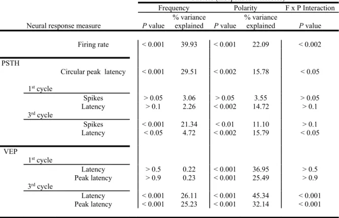
Table S1: summary of statistics on different measures of neural signals and their timing (related to Figures 4 -7)
Factors (independent variables)
Frequency Polarity F x P Interaction Neural response measure P value
% variance explained P value % variance explained P value Firing rate < 0.001 39.93 < 0.001 22.09 < 0.002 PSTH
Circular peak latency < 0.001 29.51 < 0.002 15.78 < 0.05 1stcycle Spikes > 0.05 3.06 > 0.05 3.55 > 0.05 Latency > 0.1 2.26 < 0.002 14.72 > 0.1 3rdcycle Spikes < 0.001 21.34 < 0.01 11.10 > 0.1 Latency < 0.05 4.72 < 0.002 15.79 < 0.05 VEP 1stcycle Latency > 0.5 0.22 < 0.001 36.95 > 0.5 Peak latency > 0.9 0.23 < 0.001 25.49 > 0.9 3rdcycle Latency < 0.001 26.11 < 0.001 45.34 < 0.001 Peak latency < 0.001 25.23 < 0.001 32.14 < 0.001
All the p values are the results of two-way ANOVAs with repeated measures in both factors (i.e. frequency and polarity). % variance explained represents the percentage of the total variance in the dependent variable (different neuronal signal measures) associated with either frequency or polarity after the effects of individual differences among units or sites have been removed. Latency in the PSTHs and VEPs refers to the timestamp that the respective neural response starts. Peak latency in the VEPs refers to the timestamp of the peak activity. F x P Interaction denotes Frequency x Polarity Interaction. p values less than 0.001 were not further categorized into smaller values.
Supplemental experimental procedures
All experimental procedures were conducted in accordance with the applicable Swiss and European regulations and were approved by the veterinary office of the canton of Fribourg.
Behavioral experiments
Nine human participants (5 males) including two authors (AK and FM) and six female tree shrews (Tupaia
belangeri) participated in behavioral experiments. Both species detected a flickering stimulus among two
equi-luminant distractors. Equi-equi-luminant distractors had the same time-averaged luminance as the target flickering stimulus. Stimuli presentation, reward delivery, behavioral control and collection of responses and reaction times were controlled by custom written MATLAB codes using Psychtoolbox 3 (Brainard, 1997). The visual stimuli were generated by introducing transient impulses of light increment or decrement from a mid-gray background at different frequencies and different modulation depths (Figure 1) and were presented on a gamma-corrected cathode ray tube (CRT) monitor. On every trial, a flickering stimulus, with particular values of three independent variables (flicker frequency, modulation depth, and polarity), was presented at a randomly selected location (the target location) and two equi-luminant distractors were presented at the remaining two locations. The refresh rate and average luminance of the monitor were held constant at 120 Hz and 36 cd/m2, respectively. Human
participants used a modified keyboard to report the correct target (50 cm distance) and completed 2700 trials across three sessions on three different days. The participants were free to choose the target as soon as they perceived a flickering stimulus among the presented stimuli.
The body weights (165 – 225 g) of tree shrews were monitored twice a week, which ensured the well-being of animals as the weight fluctuation between different days did not exceed 4g. The animals were food restricted every evening at 7 PM (these animals are diurnal) and the experiments were performed during the morning after 9 AM. Free access to food was provided to animals half an hour after the end of the experiments till 7 PM. During the weekends, there was at least one day with no experiment and therefore there was no food restriction. The animals had uninterrupted free access to water except during the experimental sessions. Tree shrews were extensively trained to detect a flickering stimulus from equi-luminant distractors by nose poking in the correct hole (Figure 1) in a custom-made box. Tree shrews were free to navigate within the box and were connected to a smaller nesting box through a tube and therefore could leave the experimental box to the nesting box whenever they decided to end the session’s trials. Although the animals were food restricted, the ability of tree shrews to self-terminate the sessions ensured that the tree shrews were not forced to perform trials at the end of the sessions after getting satiated and losing motivation. The levels of modulation depth were adjusted for tree shrews’ performance and due to their higher flicker fusion frequency, an additional level of frequency (60 Hz) was added to the five levels of frequency tested in human participants. The correct detection resulted in the delivery of two reward pellets in a reward magazine opposite of the stimulus presentation side. Incorrect responses were alerted by a beep and longer inter trial interval (6 s). The reward pellets were 45 mg raspberry-flavored food reinforcement pellets (P. J. Noyes). The distance between the reward magazine and the stimulus presentation screen was 38 cm and each hole had a dimeter of 6.5 cm subtending 9.7° of visual field. Note that
the animals were freely moving while performing the task and therefore the stimulus size was varying with the movement of the animals. For training, the flickering target stimulus was initially accompanied with two dark stimuli so that the animals could detect the target based on a large contrast difference. The luminance of the distractor was increased progressively during several steps as the animals surpassed the threshold performance of 65% for two consecutive days at each stage. Once the luminance of the distractor reached to the target
luminance, after several days of further training, the test phase started. Each animal was tested during many sessions (42 to 74) and each session consisted of 80 to 120 trials. All variables were randomized during test sessions. The 80 to 120 trials per session resulted from the ability of the animals to terminate the sessions at their free will. We fitted psychometric functions (cumulative Gaussian; Figure S1A) using constrained maximum likelihood and bootstrap inference by means of the psignifit toolbox (Wichmann and Hill, 2001a, b). For the analysis of tree shrew performance several sigmoid psychometric functions (including raw data and some log transformations) proved not to be robust in representing data. This is also visually clear that the data points do not resemble a sigmoid function at least for some frequencies. Therefore, we used linear regression (Figure S1B) for the initial segment of the data as the response pattern showed an initial sharp rise followed by a plateau. The criteria to include data points were as following. At least one point above the threshold had to be included (otherwise the behavioral relevance would be obscure) and to avoid underestimating the threshold (i.e.
overestimating sensitivity) at performance level around the threshold, the next data point was also included if it’s difference with the preceding data point was less than 5 (%). The non-parametric estimation of the sensitivity based on the area under the response curve corroborated the reliability of the threshold estimation based on the linear regression.
Electrophysiological recording and data analyses
Before the experiments, adult tree shrews (n = 7) were anesthetized with ketamine (100 mg/kg; im) followed by an injection of atropine (0.02 mg/kg; im) to prevent mucus secretion. The anesthesia was maintained with isoflurane (0.5 – 1.5%) delivered through artificial respiration as the animals were tracheotomized and a local anesthetic was also used during the surgery. All vital signs were carefully monitored during the experiment. An atropine drop was applied on both eyes for pupil dilation and contact lenses were placed on the eyes to avoid corneal drying. A small craniotomy removed part of the skull over V1 and two tungsten electrodes (500 μm apart, Impedance: 1 MΩ) were inserted into the brain using a remotely controlled hydraulic wheel. The recording sites were histologically confirmed by inducing a lesion at multiple sites at the end of recording sessions. Electrophysiological signals were amplified by a RA16PA Medusa preamplifier and were filtered and digitized by a RZ5 Biomap processor (Tucker-Davis Technologies, Alachua, FL). The signal was sampled at 24.4 KHz and was concurrently high-pass filtered at 300 Hz and low-pass filtered at 100 Hz. Action potential waveforms were recorded by thresholding the high-pass filtered signal and were sorted offline. The low-pass filtered signal was down-sampled at 1 KHz and contained LFPs. In each recording site, we analyzed signals from either of the electrodes and not both electrodes simultaneously. This limitation was imposed because two electrodes could be moved only together and not independent from each other which reduced the chances of simultaneous recording of well-isolated neurons. The stimulus presentation screen was placed at a 30 cm distance from the animal subtending ~60° of visual field. The stereotaxic frame could be rotated on a metallic
base and could be locked at every 30° allowing us to stimulate neurons with higher eccentricities and with receptive fields (RFs) outside the central field. RF of each site was mapped using sparse noise paradigm (for details, see: Poirot et al., 2016). Briefly, a large area including the putative receptive field location was determined by moving a black bar generated by graphic software at different orientations while advancing the electrodes via a micro-drive. The neuronal responses were visualized on the computer monitor and could be heard through a speaker. Whenever neuronal activity was clearly distinguishable from the background noise, sparse noise paradigm was presented at an area including the putative RF location. The paradigm consisted of full modulation black and white “dots” that were presented on an invisible 17*17 tile-wide grid. The grid covered 10*10° of visual field and each dot was presented on 2*2 tiles in the grid. Therefore, each tile of the grid was stimulated by four unique stimulus of each polarity. The paradigm was repeated five times. Whenever most of the tiles in the grid were stimulated suggesting a big RF, the paradigm was repeated on a grid covering 20*20° of visual field. Reverse correlation of sparse noise stimulus with spike trains from +20 to +100 ms since the stimulus onset was used to estimate RF size and location (Poirot et al., 2016; Veit et al., 2014). RF size and center was estimated by fitting the time-averaged response map with an oriented two-dimensional Gaussian function (Veit et al., 2014) resulting in an oriented ellipse. The fitting was performed separately for responses evoked by black and white dots to account for OFF and ON centers of the RF, respectively. The area from the center of the ellipse that contains 95% of the response (i.e. 2SD) was considered as mRF of the RF and the larger axis of the ellipse was considered as representative of the RF size. Furthermore, we computed functional
properties of the RFs, namely the extent of the overlap between two subfields and polarity preference. The overlap between two subfields was computed using the following formula:
OI = (2σwhite + 2σblack - Δµ)/( 2σwhite + 2σblack + Δµ)
Where OI refers to overlap index, σ denotes mean bi-dimensional spatial spread of the RF size calculated using sparse noise stimuli and Δµ is the Euclidean distance between the centers of the two subfields (Kagan et al., 2002; Poirot et al., 2016; Schiller et al., 1976; Veit et al., 2014). Polarity dominance was also calculated by a log ratio of the peak response of ON to the peak response of OFF subfields. Negative values signify dark preference (OFF dominance) and positive values signify light preference (ON dominance). The visual stimuli identical to those used in behavioral experiments were presented to the minimal RF of each recording site in randomized order. All frequencies were presented to all neurons. Single units were identified by sorting spikes according to the area below the spike waveform (i.e. energy) and interspike intervals. Custom written and built-in MATLAB functions were used to analyze data. The peri-stimulus time histograms (PSTHs) were estimated from the spike times, by time locking the signal to the onset of each stimulus. To calculate the neuronal response to each individual transient within each trial, a segment of signal (PSTH) was scanned starting from the first timestamp corresponding to the respective transient’s onset and the first two points (1 ms bins; no smoothing) that passed the threshold was marked as the neuronal response onset and used to calculate the response latency (Figure 5B). The threshold was the sum of the mean baseline response plus 3SD. All timestamps above the threshold within a time window of 13 ms after the response onset were summed after subtracting the baseline activity and
considered as the neuronal response for the respective transient.
Our stimuli were not suitable for classifying the neurons based on the transiency of their response since these stimuli were transient by nature whereas typically continuous flash light stimuli (Lu and Petry, 2003; Norton et
al., 1985) are used to estimate transient-sustained index (TSI). However, we estimated TSI-like (pseudoTSI) measure by comparing the late response to the early response following the flicker frequency of 7.5 Hz which had the longest cycle. This measure was calculated according to the following formula:
pseudoTSI = 100 – 100*( Rl / Re)
where Re and Rl represent early (1-50 ms since response onset) and late (51-100 ms) response of the neurons.
Neuronal responses to dark flicker showed a bimodal distribution of this measure (Figure S4A). While the measure that we calculated cannot be directly compared to Lu and Petry (2003) study due to differences in the stimuli, a mixed Gaussian model fit showed pseudoTSI means of 84 and 35.9 which closely corresponds to the findings of Lu and Petry (2003). Furthermore, as shown in figure S4B, pseudoTSI measure is correlated with polarity dominance such that the transiency nature of the neurons increases with stronger polarity dominance. After a short period of baseline recording, visual stimuli identical to those used in behavioral experiments were presented to the RF of the units. Flicker stimuli were generated by a combination of three variables: frequency (7.5, 10.9, 15, 24, and 40 Hz), Modulation depth (10, 40, 70, 100%) and polarity (+1 and -1). Each unique stimulus lasted 550 ms followed by a 58 ms intertrial interval and was presented ten times in a randomized order.
Statistical analysis
In this study, we used repeated measures analysis of variance (ANOVA) and post-hoc tests, non-parametric Wilcoxson signed rank test, bootstrap analysis, Rayleigh test for circular uniformity and aligned rank transform for non-parametric factorial analyses. The latter test is a non-parametric analysis for multi-factor data and resembles ANOVA procedures (Wobbrock et al., 2011). This test was conducted using open-source statistics software R and MATLAB functions were used for all other statistical analyses.
Supplemental references:
Brainard, D.H. (1997). The Psychophysics Toolbox. Spat Vis 10, 433-436.
Kagan, I., Gur, M., and Snodderly, D.M. (2002). Spatial organization of receptive fields of V1 neurons of alert monkeys: comparison with responses to gratings. J Neurophysiol 88, 2557-2574.
Lu, H.D., and Petry, H.M. (2003). Temporal modulation sensitivity of tree shrew retinal ganglion cells. Vis Neurosci 20, 363-372.
Norton, T.T., Rager, G., and Kretz, R. (1985). ON and OFF regions in layer IV of striate cortex. Brain Res 327, 319-323.
Poirot, J., De Luna, P., and Rainer, G. (2016). Neural coding of image structure and contrast polarity of Cartesian, hyperbolic, and polar gratings in the primary and secondary visual cortex of the tree shrew. J Neurophysiol 115, 2000-2013.
Schiller, P.H., Finlay, B.L., and Volman, S.F. (1976). Quantitative studies of single-cell properties in monkey striate cortex. I. Spatiotemporal organization of receptive fields. J Neurophysiol 39, 1288-1319.
Veit, J., Bhattacharyya, A., Kretz, R., and Rainer, G. (2014). On the relation between receptive field structure and stimulus selectivity in the tree shrew primary visual cortex. Cereb Cortex 24, 2761-2771. Wichmann, F.A., and Hill, N.J. (2001a). The psychometric function: I. Fitting, sampling, and
goodness of fit. Percept Psychophys 63, 1293-1313.
Wichmann, F.A., and Hill, N.J. (2001b). The psychometric function: II. Bootstrap-based confidence intervals and sampling. Percept Psychophys 63, 1314-1329.
Wobbrock, J.O., Findlater, L., Gergle, D., and Higgins, J.J. (2011). The aligned rank transform for nonparametric factorial analyses using only anova procedures. In Proceedings of the SIGCHI Conference on Human Factors in Computing Systems, ACM, ed. (Vancouver, Canada).