Incentives to Learn Calibration : a Gender-Dependent Impact

(1)

HAL Id: halshs-00348826

https://halshs.archives-ouvertes.fr/halshs-00348826

Submitted on 22 Dec 2008

HAL is a multi-disciplinary open access

archive for the deposit and dissemination of sci-entific research documents, whether they are pub-lished or not. The documents may come from

L’archive ouverte pluridisciplinaire HAL, est destinée au dépôt et à la diffusion de documents scientifiques de niveau recherche, publiés ou non, émanant des établissements d’enseignement et de

Incentives to Learn Calibration : a Gender-Dependent

Impact

Marie-Pierre Dargnies, Guillaume Hollard

To cite this version:

Marie-Pierre Dargnies, Guillaume Hollard. Incentives to Learn Calibration : a Gender-Dependent Impact. 2008. �halshs-00348826�

(2)

Documents de Travail du

Centre d’Economie de la Sorbonne

Maison des Sciences Économiques, 106-112 boulevard de L'Hôpital, 75647 Paris Cedex 13

Incentives to Learn Calibration : a Gender-Dependent Impact

Marie-Pierre DARGNIES, Guillaume HOLLARD

(3)

Incentives to Learn Calibration: a

Gender-Dependent Impact.

Marie-Pierre Dargnies

∗

and Guillaume Hollard

†

December 2008

∗_{Paris School of Economics, Université Paris 1 Panthéon-Sorbonne, CES 106-112}

boule-vard de l’Hopital 75013 Paris. Tel:(0033) 1 44 07 82 13. Fax: (0033) 1 44 07 82 31. E-mail: marie-pierre.dargnies@univ-paris1.fr

(4)

Abstract

Miscalibration can be defined as the fact that people think that their knowledge is more precise than it actually is. In a typical miscalibration experiment, subjects are asked to provide subjective confidence intervals. A very robust finding is that subjects provide too narrow intervals at the 90% level. As a result a lot less than 90% of correct answers fall inside the 90% intervals provided. As miscalibration is linked with bad results on an exper-imental financial market (Biais et al., 2005) and entrepreneurial success is positively correlated with good calibration (Regner et al., 2006), it appears interesting to look for a way to cure or at least reduce miscalibration. Previ-ous attempts to remove the miscalibration bias relied on extremely long and tedious procedures. Here, we design an experimental setting that provides several different incentives, in particular strong monetary incentives; i.e. that make miscalibration costly. Our main result is that a thirty-minute training session has an effect on men’s calibration but no effect on women’s.

Résumé

On désigne par l’anglicisme "miscalibration" le fait que les individus pensent que leur savoir est plus précis qu’il ne l’est en réalité. On mesure typiquement la miscalibration en demandant aux sujets de fournir des inter-valles de conﬁance à 90% pour une série de questions. Or, de nombreuses études (voir Lichtenstein and Fischhhoﬀ (1977) pour une revue de littéra-ture) montrent que le taux de réponses correctes appartenant aux intervalles à 90% fournis est toujours bien inférieur à 90%. On parle alors de miscal-ibration dans la mesure où les individus fournissent des intervalles à 90% trop étroits. Les liens existant entre la miscalibration et de mauvaises per-formances économiques (Biais et al. (2005), Regner et al. (2006)) expliquent l’intérêt pour les économistes d’étudier ce biais.

Notre protocole expérimental vise à réduire la miscalibration par le biais d’incitations directes, notamment monétaires. Notre résultat principal est que nos incitations ont un eﬀet sur la calibration des hommes, ceux ayant suivi notre entrainement fournissant des intervalles plus larges, mais aucun eﬀet tangible sur celle des femmes.

JEL Codes: D81, C91.

(5)

1 Introduction

In the past decades Economists and Psychologists documented a long list of biases , i.e. substantial and systematic deviations from the predictions of standard economic theory 1_{. Many economists will argue that these biases}

only matter if they survive in an economic environment. In other words, if correct incentives are provided subjects should realize that they are making costly mistakes and then change the way they make such decisions in further decision tasks. In this paper we test this claim regarding a particular bias, namely miscalibration. We then create an experimental setting that provides a lot of incentives (decisions have monetary consequences, successful others can be imitated, feedbacks are provided, repeated trials are used, etc). Fi-nally, we test in a subsequent decision task whether subjects still display some miscalibration.

What is miscalibration and why is it important to economists? Calibration is related to the capacity of an individual to choose a given level of risk. In a typical experiment designed to measure miscalibration, subjects are asked to provide subjective confidence intervals. For example, if the question is "What was the unemployment rate in France for the first trimester of 2007?" and the subject provides the 90% confidence interval [7%,15%], it means that the subject thinks that there is a 90% chance that this interval contains the correct answer. A perfectly calibrated subject’s intervals should contain the correct answer 90% of the time. In fact, a robust finding is that almost all subjects are miscalibrated. On average, 90% subjective confidence intervals only contains the correct answer between, say, 30% and 50% of the time 2_{. Glaser et al. (2005) found an even stronger miscalibration using}

professional traders.

Miscalibration is a bias having important economic consequences, since miscalibrated people suﬀer losses on experimental markets (Bonnefon et al., 2005, Biais et al., 2005). Furthermore, it is likely that such a pathology aﬀects the behavior of real traders acting on real markets. Therefore, it does make sense for economists to try to reduce miscalibration and to study the

1

A list of almost a hundred of such biases can be found at http : //en.wikipedia.org/wiki/List_of_cognitive_biases

2

see Lichtenstein and Fischhhoff (1977) for a survey and (Klayman et al., 1999) for variables that affect miscalibration

(6)

best incentives to do so.

Lichtenstein and Fischhoﬀ (1980) attempted to reduce miscalibration by providing subjects with feedback on their performance. They proved that 23 sessions, each lasting about an hour, were required to substantially im-prove subjects’ calibration. Several other psychologists have used various techniques to reduce miscalibration (Pickhardt and Wallace, 1974, Adams and Adams, 1958), with little success so far. Miscalibration thus appears to be a very robust bias.

This paper proposes to provide a maximum of incentives to reduce mis-calibration. The main result is that our experimental setting succeeds in reducing overconﬁdent miscalibration but only for males.

The remainder of the paper is organized as follows. Section 2 presents the experimental design. Section 3 presents the results and section 4 discusses them. Finally, Section 5 provides some concluding remarks.

2 Experimental design

The measure of miscalibration and associated overconﬁdence relies on a now standard protocol. Subjects have to provide 90% subjective conﬁdence inter-vals for a set of 10 quiz questions. On average, perfectly calibrated subjects should catch the correct answer 9 times; if this is not the case, they are miscalibrated. 3 _{The subjects are asked to estimate their hit rate. The}

difference between their estimated hit rate and their actual one is a classical measure of overconfidence. This protocol will thus serve as a benchmark for measuring miscalibration and overconfidence in our experiment.

The experimental subjects were divided into two groups. The subjects of the ﬁrst group attended a training session and then performed a baseline treatment aiming at measuring their miscalibration according to the stan-dard protocol. The principle of this training session is to oﬀer a whole set of experimental incentives that enhance learning (monetary incentives, tourna-ment, feedback, loss framing). The second group, the control group, performs the baseline treatment only.

3

Note that we cannot say of a single subject who only catches the correct answer in his 90% intervals, say, 6 times out of 10 that he is miscalibrated. Nevertheless, we can say of a population of subjects for which on average 6 correct answers out of 10 belong to the 90% intervals provided and with no subject catching 9 correct answers or more that it is globally miscalibrated.

(7)

At first glance, testing the effect of incentives seems possible by simply providing incentives for the basic miscalibration task used as a benchmark. This seems natural but cannot be implemented since there is no simple in-centive scheme that rewards correct calibration. Think, for example, of an incentive scheme that would pay a high reward if the difference between the required percentage of hit rates, say 90%, and the actual hit rate (measured over a set of 10 questions) is small. A rational subject can use very wide intervals for 9 questions and a very small one for the remaining question. He is thus certain to appear correctly calibrated, while he is not. Cesarini et al. (2006) chose to provide incentives for the evaluation of the calibration task only (how many correct answers belong to the intervals provided by the subject and by his peers) and made miscalibrated subjects go through the task again. We chose to consider a task similar to the calibration task in which we can provide the necessary incentives. This task, described in the following section aims at making the subjects realize they have a hard time calibrating the level of risk they wish to take. After having completed this training task, subjects have to complete a standard calibration task for which we only provide incentives for the following evaluation of how subjects did in the calibration task as in Cesarini et al. (2006). A control group who did not go through the training task also completed the calibration task to enable us to measure the effect of the training task.

2.1 The training period

In the training period, the participants were asked to answer a set of twenty questions: ten questions on general knowledge followed by ten questions on economic knowledge.

The set of questions used in the training period was composed of ten questions some of which were used in Biais et al. (2005)’s experiment plus 10 questions on economic culture. Half of the subjects had to answer the 20 questions in a given order, the other half saw the questions in reverse order. This enabled us to check for learning eﬀects during the training period.

In this training period, the subjects were provided with a reference in-terval for each question that they could be 100% sure the correct answer belonged to. Subjects had to give an interval included in the reference inter-val. Each player received an initial endowment of 2000 ECUs (knowing that they would be converted into euros at the end of the experiment at the rate of 1 euro for 100 ECUs) before beginning to answer the questions but after

(8)

having received instructions. They were told that 100 ECUs were at stake for each one of the twenty questions resulting in a loss framing. The payoﬀs are expressed in experimental currency (ECU). The payoﬀ rule applied for each question was the following. :

payment =         

−100 ∗ _{width of the interval of reference}width of the interval provided if the correct answer belongs to the interval provided

−100 otherwise

According to this formula, the payoﬀ is maximal and equal to 0 when the interval provided by the subject is a unique value, this value being the right answer to the question. In this case, the subject keeps the total 100 ECUs at stake for the question considered.

The payoﬀ is equal to -100 (the subject loses the 100 points) if the subject provides the reference interval and consequently takes no risk at all.

There is therefore a trade-oﬀ between the risk taking and the amount of ECUs a subject could keep if the correct answer fell inside his interval. High risk taking is rewarded by a small loss (the subject keeps most of the ECUs at stake) in the case where the answer belongs to the interval provided. Conversely, a subject who only takes little risk will only keep a few ECUs ( meaning he would lose most of the ECUs at stake) even if the correct answer does belong to his interval.

Subjects had 60 seconds to answer each question, indicated by a timer. We applied this time constraint so as to not make the fastest subjects wait too long before switching to the next question as all subjects had to have answered a question before moving to the next one to enable us to provide feedback about the intervals provided for a given question. Nevertheless, we picked the time limit corresponding to the time it took for most subjects to answer a question in the pilot experiment where there was no time constraint. When time was up, if the subject had not validated his interval, the 100 ECUs at stake were lost and the next question was put.

Subjects received feedback providing them with the intervals chosen by all the participants (including themselves) ranked by width from the narrower to the wider as well as the payoﬀ corresponding to each interval. They could infer from this feedback whether they had taken too much risk compared to the others. They could also see the ranking of everybody’s score after each question so as to trigger a sense of competition.

(9)

After they had answered all 20 questions, subjects were asked to write a comment about their strategy. They then received general feedback about the ﬁrst step of the experiment.

People being miscalibrated, we expected them to realize it when they saw that the correct answer fell outside their interval less or more often than they had expected, which resulted in a loss of money. As a result, we expected them to better adjust the level of risk they wished to take for the next questions. For instance, a subject quite conﬁdent that he knows the answer who provides in consequence a narrow interval will be likely to be more cautious when he realizes he did not catch the right answer. On the contrary, a subject who decides to be safe and provides a wide interval for a question he thinks he knows the answer to, will tend to be less cautious for the next questions when he realizes he could have kept more ECUs by giving a narrower interval. They could also infer information about the right level of risk to take by looking at what others did and how it paid.

2.2 The standard calibration task

In the next stage, the subjects who had participated in the training period were asked to answer a set of ten questions (five questions on general knowl-edge followed by five questions on economic knowlknowl-edge) by giving their best estimation of the answer and then by providing 10%, 50% and 90% confidence intervals. Subjects in the control group had to complete the same task. Af-ter the pilot experiment was run, we removed and replaced the most difficult questions for which subjects seemed to have no clue about the answer.

Before the beginning, subjects were explained in detail what were 10%, 50% and 90% conﬁdence intervals. They were also told that they would receive remuneration regarding this task but that they would only know how the remuneration was established later. As in Cesarini et al. (2006), their remuneration for the calibration tasks depended on the evaluation the subjects were asked to make afterwards of their and the average subject’s performance during the calibration task. There was no feedback between the questions and subjects could proceed at their own pace.

(10)

3 Results

The experiment took place at the laboratory of experimental economics of the University of the Sorbonne (Paris 1) in July 2007. 87 subjects, most of whom were students, participated in the experiment. 53 students went through the training period before they completed the calibration task, while the control group was composed of 34 subjects. The average subject was 22.42 years old in the control group and 22.71 years old in the trained group. The proportion of men was respectively 41.18% and 41.5% in the control and the trained groups. The average earning was 11.16 euros. On average, subjects earned 10.62 euros including a 5 euros show-up fee in the control group and 14.24 euros (8.42 for the training period and 5.82 for the calibration task) with no show-up fee for the trained group.

In the following section, we distinguish between two measures of confi-dence. First, the difference between the actual hit rate and the required hit rate, for 10%, 50% and 90% confidence intervals. This difference measures the miscalibration. Second, the difference between the subject’s estimated hit rate and his actual hit rate. This second difference represents the confidence for the calibration task. It is thus another a measure of overconfidence.

3.1 General results on calibration

We find that the subjects from the control group exhibit a high level of miscalibration. Indeed, a lot more than one correct answer out of ten belong to the 10% intervals while fewer than five correct answers out of ten fall inside the 50% confidence intervals and far fewer than nine correct answers out of ten fall inside the 90% intervals. The average hit rates in the control group at the 10%, 50% and 90% levels are respectively 2.03, 3.32 and 4.81 while the corresponding median hit rates are respectively 2, 3 and 5. T-tests show that the observed hit rates significantly (p<0.001 for the 3 tests) differ from the expected hit rates (respectively 1, 5 and 9 at the 10%, 50% and 90% levels).

At the 10% level, people are found to be under-conﬁdent, meaning that they provide too wide intervals. As a result, the correct answer belongs too often to the 10% intervals. This result was expected by Cesarini et al. (2006).

At the 50% and 90% levels conversely, subjects display overconﬁdence as their intervals are too narrow, this is all the more the case for 90% conﬁdence intervals. The fact that far fewer than 90% of correct answers belong to the

(11)

90% conﬁdence intervals of the subjects is in line with the results of Glaser et al. (2005).

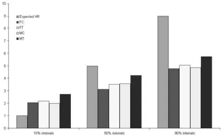
A surprising feature is that, when asked to evaluate how many correct answers belong to their intervals, the average answers are respectively at the 10%, 50% and 90% levels: 3.47, 5.56 and 8.04 for the control group; subjects exhibit overconﬁdence for the calibration task, thinking that they were more cautious than they actually were (see Figure 1). Let us, nevertheless, observe that subjects do predict that their calibration is far from being perfect, otherwise their evaluations would have been 1, 5 and 9.

Figure 1. Expected, Actual and Estimated Hit Rates in the Control Group

These results indicate that not only are people unable to adjust the width of their intervals to the risk level indicated (they are miscalibrated) but they are also unable to predict their bias correctly (they are over or underconﬁ-dent).

To sum up, people seem to overestimate their underconﬁdence and underes-timate their overconﬁdence.

(12)

3.2 The effect of training on miscalibration and

confi-dence in calibration

3.2.1 The general picture

The main purpose of this paper was to see whether a training period during which several incentives aiming at improving people’s calibration as well as decreasing overconﬁdence were provided would be eﬃcient.

Trained subjects have only slightly higher hit rates at the 10%, 50% and 90% level than subjects from the control group (see figure 2). The differences in hit rates between the control and the trained group are not significantly different at any reasonable level. 4

Figure 2. Hit Rates: Control vs Trained Group

We ﬁnd that the median 10% interval width is larger for the trained group than for the control group for 7 questions out of ten. For the 3 remaining

4

The hit rates are respectively at the 10%, 50% and 90% levels 2.03, 3.32 and 4.81 for the control group and 2.40, 3.80 and 5.33 for the trained group.

(13)

questions, the median width of intervals is equal across treatments. Note that this goes in the sense of a worsening of the underconfident miscalibration observed at 10% as people tend to provide too wide intervals at 10%. One reason why we may find such a result is that subjects may not consider the underconfident miscalibration as a bias and consequently, they may not try to correct it.

The same result is found when we compare median widths of 50% in-tervals (wider inin-tervals in the trained group than in the control group for 7 questions, the reverse for 1 question and equal median intervals across treat-ments for the 2 remaining questions). As for 90% intervals, for six questions out of ten the interval width is larger for the trained group while the control group provided wider intervals than the trained group for 1 question. 5

We report the regressions of the interval width of the 10%, 50% and 90% intervals on the sex of the subject, a treatment dummy (=1 if the subject was in the trained group), the interaction between sex and treatment, the age of the subject, his level of education, dummies for the different questions and the interactions between each question and the treatment (see Table 1). We only find the interaction terms between questions 9 and 10 and the treat-ment to be significant and positive in explaining the 50% and 90% interval widths and only the interaction between question 9 and the treatment for the 10% interval width. The treatment makes subjects provide wider 50% and 90% intervals for the last two questions only and it only has a significant and positive effect for the 10% interval width of the 9th question. Note that the level of education has a positive and significant impact on the 10% inter-val width, meaning that more educated subjects tend to provide wider 10% intervals and, by doing so, make their underconfident miscalibration worse. We ran logistic regressions of the dummies "the 10% interval contains the

5

If we compare average interval widths, which seems less relevant as averages are sen-sitive to extreme values, we find that for 7 (6) questions out of ten the average width of 10% and 50% (respectively 90%) intervals are larger for the trained subjects, while for the remaining 3 (respectively 4) questions, the opposite is true.

Checking for the significance of these results with a T-test, we find significantly larger intervals for the trained group than for the control group only for the ninth question, all other differences being not significant. However, as variances of interval widths are often very different across the control and trained group and as a way of eliminating the influ-ence of extreme values, we ran a Wilcoxon-Mann-Whitney test. We found that the 90% interval widths are significantly different (either at the 1%, 5% or 10% levels) for 5 ques-tions out of ten while 10% and 50% intervals widths are significantly different respectively for 3 and 6 questions out of ten.

(14)

correct answer" (ICA10), "the 50% interval contains the correct answer" (ICA50), "the 90% interval contains the correct answer" (ICA90) on the same variables (see Table 2). We observe that the treatment significantly increases the probability for the correct answer to fall in the 50% and 90% intervals provided for almost all of the questions (the interaction terms be-tween the questions and the treatment are always positive and almost always significant). It is true but to a smaller extent for the 10% intervals. If any-thing, our treatment seems to make subjects provide wider intervals (even if this result is far from always reaching significance) and it significantly helps subjects catch the correct answer in their confidence intervals more of-ten. Consequently, the incentives we provided during a short training period decrease the overconfident miscalibration we observe for the 50% and 90% intervals but, to a smaller extent, makes the underconfident miscalibration noticed for the 10% intervals worse.

(15)

Table 1. Regression of the Interval Width of the 10, 50 and 90% intervals

Variable IW10 IW50 IW90 Variable IW10 IW50 IW90 Intercept 125.84063 416.64290 974.49453 q8 -10.39409 -2.99125 0.27977 (0.8355) (0.6064) (0.4887) (0.9850) (0.9968) (0.9998) Sexe -221.24101 -104.93675 -142.78895 q9 1263.63443 2579.99145 4656.41259 (0.3532) (0.7413) (0.7963) (0.0234) (0.0005) (0.0003) Treatment 1.07455 117.31259 38.72279 q10 2578.44365 3218.39626 5653.13829 (0.9984) (0.8682) (0.9749) (<.0001) (<.0001) (<.0001) Sextreatment -39.47164 -301.76110 -79.12153 q2t 25.67114 14.36466 -8.85863 (0.8976) (0.4608) (0.9115) (0.9706) (0.9877) (0.9956) Age -16.75927 -26.84761 -52.72680 q3t 19.30381 20.47461 9.87337 (0.4453) (0.3595) (0.3011) (0.9778) (0.9824) (0.9951) Education 124.22768 86.61469 103.67302 q4t 22.85979 11.05745 -0.38585 (0.0437) (0.2915) (0.4680) (0.9735) (0.9904) (0.9998) q2 -14.99427 -6.77144 3.75704 q5t 26.64393 27.93839 9.36834 (0.9787) (0.9928) (0.9977) (0.9692) (0.9758) (0.9953) q3 0.97352 5.56138 23.04869 q6t 166.74804 385.80898 378.93786 (0.9986) (0.9941) (0.9859) (0.8089) (0.6750) (0.8129) q4 -12.27096 -4.65000 -1.22460 q7t 21.55222 7.43665 -7.34203 (0.9823) (0.9950) (0.9992) (0.9753) (0.9936) (0.9964) q5 21.94779 65.72500 144.65040 q8t 9.55972 -0.79798 -7.32431 (0.9683) (0.9290) (0.9102) (0.9890) (0.9993) (0.9964) q6 214.38529 424.72500 795.61915 q9t 1491.34561 2079.03348 3883.31485 (0.6980) (0.5646) (0.5352) (0.0315) (0.0247) (0.0159) q7 -15.84730 -15.23552 -16.28074 q10t 365.86894 3434.60974 6956.96248 13

(16)

Table 2. Logistic Regression of "the 10, 50, 90% interval contains the correct answer" (ICA10 ICA50 ICA90)

Variable ICA10 ICA50 ICA90 Variable ICA10 ICA50 ICA90 Intercept -0.7402 0.4416 1.3924 q8 -1.1865 -1.8656 -1.4668 (0.2799) (0.4948) (0.0392) (0.0656) (0.0019) (0.0171) Sexe 0.0412 0.3924 0.0738 q9 -1.7349 -2.3641 -2.3985 (0.8915) (0.1391) (0.7711) (0.0190) (0.0002) (0.0002) treatment -0.5951 -1.5940 -1.1804 q10 -1.7381 -1.9947 -1.9420 (0.2896) (0.0048) (0.0485) (0.0188) (0.0011) (0.0020) sextreatment 0.1398 -0.0941 0.2821 q2t 0.8536 1.7735 0.0282 (0.7124) (0.7764) (0.3801) (0.2290) (0.0152) (0.9776) Age 0.00302 0.00324 -0.00832 q3t 0.8063 2.5884 1.5503 (0.9108) (0.8895) (0.7117) (0.3400) (0.0018) (0.0441) Education 0.0507 0.0773 0.0350 q4t 0.7633 2.1252 1.5607 (0.4971) (0.2327) (0.5801) (0.2941) (0.0032) (0.0345) q2 0.2337 -0.3636 1.2972 q5t 0.7561 2.3399 1.6269 (0.6766) (0.5381) (0.1441) (0.4115) (0.0014) (0.0279) q3 -1.3719 -2.8147 -2.3541 q6t -0.7081 1.2329 0.6230 (0.0447) (<.0001) (0.0003) (0.4120) (0.1041) (0.3992) q4 -0.4377 -1.5713 -1.3416 q7t 1.3228 2.1902 1.2944 (0.4481) (0.0074) (0.0291) (0.0935) (0.0034) (0.0833) q5 -1.7691 -1.8656 -1.4668 q8t 1.0284 2.2127 1.5161 (0.0167) (0.0019) (0.0171) (0.1977) (0.0026) (0.0404) q6 -0.7728 -1.8656 -1.3416 q9t 1.0319 2.3218 2.5139 (0.1985) (0.0019) (0.0291) (0.2509) (0.0027) (0.0010) q7 -1.1124 -1.9534 -1.7502 q10t 1.5328 2.3593 1.6794 (0.0856) (0.0015) (0.0052) (0.0804) (0.0015) (0.0246)

Note: _{p-values are in brackets.}

3.2.2 A different impact between genders

This general picture masks some strong heterogeneity across subjects. We can control for several sources of heterogeneity. However, the gender vari-able captures almost all of it. We observe indeed that there is virtually no improvement in women’s calibration especially when we compare the median hit rates between the treatments while men increase their median hit rate

(17)

by 0.5 point at the 50% level and by 1 point at the 10% and 90% levels (see Figure 3).

Figure 3. Hit Rates: Gender Differences

The difference in interval width between the control and the training treatments seems to be larger for men than for women, indicating that men learned more than women to reduce their overconfidence.Using a Wilcoxon-Mann-Whitney test, we find that 10% confidence intervals are significantly wider for the trained group respectively for five questions out of ten and zero question out of ten for men and women. Let us notice that in the trained group both men and women had more than one correct answer inside their 10% intervals exhibiting underconfident miscalibration. As a result, an increase of 10% intervals causes an aggravation of underconfidence. For 50% intervals, the width increases significantly between the control and the training treatments respectively for two and six questions out of ten. Finally, concerning 90% intervals, the difference is significant in three cases and four cases out of ten respectively for women and men.

(18)

3.3 What happened during the training session ?

The training period had an impact on men but almost no eﬀect on women. It could be interesting to use the results from the training period to get an insight into the nature of the learning process that arose. In order to be able to measure learning during the training period, the order of the 20 questions was reversed for half of the subjects.

It appears that during the training process, some learning took place. We measured learning at this stage by comparing the width of the intervals pro-vided for the same question by subjects from the two groups corresponding to the two orders of appearance of the questions. We found that there was a signiﬁcant diﬀerence in the width of the intervals between the two groups for seven questions out of twenty, each going in the sense of longer intervals for the group who answered the question later in the training session. For exam-ple, the intervals provided for question 18 were wider for the group who had the regular order of questions than for those who had the reversed order (for whom question 18 was actually the third one they had to answer). It seems noteworthy that six out of the seven questions which subjects with more training answered with wider intervals were economic knowledge questions.

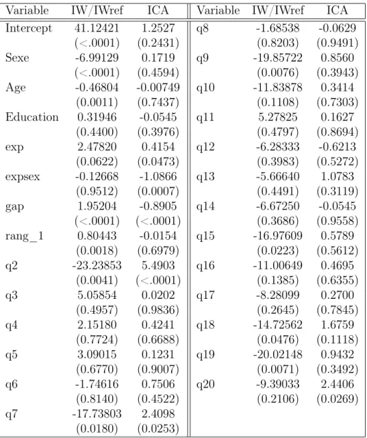
We regressed a variable equal to the interval width chosen over the inter-val width of the interinter-val of reference on the intercept, a dummy indicating the gender ("sex"),the age, the level of education, a dummy indicating whether the question appeared early during the training session ("exp"), the inter-action between "exp" and "sex" ("expsex"), the ranking announced to the subject after he had answered the previous question ("Rank-1"),the gap be-tween the midpoint of the interval provided and the correct answer as a proxy for the ignorance ("gap") and dummies for the different questions (See Table 3). We added "gap" in the regressors so as to take in the effect of knowl-edge on the choice of the interval width. Any residual effect of "Rank-1" can therefore be attributed to competition, ie the effect of the announced rank on the decision to take more or less risk.

Women are found to provide significantly (p-value<0.0001) narrower in-tervals than men. "Age" is also highly significant and negative. "Exp" is pos-itive and significant (p-value=0.0622) indicating that subjects who answered a question later in the training period tend to provide wider intervals. We found that the coefficient of "gap" is positive and highly significant showing that the less people knew the answer, the wider the interval they provided. The coefficient of "Rank-1" was found to be positive and highly significant

(19)

Table 3. Regression of IW/IWref and ICA)

Variable IW/IWref ICA Variable IW/IWref ICA Intercept 41.12421 1.2527 q8 -1.68538 -0.0629 (<.0001) (0.2431) (0.8203) (0.9491) Sexe -6.99129 0.1719 q9 -19.85722 0.8560 (<.0001) (0.4594) (0.0076) (0.3943) Age -0.46804 -0.00749 q10 -11.83878 0.3414 (0.0011) (0.7437) (0.1108) (0.7303) Education 0.31946 -0.0545 q11 5.27825 0.1627 (0.4400) (0.3976) (0.4797) (0.8694) exp 2.47820 0.4154 q12 -6.28333 -0.6213 (0.0622) (0.0473) (0.3983) (0.5272) expsex -0.12668 -1.0866 q13 -5.66640 1.0783 (0.9512) (0.0007) (0.4491) (0.3119) gap 1.95204 -0.8905 q14 -6.67250 -0.0545 (<.0001) (<.0001) (0.3686) (0.9558) rang_1 0.80443 -0.0154 q15 -16.97609 0.5789 (0.0018) (0.6979) (0.0223) (0.5612) q2 -23.23853 5.4903 q16 -11.00649 0.4695 (0.0041) (<.0001) (0.1385) (0.6355) q3 5.05854 0.0202 q17 -8.28099 0.2700 (0.4957) (0.9836) (0.2645) (0.7845) q4 2.15180 0.4241 q18 -14.72562 1.6759 (0.7724) (0.6688) (0.0476) (0.1118) q5 3.09015 0.1231 q19 -20.02148 0.9432 (0.6770) (0.9007) (0.0071) (0.3492) q6 -1.74616 0.7506 q20 -9.39033 2.4406 (0.8140) (0.4522) (0.2106) (0.0269) q7 -17.73803 2.4098 (0.0180) (0.0253)

Note: _{p-values are in brackets.}

too. It seems that the announcement of a bad ranking leads subjects to take less risk and provide wider intervals.

The logistic regression of the probability to catch the correct answer in one’s interval (ICA) on the same variables (See Table 3) reveals that while

(20)

"sex" "age" and "rank-1" are not significant, "gap" is negative and highly significant showing that the more ignorant the subject was about the answer, the less chance for the correct answer to belong to his interval. "exp" is found to be positive (p-value=0.0473) and "expsex" negative (p-value=0.0007) in-dicating that, overall, having answered a greater number of questions pre-viously tends to increase one’s chances to catch the correct answer in his interval but the opposite is actually true for men. We tried to search for explanations for the fact that women failed to learn from our training period while men did. It seems likely that the explanation lies in what happens in the training period. The different possible explanations are: a stronger reaction to competition for men than for women, a longer time for decision, the fact that money is a stronger incentive for men... Unfortunately, the too scarce data available to us made it impossible to reach a definitive conclu-sion. Our results could indicate that men used more the training session to experiment different strategies and took more risk to go up in the ranking and, as a result, benefited more from the training period than women who were more cautious. This is in line with the idea of Gail Osten, author of "What Can Male Traders Learn from Successful Women...And Vice Versa" who says that "women, particularly when starting out, often are more timid in trading and more conservative in the use of their money". ŞMen, on the other hand, seem not to have the same reservation or feeling of guilt regard-ing their initial fundregard-ing or the price of tuition,Ť accordregard-ing to Barb Magio, a trader, educator and moderator in woodiescciclub.com. ŞThey take these losses merely as part of the learning process and seem to feel less guilt or necessity to explain why instant profitability is lacking.Ť

To conclude, providing monetary incentives helps reduce men’s overcon-ﬁdent miscalibration but leaves women’s miscalibration unchanged.

4 Discussion

This paper contributes to a literature interested in cognitive biases having economic consequences. We focus on miscalibration, a very robust bias corre-lated with losses on experimental financial markets and bad entrepreneurship. In line with the existing literature on miscalibration, our subjects strongly suffer from the miscalibration bias, their 50% and 90% intervals being too narrow (overconfident miscalibration). We find that subject’s 10% intervals are too wide (underconfident miscalibration). These results are widespread in

(21)

the population according to the literature and there are very few exceptions. Furthermore, subjects overestimate their underconfidence and underestimate their overconfidence. The fact that people overestimate their underconfident miscalibration could mean that they do not consider it as a bias. Maybe being too cautious is seen as a good thing. Previous attempts to reduce miscalibration relied on very long and repetitive training periods.

We find that men’s calibration can be improved by a thirty-minute train-ing period punishtrain-ing miscalibrated behavior by money losses, while women’s cannot. The incentives we implemented had no effect on women. This differ-ence in the impact of monetary incentives between genders is a key interest of Niederle and her coauthors (?Niederle and Vesterlund, 2007, Niederle and Yestrumskas, 2007) who show that it can be detrimental to welfare. Indeed, they highlight the fact that highly able women do not enter tournaments as often as they should while low performing men enter too often. To overcome this issue, Niederle et al. (2007)studied the effect of affirmative action in fa-vor of women and found that it increased the number of women willing to enter the tournament and decreased the number of men, more than what would be predicted solely by the change in the probability of winning. There are probably other incentives one could think of that would have a stronger effect on women than on men and which could therefore benefit welfare.

5 Conclusion

We find that people who went through the training session provide wider intervals at 10, 50 and 90% than those who did not. This result is not always significant but it is quite robust as subjects from the control group never provided significantly wider intervals than trained subjects. Moreover, our training significantly increases a subject’s chance to catch the correct answer in his interval. This results in an improvement of calibration at the 50% and 90% levels but the underconfident miscalibration observed at the 10% level is made worse by the training. Nevertheless, men seem to have learned more from the training than women, as the increase in interval width between the treatments is greater for men than for women in most cases. As a result, the difference in hit rates between the control and the trained group is greater for men, who become more cautious and increase their hit rates at the three levels while women’s hit rates are virtually the same across treatments.

(22)

disap-pears in a market environment, since we provided the kind of incentives that are expected on real markets. According to our results, real traders are likely to underestimate the risk they take when they think they invested in a very secure asset. Symmetrically they take less risks than they think when they invest in risky assets. So, the overall eﬀect of miscalibration on real markets is ambiguous. Our results also suggest that men may be more successful in learning calibration. Women traders may need a longer king of training which would give them more time to get rid of their overcautiousness.

(23)

Author’s Affiliations

Marie-Pierre Dargnies(Corresponding author) Université Paris 1 Panthéon-Sorbonne,

Paris School of Economics

Address: Centre d’Economie de la Sorbonne,

106-112 Boulevard de l’Hôpital 75013 Paris, France. Tel:(0033) 1 44 07 82 13.

Fax: (0033) 1 44 07 82 31.

E-mail: marie-pierre.dargnies@univ-paris1.fr and

Guillaume Hollard Paris School of Economics, CNRS.

(24)

Acknowledgements

We are very grateful to Michèle Cohen, Jordi Brandts, Denis Hilton, Bob Slonim, Jean-Christophe Vergnaud, Jean-Robert Tyran, James Andreoni, Pedro Dal Bo, Maxim Frolov, Gilles Bailly, Natacha Raﬃn, Victor Hiller and Thomas Baudin. We are grateful to numerous seminar participants at the JEE conference in Lyon, especially Glenn Harrison, and at the University of Paris 1 and Brown University.

(25)

Appendices

A

Instructions

A.1 Trained group

You are about to participate to an experiment aiming at evaluating your ability to calibrate risk. This experiment will be divided in several steps.

A.1.1 First step

In this ﬁrst step, you will have to answer a set of twenty questions by providing an interval for each question. At the beginning of this step, you will be endowed with 2000 points which will be converted to euros at the end of the experiment. For each of the 20 questions, 100 points will be at stake. You will have to keep the more points you can.

For each question, you will be provided with an interval of reference including the correct answer. The interval you will provide will have to be contained in the interval of reference. Your payoﬀs will be determined as follows:

• If the correct answer does not belong to the interval chosen, you will lose the 100 points at stake for the question. They will be withdrawn from your endowment.

• If the correct answer does belong to the interval chosen, the narrower the interval you chose, the more points you will keep. Your payoﬀs will depend on the diﬀerence between the length of the interval chosen and the length of the interval of reference given the following formula:

payment =         

−100 ∗ _{width of the interval of reference}width of the interval provided if the correct answer belongs to the interval provided

−100 otherwise

In consequence, the wider the interval chosen, the more chances for the cor-rect answer to belong to your interval but the fewer the points you will get to keep if your interval contains the correct answer.

(26)

Symmetrically, the narrower the interval chosen, the less chances for the correct answer to belong to your interval but the more points you will get to keep if your interval contains the correct answer.

After each question, you will see the correct answer, the intervals chosen for the same question by the subjects present in the lab (ranked from the narrower to the wider) as well as the number of points they kept.

Example: For the question, "How old was John Fitzgerald Kennedy when he died?", if the interval of reference is [30;80]:

• If you give the interval [49;54], your potential loss is 10: if the correct answer belongs to the interval [49;54], you will keep 90 points out of the 100 points at stake for this question. Here, your actual loss would be 100 points as the correct answer, 46, does not belong to your interval. Hence, you would have lost the 100 points at stake for this question. • If you give the interval [40;65], your potential loss is 50 and it

corre-sponds to your actual loss as the correct answer belongs to your interval. In this case, you would have kept 50 points out of the 100 points at stake for this question.

A.1.2 Second step

In this second step, you will also be compensated but you will only be in-formed of the details of the remuneration afterwards. You will have to answer to a set of 10 questions by providing your best estimate of the answer and conﬁdence intervals, ie a lower and an upper bound corresponding to a cer-tain level of conﬁdence that the correct answer falls between these 2 values, knowing that:

• The narrower the interval you will provide, the more chances for the correct answer to fall outside.

• The wider the interval you will provide, the more chances for the correct answer to fall inside.

For each question, you will have to give intervals corresponding to 3 different levels of confidence (10%, 50% and 90%). To help you calibrate the risk, here are 3 different and equivalent ways to understand what a 10% interval is: A 10% interval corresponds to a lower and an upper values such that:

(27)

1. You are 10% conﬁdent that the correct answer lies between these 2 values.

2. For 10 questions, 1 correct answer on average belongs to the interval provided and 9 correct answers out of 10 on average fall outside of their interval.

3. You think there are 9 chances out of 10 for the correct answer to fall outside your interval.

Example of question: What was the year of Vincent Auriol’s election as President?

If you give the value 1927 as your best estimation of the answer and the intervals [1921,1930] at 10%, [1915,1935] at 50% and [1915,1949] at 90%, it means that:

• Your best estimate of the year Vincent Auriol was elected is 1927. • You are 10% conﬁdent he was elected between 1921 and 1930.

• You think there is 1 chance out of 2 that he was elected before 1915 or after 1935.

(28)

Considering the 10 questions you just answered, please evaluate:

• The number of correct answers falling inside the 10% intervals you provided (please enter a number between 0 and 10).

As well as:

• The number of correct answers falling inside the 10% intervals provided by the average subject (please enter a number between 0 and 10). • The number of correct answers falling inside the 50% intervals provided

by the average subject (please enter a number between 0 and 10). • The number of correct answers falling inside the 90% intervals provided

by the average subject (please enter a number between 0 and 10). For each correct evaluation, you will earn 100 points.

Finally, you will have to make 2 choices each time between 2 bets. For each of these 2 choices, you will earn 300 points if what you bet on happens.

A.2 Control group

You are about to participate to an experiment aiming at evaluating your ability to calibrate risk.

You will be compensated but you will only be informed of the details of the remuneration afterwards. You will have to answer to a set of 10 questions by providing your best estimate of the answer and conﬁdence intervals, ie a lower and an upper bound corresponding to a certain level of conﬁdence that the correct answer falls between these 2 values, knowing that:

• The narrower the interval you will provide, the more chances for the correct answer to fall outside.

• The wider the interval you will provide, the more chances for the correct answer to fall inside.

(29)

References

Adams, P. and J. Adams (1958). The effects of feedback on judgmental interval predictions. American Journal of Psychology 71, 747–751.
Biais, B., D. Hilton, K. Mazurier, and S. Pouget (2005). Judgmental over-confidence, self-monitoring and trading performance in an experimental financial market. Review of Economic Studies 72, 287–312.
Bonnefon, J., D. Hilton, and D. Molian (2005). A portrait of the unsuccessful entrepreneur as a miscalibrated thinker. Working Paper.
Cesarini, D., O. Sandewall, and M. Johannesson (2006). Confidence interval estimation tasks and the economics of overconfidence. Journal of Economic Behavior and Organization 61, 453–470.
Glaser, M., T. Langer, and M. Weber (2005). Overconfidence of professionals and laymen: Individual differences within and between tasks?
Klayman, J., J. Soll, and S. Barlas (1999). Overconfidence: It depends on how, what, and whom you ask. Organizational Behavior and Human Decision Processes 79(3), 216–247.
Lichtenstein, S. and P. Fischhhoff (1977). Do those who know more also know more about what they know? Organizational Behavior And Human Performance 20, 159–183.
Lichtenstein, S. and B. Fischhoff (1980). Training for calibration. Organiza-tional Behavior And Human Performance 26, 149–171.
Niederle, M., C. Segal, and L. Vesterlund (2007). How costly is diversity? affirmative action in competitive environments. Working Paper.
Niederle, M. and L. Vesterlund (2007). Do women shy away from competi-tion? do men compete too much? Quarterly Journal of Economics 122, 1067–1101.
Niederle, M. and A. Yestrumskas (2007). Gender differences in seeking chal-lenges: The role of institutions. Working Paper.
Pickhardt, R. and J. Wallace (1974). A study of the performace of subjective probability assessors. Decision Sciences 5, 347–363.
Regner, I., D. Hilton, L. Cabantous, and S. Vautier (2006). Judgmental overconfidence:cognitive bias or positive illusion? Working Paper.