The Dynamics of State Policy Liberalism, 1936-2014
The MIT Faculty has made this article openly available. Please share
how this access benefits you. Your story matters.
Citation Caughey, Devin, and Christopher Warshaw. “The Dynamics of State
Policy Liberalism, 1936-2014: THE DYNAMICS OF STATE POLICY LIBERALISM.” American Journal of Political Science 60.4 (2016): 899–913.
As Published http://dx.doi.org/10.1111/ajps.12219
Publisher Wiley Blackwell
Version Author's final manuscript
Citable link http://hdl.handle.net/1721.1/105870
Terms of Use Creative Commons Attribution-Noncommercial-Share Alike
The Dynamics of State Policy Liberalism, 1936–2014
Devin Caughey
∗Department of Political Science
MIT
Christopher Warshaw
†Department of Political Science
MIT
First draft: March 5, 2014 This draft: March 4, 2015
Abstract
Applying a dynamic latent-variable model to data on 148 policies collected over eight decades (1936–2012), we produce the first yearly measure of the policy liberalism of U.S. states. Our dynamic measure of state policy liberalism marks an important advance over existing measures, almost all of which are purely cross-sectional and thus cannot be used to study policy change. We find that, in the aggregate, the policy liberalism of U.S. states steadily increased between the 1930s and 1970s and then largely plateaued. The policy liberalism of most states has remained stable in relative terms, though several states have shifted considerably over time. We also find surprisingly little evidence of multidimensionality in state policy outputs. Our new estimates of state policy liberalism have broad application to the study of political development, representation, accountability, and other important issues in political science.
We appreciate the excellent research assistance of Melissa Meek, Kelly Alexander, Aneesh Anand, Ti↵any Chung, Emma Frank, Jose↵ Kolman, Mathew Peterson, Steve Powell, Charlotte Swasey, Lauren Ullmann, and Amy Wickett. We also appreciate the willingness of Frederick Boehmke and Carl Klarner to generously share their data. We are grateful for research support from the Dean of the School of Humanities, Arts, and Social Sciences at MIT. All mistakes, however, are our own.
∗Assistant Professor, Department of Political Science, Massachusetts Institute of Technology,
caughey@mit.edu
†Assistant Professor, Department of Political Science, Massachusetts Institute of Technology,
“Change,” Chandler et al. (1974, 108) noted four decades ago, “is both methodologically and substantively critical for any theory of policy.” This is true of both of the determinants of government policies, such as shifts in public mood or changes in the eligible electorate (e.g., Stimson, MacKuen, and Erikson 1995; Husted and Kenny 1997), and of policy feedback on political and social outcomes (e.g., Wlezien 1995; Campbell 2012). Theories of all these phenomena rely explicitly or implicitly on models of policy change. Moreover, many of the most ambitious theories focus not on individual policies or policy domains, but on the character of government policy as a whole. In short, most theories of policymaking are both dynamic and holistic: they are concerned with changes in the general orientation of government policy.
Unfortunately, the literature on U.S. state politics, perhaps the most vibrant field for testing theories of policymaking, relies almost exclusively on policy indicators that are either measured at a single point in time (e.g., Wright, Erikson, and McIver 1987) or else cover only a partial subset of state policy outputs (e.g., Besley and Case 2003).1 Static measures
are poorly suited to studying causes of policy change over time (Lowery, Gray, and Hager 1989; Ringquist and Garand 1999; Jacoby and Schneider 2009). And while domain-specific measures may provide useful summaries of some aspects of state policy, such as welfare spending (Moffitt 2002) or gay rights (Lax and Phillips 2009a), they are at best imperfect proxies for what is often the outcome of interest, the overall orientation of state policy.
In this paper, we develop a holistic yearly summary of the ideological orientation of state policies, which we refer to as state policy liberalism. This measure is based on a unique dataset of 148 policies, which covers nearly eight decades (1936–2014) and includes policy domains ranging from labor regulation and civil rights to gun control and gay rights.2 Based
on these data, we estimate policy liberalism in each year using a dynamic Bayesian
latent-1. To our knowledge, the only existing holistic yearly summary of state policies is Jacoby and Schneider’s (2009) measure of particularistic versus collective state spending priorities between 1982 and 2005. As we discuss below, our measures di↵er substantially in time coverage, conceptual interpretation, and the data used to construct them.
2. Both the policy data and our policy liberalism estimates will be made available to the public upon publication of this article.
variable model designed for a mix of continuous, ordinal, and dichotomous policy indicators. This measurement model enables us to make use of many indicators of policy liberalism, thus substantially reducing measurement error on the estimates of our construct of interest. Despite the disparate policy domains covered by our dataset, allowing for additional latent policy dimensions does little to improve the predictive accuracy of the model. This suggests that contrary to previous claims (e.g., Sorens, Muedini, and Ruger 2008), a single latent dimension suffices to capture the systematic variation in state policies. Consistent with this conclusion, our dynamic measure is highly correlated with existing cross-sectional measures of state policy liberalism as well as with issue-specific ideological scales.
Substantively, we find that while U.S. states as a whole have drifted to the left (that is, they have increasingly adopted liberal policies), most have remained ideologically sta-ble in relative terms. Across our entire time series, the most conservative states are in the South, whereas California, New York, Massachusetts, and New Jersey are always among the most liberal. The relative policy liberalism of a few states, however, has changed substan-tially. Several Midwestern and Mountain states have become considerably more conservative relative to the rest of the nation, whereas most of the Northeast has become more liberal.
Our new dynamic estimates can be used to study a wide variety of possible questions, many of which are not easily investigated using cross-sectional measures. Potential topics of study include the short- and long-term determinants of policy outputs, such as economic development, political institutions, mass policy preferences, and electoral outcomes. Policy liberalism could also be used as an independent variable, as a means of examining policy feedback or other consequences of policy change. These measures thus o↵er new research av-enues onto political development, representation, accountability, and other important issues in political science.
The remainder of the paper is organized as follows. We begin by defining the concept of policy liberalism and situating it in the literature on U.S. state politics and policy. Next, we describe our policy dataset, our measurement model, and our yearly estimates of state policy
liberalism. We then provide evidence for the validity of our measure. We show that it is highly correlated with existing measures of policy liberalism and related concepts, and that a one-dimensional scale adequately accounts for systematic policy variation across states. The penultimate section discusses potential applications of our measure, illustrating its usefulness with an analysis of the policy e↵ects of voter registration laws. The final section concludes.
Measuring State Policies
Studies of state policy generally employ one of two measurement strategies: they either con-sider policy separately using policy-specific indicators, or they construct composite measures intended to summarize the general orientation of state policies within or across domains (Jacoby and Schneider 2014, 568). Among studies in the first camp, some have focused on whether or not states have particular policies. Lax and Phillips (2009a), for example, exam-ine the representational congruence between a series of dichotomous state gay-rights policies and state opinion majorities. Other studies have employed continuous policy-specific indi-cators, such as welfare expenditures (Husted and Kenny 1997), tax rates (Besley and Case 2003), or minimum wages (Leigh 2008), which potentially have greater sensitivity to dif-ferences between states. Whether dichotomous or continuous, policy-specific measures are appropriate when the research question is limited to a particular policy area. But they are suboptimal as summary measures of the general orientation of state policies, though this is how they are often used.3
For this reason, a number of scholars have sought to combine information from multiple policies, using factor analysis or other dimension-reduction methods to summarize them in terms of one or more dimensions of variation. Dimension reduction has several advantages over policy-specific measures. First, from a statistical point of view, using multiple
indica-3. Lax and Phillips (2009a, 369) claim that “using. . . policy-specific estimates” allows them to “avoid problems of inference that arise when policy and opinion lack a common metric.” On a policy-by-policy basis this is probably true. But evaluating congruence on state policy in general, or even just in the domain of gay rights, requires that the policy-specific estimates of congruence be weighted or otherwise mapped onto a single dimension. Thus, dimension reduction must occur at some point, whether at the measurement stage or later in the analysis.
tors for a latent trait usually reduces measurement error on the construct of interest, often substantially (Ho↵erbert 1966; Ansolabehere, Rodden, and Snyder 2008). Secondly, many concepts require multiple indicators to adequately represent the full content or empirical do-main of the concept. For example, the concept of liberalism, in its contemporary American meaning, encompasses policy domains ranging from social welfare to environmental protec-tion to civil rights. A measure of liberalism based on only a subset of these domains would thus fare poorly in terms of content validation (Adcock and Collier 2001, 538–40). A final benefit is parsimony. If a single measure can predict variation in disparate domains, then we have achieved an important desideratum of social science: “explaining as much as possible with as little as possible” (King, Keohane, and Verba 1994, 29).
Di↵erent works have identified di↵erent traits or dimensions underlying state policies. Walker (1969), for example, creates an “innovation score” that captures the speed with which states adopt new programs. Sharkansky and Ho↵erbert (1969) identify two latent factors that structure variation in state policies, as do Sorens, Muedini, and Ruger (2008). Hopkins and Weber (1976) uncover a total of five. But primarily the state politics literature has focused on a single left–right policy dimension (e.g., Ho↵erbert 1966; Klingman and Lammers 1984; Wright, Erikson, and McIver 1987; Gray et al. 2004). As a number of studies have confirmed, states with minimal restrictions on abortion tend to ban the death penalty, regulate guns more tightly, o↵er generous welfare benefits, and have progressive tax systems, and vice versa for states with more restrictive abortion laws. Following Wright, Erikson, and McIver (1987), we label this dimension policy liberalism.
What is policy liberalism? We conceptualize liberalism not as a logically coherent ideol-ogy, but as a set of ideas and issue positions that, in the context of American politics, “go together” (Converse 1964). Relative to conservatism, liberalism involves greater government regulation and welfare provision to promote equality and protect collective goods, and less government e↵ort to uphold traditional morality and social order at the expense of personal autonomy. Conversely, conservatism places greater emphasis on the values of economic
free-dom and cultural traditionalism (e.g., Ellis and Stimson 2012, 3–6). Although the definitions of liberalism and conservatism have evolved over time, with civil rights and then social issues becoming more salient relative to economics (Ladd 1976, 589–93), these ideological cleavages have existed in identifiable form since at least the mid-20th century (Schickler 2013; Noel 2014).
There are several things to note about this definition of policy liberalism. First, it is comprehensive, in that it covers most if not all domains of salient policy conflict in American domestic politics.4 This is not to say that policy liberalism explains all variation in state policy, or that all policies are equally structured by this latent dimension. But it is a concept that attempts to summarize, holistically, all the policy outputs of a state. Second, we define policy liberalism solely in terms of state policies themselves. By contrast, some previous measures (e.g., Sharkansky and Ho↵erbert 1969; Hopkins and Weber 1976) incorporate so-cietal outcomes like infant mortality rates and high school graduation rates, muddying the distinction between government policies and socio-economic conditions (Sorens, Muedini, and Ruger 2008).
A final characteristic of our conceptualization of policy liberalism, which is particularly crucial for our purposes, is that it is dynamic. Unlike, say, state political culture (Elazar 1966), which changes slowly if at all, policy liberalism can and does vary across time in response to changes in public opinion, partisan control, and social conditions. Defining policy liberalism as a time-varying concept is hardly controversial, but it does conflict with previous operationalizations of this concept, all of which are cross-sectional. Cross-sectional measures are problematic for two reasons. First, many are based on data from a long time span—over a decade, in the case of Wright, Erikson, and McIver (1987)—averaging over possibly large year-to-year changes in state policy (Jacoby and Schneider 2001). More importantly, cross-sectional measures preclude the analysis of policy change, which not only is theoretically limiting, but also inimical to strong causal inference since the temporal order of the variables
4. We do not include foreign policy in the domain of policy liberalism because states typically do not make foreign policy.
cannot be established (Lowery, Gray, and Hager 1989; Ringquist and Garand 1999).
To our knowledge, the only existing time-varying measure that provides a holistic sum-mary of state policy outputs is the measure of policy spending priorities developed by Jacoby and Schneider (2009).5 This measure, available annually between 1982 and 2005, is estimated
with a spatial proximity model using data on the proportions of state budgets allocated to each of nine broad policy domains (corrections, education, welfare, etc.). Jacoby and Schnei-der interpret their measure as capturing the relative priority that states place on collective goods versus particularized benefits, an important concept in the theoretical literature on political economy (e.g., Persson and Tabellini 2006) as well as in empirical work on state politics (e.g., Gamm and Kousser 2010).
Despite both being holistic yearly policy measures, policy liberalism and policy priorities di↵er in important ways. As Jacoby and Schneider emphasize, policy liberalism and policy priorities are conceptually distinct; indices of policy liberalism “simply do not measure the same thing” as their policy priorities scale (2009, 19). For example, the policy priorities scale is not intended to capture “how much states spend” but rather “how states divide up their yearly pools of available resources” (Jacoby and Schneider 2009, 4). Consequently, variation in the size of government, which lies at the heart of most liberal–conservative conflict (e.g., Meltzer and Richard 1981; Stimson 1991), is orthogonal to their measure. Another salient di↵erence is that the policy priorities scale is based solely on state spending data. This endows their measure with a direct and intuitive interpretation, but at the cost of excluding taxes, mandates, prohibitions, and other non-spending policies that shape the lives of citizens in equally important ways. Our policy liberalism measure resolves this trade-o↵ di↵erently, emphasizing broad policy coverage at the possible expense of intuitive interpretation.
In summary, there is no existing time-varying measure of state policy liberalism, one of the central concepts of state politics. Nearly all existing summaries of state policy orientations are cross-sectional. Those that are dynamic either examine policy liberalism in a particular
policy area or, in the case of Jacoby and Schneider’s policy priorities scale, measure a di↵erent concept entirely. Thus what is required is a measurement strategy that summarizes the global ideological orientation of state policies using time-varying data that capture the full empirical domain of policy liberalism.
Policy Data
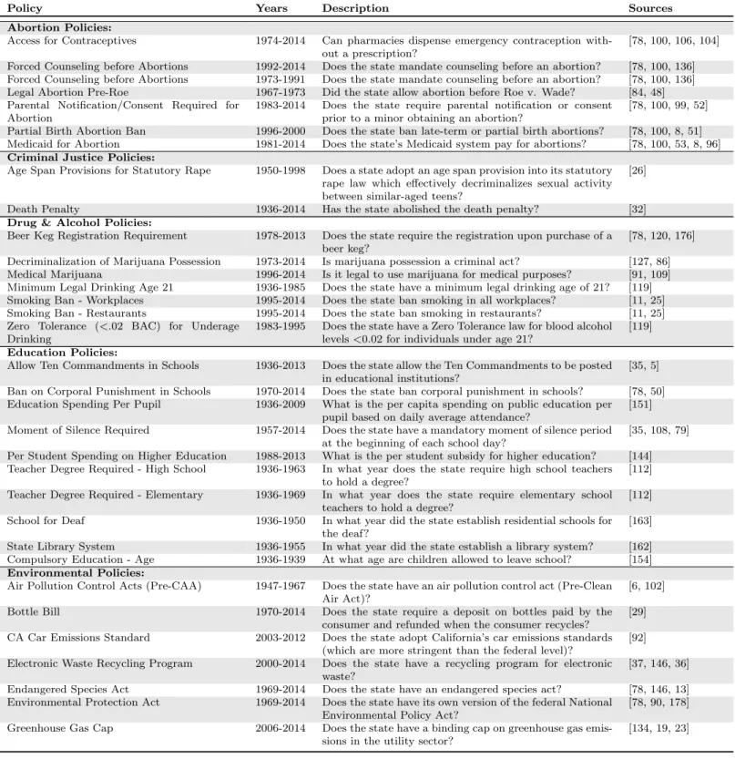
As Jacoby and Schneider (2014) observe, composite measures of policy liberalism risk tau-tology if they are derived from policy indicators selected for their ideological character. Although the resulting scale may be a valid measure of policy liberalism, selection bias in the component indicators undermines any claim that state policies vary along a single di-mension. For this reason, we sought to make our dataset of state policies as comprehensive as possible, so as to allow ideological structure to emerge from the data rather than imposing it a priori. Given resource constraints and data limitations, we cannot claim to have con-structed a random sample of the universe of state policies (if such a thing is even possible). We are confident, however, that our dataset of 148 distinct policies is broadly representative of the policy outputs of states across a wide range of domains. (For complete details on the policies in our dataset, see the online appendix accompanying this article.)
To be included in our dataset, a policy had to meet the following criteria. First, it had to be a policy output rather than a policy outcome (i.e., an aspect of the social environment a↵ected by policy) or a government institution (i.e., one of the basic structures or rules of the government). For example, we excluded state incarceration and infant-mortality rates, which we considered outcomes. We also excluded indicators for whether states had particular legislative rules or government agencies, which we classified as institutions.6 Second, the
policy had to be politically salient. To identify salient policies, we canvassed books and articles on state politics, legal surveys of state policies, state party platforms, governors’ biographies, state-specific political histories, and government and interest-group websites.
6. The dataset used in this paper excludes electoral policies as well. We do this for the pragmatic reason that scholars may want to use our measure to examine the e↵ect of such policies.
Third, the policies had to be comparable across all states. Many environmental, parks, and farm policies, for example, are not comparable across states due to fundamental di↵erences in state geography (e.g., coastal versus non-coastal). Some policies we normalized by an appropriate baseline to make them more comparable.7 Finally, in keeping with our focus
on dynamics, data on a given policy had to be available in comparable form in at least five di↵erent years.
The actual policy data themselves were obtained from many di↵erent sources, including government documents, the Book of the States, interest-group publications, and various secondary sources.8 Over four-fifths of the policies are ordinal (primarily dichotomous), but
the 26 continuous variables provide disproportionate information because they di↵erentiate more finely between states.9 The policy domains covered by the dataset include
• abortion (e.g., parental notification requirements for minors) • criminal justice (e.g., the death penalty)
• drugs and alcohol (e.g., marijuana decriminalization)
• education (e.g., per-pupil education spending; ban on corporal punishment) • the environment (e.g., protections for endangered species)
• civil rights (e.g., fair employment laws; gay marriage) • gun control (e.g., handgun registration)
• labor (e.g., right-to-work laws)
• social welfare (e.g., AFDC/TANF benefits) • taxation (e.g., income tax rates)
and miscellaneous other regulations, such as fireworks bans and bicycle helmet laws.
To validate the comprehensiveness of our dataset, we can compare its coverage to other datasets that were constructed for di↵erent purposes. For example, our policies cover 17
7. We adjusted all monetary expenditure and welfare benefit policies into 2012 dollars. We also adjusted for cost-of-living di↵erences between states (Berry, Fording, and Hanson 2000).
8. In general, we tried to obtain primary sources for each policy indicator. When this proved impossible, we obtained multiple secondary sources to corroborate the information about each policy in our database.
of the 20 non-electoral policy areas contained in Sorens, Muedini, and Ruger’s (2008) state policy database. Similarly, seven of the eight policy categories in the National Survey of State Laws, a lengthy legal compendium of “the most-asked about and controversial” state statutes, are represented in our dataset (Leiter 2008, xii).10 Our data also include 40 of the 56 policy
outputs in Walker’s (1969) policy innovation dataset and 21 of the 34 non-electoral policies examined by Lax and Phillips (2011).11 The overlap between these last three datasets and
ours is particularly significant, because none of the three were constructed for the purpose of studying the ideological structure of state policies. Even Sorens, Muedini, and Ruger (2008), who do analyze policy in ideological terms, conceive of state policies as varying along two dimensions. In sum, our dataset, while not a random sample of the universe of policies, is broadly representative of available data on the salient policy activities of U.S. states.
Measurement Model
We use the policy dataset described above to construct yearly measures of state policy liberalism. Like most previous work on the subject, we treat policy liberalism as a latent variable whose values can be inferred from observed policy indicators. Our latent-variable model (LVM), however, o↵ers several improvements over previous measurement strategies, most of which have relied on factor analysis applied to cross-sectional data. First, we use a Bayesian LVM, which unlike classical factor analysis provides straightforward means of characterizing the uncertainty of the latent scores and also easily handles missing data by imputing estimates on the fly (Jackman 2009, 237–8). Second, most of our policy indicators are dichotomous variables, a poor fit for a factor-analytic model, which assumes that the observed indicators are continuous. We therefore follow Quinn (2004) and specify a mixed LVM that models continuous indicators with a factor-analytic model and ordinal (including
10. The categories are Business and Consumer, Criminal, Education, Employment, Family, General Civil, Real Estate, and Tax. There are no real estate laws in our dataset because we could not locate comparable time-varying data on these laws.
11. The remaining policies are missing either because time-varying data were not available or because the policies are not sufficiently comparable across states.
dichotomous) variables with an item-response model. Third, our measurement model is dynamic, both in that it allows policy liberalism to vary by year and in that it specifies a dynamic linear model that links the measurement model between periods.
We parameterize policy liberalism as a latent trait ✓st that varies across states and years.
For each state s and year t, we observe a mix of J continuous and ordinal policies, denoted yst = (y1st, . . . , yjst, . . . , yJst), whose distribution is governed by a corresponding vector of
latent variables y⇤st. We model y⇤st as a function of policy liberalism (✓st) and item-specific
parameters ↵t = (↵1t, . . . , ↵jt, . . . , ↵Jt) and = ( 1, . . . , j, . . . , J),
y⇤st ⇠ NJ( ✓st ↵t, ), (1)
where NJ indicates a J-dimensional multivariate normal distribution and is a J ⇥ J
covariance matrix. In this application, we assume to be diagonal, but this assumption could be relaxed to allow for correlated measurement error across variables. Note that ↵jt,
which is analogous to the “difficulty” parameter in the language of item-response theory, varies by year t, whereas the “discrimination” j is assumed to be constant across time.
We accommodate data of mixed type via the function linking latent and observed vari-ables. If policy j is continuous, we assume y⇤
jst is directly observed (i.e., yjst = yjst⇤ ), just
as in the conventional factor analysis model. If policy j is ordinal, we treat the observed yjst as a coarsened realization of y⇤jst whose distribution across Kj > 1 ordered categories is
determined by a set of Kj+ 1 thresholds ⌧j = (⌧j0, . . . , ⌧jk, . . . , ⌧j,Kj). Following convention,
we define ⌧j0 ⌘ 1, ⌧j1 ⌘ 0, and ⌧jKj ⌘ 1, and we set the diagonal elements of that
cor-respond to ordinal variables equal to 1. As in a ordered probit model, yjst falls into category
k if and only if ⌧j,k 1 < yjst⇤ ⌧jk. Thus for ordinal variable j, the conditional probability
that y⇤
jst ⇠ N( j✓st ↵jt, 1) is observed as yjst = k is
Pr(⌧j,k 1 < yjst⇤ ⌧jk | j✓st ↵jt) = Pr(yjst⇤ ⌧jk | j✓st ↵jt) Pr(yjst⇤ ⌧j,k 1 | j✓st ↵jt)
where is the standard normal CDF (Fahrmeir and Raach 2007, 329). In the dichotomous case, where there are Kj = 2 categories (“0” and “1”), the conditional probability that yjst
falls in the second category (i.e., “1”) is
Pr(⌧j1< y⇤jst ⌧j2 | j✓st ↵jt] = (⌧j2 [ j✓st ↵jt]) (⌧j1 [ j✓st ↵jt])
= ( j✓st ↵jt), (3)
which is identical to the conventional probit item-response model (Quinn 2004, 341).
We allow the ↵jt to vary by year to account for the fact that many policies (e.g.,
seg-regation laws) trend over time towards universal adoption or non-adoption. The simplest way to deal with this problem is to estimate the difficulty parameters anew in each year. A more general approach, however, which pools information about ↵jt over time, is to model
the evolution of the ↵jt with a dynamic linear model, or DLM (West and Harrison 1997;
Jackman 2009, 471–2). In this application we use a local-level DLM, which models ↵jt using
a “random walk” prior centered on ↵j,t 1:
↵jt ⇠ N(↵j,t 1, ↵2). (4)
If there is no new data for an item in period t, then the transition model in Equation 4 acts as a predictive model, imputing a value for ↵jt (Jackman 2009, 474). The transition variance
2
↵ controls the degree of smoothing over time. Setting ↵2 =1 is equivalent to estimating
↵jt separately each year, and ↵2 = 0 is the same as assuming no change over time. We take
the more agnostic approach of estimating 2
↵ from the data, while also allowing it to di↵er
between continuous and ordinal variables.
The parameters in an LVM cannot be identified without restrictions on the parameter space (e.g., Clinton, Jackman, and Rivers 2004). In the case of a one-dimensional model, the direction, location, and scale of the latent dimension must be fixed a priori. We identify the location and scale of the model by post-processing the latent measure of state policy
liberalism to be standard normal. For the prior on the innovation parameter ↵, we use a
half-Cauchy distribution with a mean of 0 and a scale of 2.5 (Gelman 2006). The difficulty and discrimination parameters are drawn from normal distributions with a mean of 0 and a standard deviation of 10. We fix the direction of the model by constraining the sign of a small number of the item parameters (Bafumi et al. 2005).12 We further constrain the
polarity by assigning an informed prior to the policy measure for four states in year t = 0 (Martin and Quinn 2002).13 We estimated the model using the program Stan, as called
from R (Stan Development Team 2013; R Core Team 2013).14 Running the model for 1,000 iterations (the first 500 used for adaptation) in each of 4 parallel chains proved sufficient to obtain satisfactory samples from the posterior distribution.
Estimates of State Policy Liberalism
Estimating our measurement model using the policy data described earlier produces a mea-sure of the policy liberalism of each state in each year 1936–2014. When interpreting these estimates, one should bear in mind that the model allows the difficulty parameters ↵t to
evolve over time. As a result, aggregate ideological shifts common to all states will be par-tially assigned to the policy difficulties. Since states did adopt increasingly liberal policies over this period, the model partially attributes this trend to the increasing difficulty of con-servative policies (and increasing “easiness” of liberal ones). If we modify the model so as to hold the item difficulties constant over time, the policies of all U.S. states are estimated to
12. Specifically, we constrain continuous measures of state spending to have a positive discrimination pa-rameter, which implies that more liberal states spend more money. We also constrain the polarity of four dichotomous items. The discrimination of ERA ratification and prevailing wage laws are constrained to be positive, while the discrimination of right to work laws and bans on interracial marriage are constrained to be negative.
13. Note that we started the model in 1935 (t = 0) and discarded the first year of estimates. As a result, the informed priors on ✓ for four states in year t = 0 have little e↵ect on the estimates of state policy liberalism that we report in our analysis. We assign a N(1, 0.22) prior on ✓
s0to New York and Massachusetts, and a
N( 1, 0.22) prior for Georgia and South Carolina. Other states are given di↵use priors for ✓ st.
14. Stan is a C++ library that implements the No-U-Turn sampler (Ho↵man and Gelman, Forthcoming), a variant of Hamiltonian Monte Carlo that estimates complicated hierarchical Bayesian models more efficiently than alternatives such as BUGS.
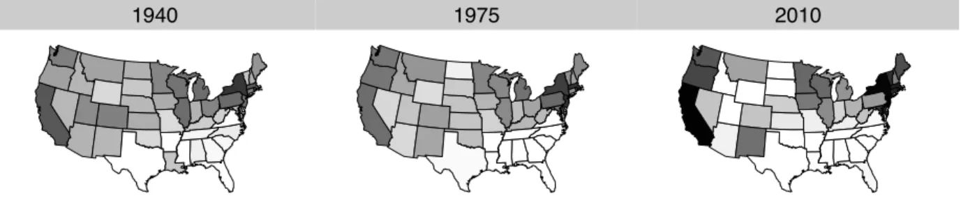
1940 1975 2010
Figure 1: The geographic distribution of government policy liberalism in 1940, 1975, and 2010. Darker shading indicates liberalism; lighter shading indicates conservatism. The esti-mates have been centered and standardized in each year to accentuate the shading contrasts. have become substantially more liberal, especially between the 1930s and 1970s.15 We use a
time-varying model instead because it helps avoid the interpretational difficulties of assum-ing that policies have the same substantive meanassum-ing across long stretches of time. The price of this flexibility is that states’ policy liberalism scores are comparable over time primarily in a relative sense.
Figure 1 maps state policy liberalism in 1940, 1975, and 2010. As is clear from this figure, the geographic distribution of policy liberalism has remained remarkably stable, despite huge changes in the distribution of mass partisanship, congressional ideology, and other political variables over past seven decades. Throughout the period, Southern states had the most conservative policies. This holds not only on civil rights, but on taxes, welfare, and a host of social issues. By contrast, the most liberal states have consistently been in the Northeast, Pacific, and Great Lakes regions. New York, for example, has consistently had the most liberal tax and welfare policies in the nation, and it was also among the first states to adopt liberal policies on cultural issues such as abortion, gun control, and gay rights.
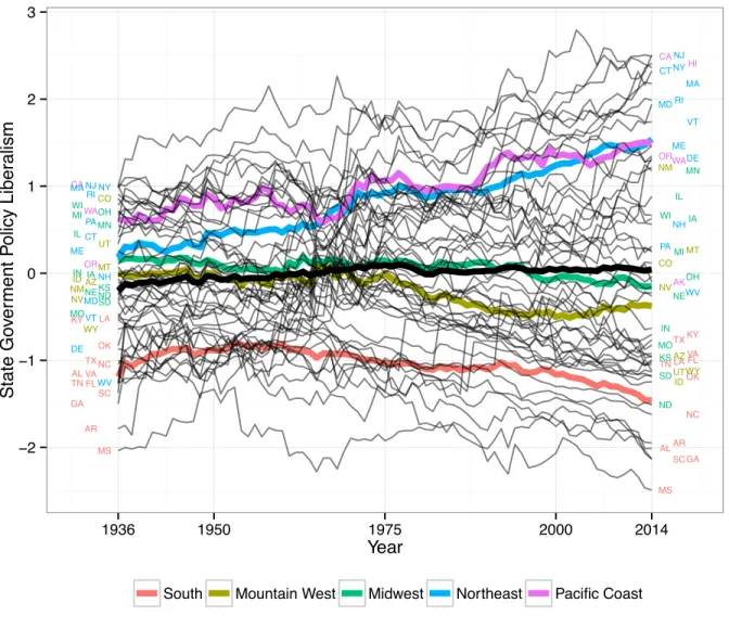
The overall picture of aggregate stability, however, masks considerable year-to-year fluc-tuation in policy liberalism as well as major long-term trends in certain states. These details can be discerned more easily in Figure 2, which plots the yearly time series of individual states
15. In these years, U.S. states expanded their welfare responsibilities and tax bases while loosening a variety of social restrictions. This aggregate trend towards more liberal policies largely ceased after 1980.
AL AR AZ CA CO CT DE FL GA IA ID IL IN KS KY LA MA MD ME MI MN MO MS MT NC ND NE NH NJ NM NV NY OH OK OR PA RI SC SD TN TX UT VA VT WA WI WV WY AK ALAR AZ CA CO CT DE FL GA HI IA ID IL IN KS KY LA MA MD ME MI MN MO MS MT NC ND NE NH NJ NM NV NY OH OK OR PA RI SC SD TN TX UT VA VT WA WI WV WY −2 −1 0 1 2 3 1936 1950 1975 2000 2014 Year State Go ver ment P olicy Liber alism
South Mountain West Midwest Northeast Pacific Coast
Figure 2: State government policy liberalism, 1936–2014. The thicker black line tracks the mean in each year, and the colored lines indicate the means in five geographic regions.
between 1936 and 2014. Due to explicit policy revisions as well as to policy “drift” relative to other states, policy liberalism can change substantially between years, though cross-sectional di↵erences between states are generally much larger than within-state changes. The variance across states has also increased over time, possibly due to growing geographic polarization.
Figure 2 also shows that not all states have been ideologically stable. The policies of Northeastern states became steadily more liberal over this time period. Whereas states like Delaware, Maryland, and Vermont were once more conservative than average, by 2014 all three had joined most of the rest of the Northeast in the top quartile of liberalism. Their early adoption of gay marriage and other rights for homosexuals, for example, contrasts with their slowness in passing racial anti-discrimination laws in the 1950s and 1960s. The welfare benefits and regulatory policies of these states exhibited a similar liberalizing trajectory.
Several Midwestern, Mountain, and Southern states have followed the opposite trajectory. Idaho, for example, became much more conservative over this period. In the 1930s–1950s, Idaho actually had some of the most generous welfare benefits in the nation, but by the early 2000s they were among the least generous. Louisiana too has shifted substantially to the right. In the 1930s, Louisiana’s welfare benefits were the most generous in the South and roughly equivalent to those of several Northern states, but they gradually become less generous over the next few decades. Louisiana also waited longer than any other Southern state to pass a durable right-to-work law, but it finally did so in 1976.16
These states’ shifts in policy liberalism track the evolution of their presidential partisan-ship. For instance, in the presidential election of 1936, the first year in our dataset, Maine, Vermont, and New Hampshire were the three most Republican states in the nation, but by 2012 all three (especially Vermont) were more Democratic than average. The opposite is true of the Mountain West, which transformed from Democratic-leaning to solidly Republican. On the whole, the 2010 map in Figure 1 matches contemporaneous state partisanship much
16. Louisiana passed a right-to-work law in 1954 but repealed it in 1956, when the populist Long faction of the Democratic Party recaptured control of state government (Canak and Miller 1990). The unusual power of this faction, forged by Governor and Senator Huey Long in the late 1920s, may help explain Louisiana’s anomalously (for the region) liberal state policies in that era (Key 1949, 156–82).
better than the earlier maps, primarily because the South’s shift to the Republicans finally aligned its partisanship to match its consistently conservative state policies.
Measurement Validity
Having illustrated the face validity of the policy liberalism estimates, we now conduct a more systematic validation of our measure. We begin with convergent validation (Adcock and Collier 2001), documenting the very strong cross-sectional relationships between our estimates’ and existing measures of policy liberalism. We then turn to construct validation, demonstrating that our policy liberalism scale is also highly correlated with measures of theoretically related concepts, such as presidential partisanship. Finally, we show that our policy liberalism scale is strongly related to domain-specific policy measures, and that the predictive fit of the model barely increases if a second dimension is added to the measure-ment model. Overall, this evidence corroborates our claim that a one-dimensional model adequately captures the systematic variation in state policies, and that this dimension is properly interpreted as policy liberalism.
Convergent Validation
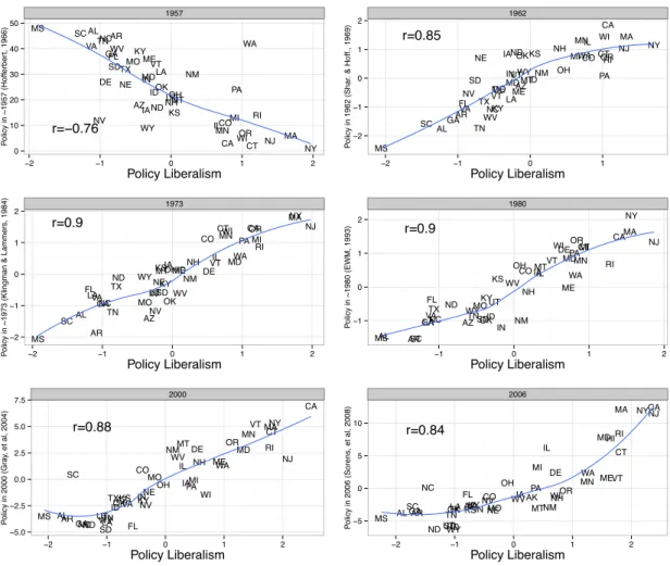
If our estimates provide a valid measure of policy liberalism, they should be strongly related to other (valid) measures of the same concept. Since ours is the first time-varying measure of state policy liberalism, we must content ourselves with examining the cross-sectional relationship between our measure and ones developed by other scholars at various points in time. Figure 3 plots the cross-sectional relationships between our measure of policy liberalism and six existing measures:
• “liberalness”/“welfare orientation” rank circa 1957 (Ho↵erbert 1966)17
• welfare-education liberalism in 1962 (Sharkansky and Ho↵erbert 1969)18
17. This index is based on mean per-recipient expenditures for 1952–61 for aid to the blind, old age assistance, unemployment compensation, expenditure for elementary and secondary education, and aid to dependent children. We compare Ho↵erbert’s (1966) scale with our measure of state policy liberalism in 1957 since this is the midpoint of the years he includes in his index.
AL AR AZ CA CO CT DE FL GA IA ID IL IN KS KY LA MA MD ME MI MN MO MS MT NC ND NE NH NJ NM NV NY OH OK OR PA RI SC SD TN TX UT VA VT WA WI WV WY r=−0.76 1957 0 10 20 30 40 50 −2 −1 0 1 2 Policy Liberalism P olicy in ~1957 (Hoff erber t, 1966) AL AR AZ CA CO CT DE FL GA IA ID IL IN KS KY LA MA MD ME MI MN MO MS MT NC ND NE NH NJ NM NV NY OH OK OR PA RI SC SD TN TX UT VA VT WA WI WV WY r=0.9 1973 −2 −1 0 1 2 −2 −1 0 1 2 Policy Liberalism P
olicy in ~1973 (Klingman & Lammers
, 1984) ALAR AZ CA CO CT DE FL GA IA ID IL IN KS KY LA MA MD ME MI MN MO MS MT NCND NE NH NJ NM NV NY OH OK OR PA RI SC SD TN TX UT VA VT WA WI WV WY r=0.88 2000 −5.0 −2.5 0.0 2.5 5.0 7.5 −2 −1 0 1 2 Policy Liberalism P olicy in 2000 (Gr a y, et al, 2004) AL AR AZ CA CO CT DE FL GA IA ID IL IN KS KYLA MA MD ME MI MN MO MS MT NC ND NE NH NJ NM NV NY OH OK OR PA RI SC SD TN TX UT VA VT WA WI WV WY r=0.85 1962 −2 −1 0 1 2 −2 −1 0 1 Policy Liberalism P olicy in 1962 (Shar . & Hoff ., 1969) AL AR AZ CA CO CT DE FL GA IA ID IL IN KS KY LA MA MD ME MI MN MO MS MT NC ND NH NJ NM NY OH OK OR PA RI SC SD TN TX UT VA VT WA WI WV WY r=0.9 1980 −1 0 1 2 −1 0 1 2 Policy Liberalism P olicy in ~1980 (EWM, 1993) AK AL AR AZ CA CO CT DE FL GA HI IA ID IL IN KSKY LA MA MD ME MI MN MO MS MT NC ND NE NH NJ NM NV NY OH OK OR PA RI SC SD TNTX UT VA VT WA WI WV WY r=0.84 2006 −5 0 5 10 −2 −1 0 1 2 Policy Liberalism P olicy in 2006 (Sorens , et al, 2008)
Figure 3: Convergent validation: relationships between our policy liberalism estimates and six existing measures. Fitted lines indicate loess curves.
• policy liberalism circa 1973 (Klingman and Lammers 1984)19
• policy liberalism circa 1980 (Wright, Erikson, and McIver 1987)20
• policy liberalism in 2000 (Gray et al. 2004)21
also includes several social outcomes, such as school graduation rates.
19. This index is based on data measured at a variety of points between 1961 and 1980 on state innovative-ness, anti-discrimination policies, monthly payments for Aid to Families with Dependent Children (AFDC), the number of years since ratification of the Equal Rights Amendment for Women, the number of consumer-oriented provisions, and the percentage of federal allotment to the state for Title XX social services programs actually spent by the state. We compare Klingman and Lammers’s (1984) scale with our measure of state policy liberalism in 1973 since this is the midpoint of the years they include in their index.
20. This measure is based on state education spending, the scope of state Medicaid programs, consumer protection laws, criminal justice provisions, whether states allowed legalized gambling, the number of years since ratification of the Equal Rights Amendment for Women, and the progressivity of state tax systems. We compare Wright, Erikson, and McIver’s (1987) scale with our measure of state policy liberalism in 1980 since this is roughly the midpoint of the years they include in their index.
21. This index is based on state firearms laws, state abortion laws, welfare stringency, state right-to-work laws, and the progressively of state tax systems.
• policy liberalism in 2006 (Sorens, Muedini, and Ruger 2008)22
Each panel plots the relationship between our policy liberalism estimates (horizontal axis) and one of the six existing measures listed above. A loess curve summarizes each relationship, and the bivariate correlation is given on the left side of each panel.
Notwithstanding measurement error and di↵erences in data sources, our estimates are highly predictive of other measures of policy liberalism. The weakest correlation, 0.76 for Ho↵erbert (1966), is primarily the result of a few puzzling outliers (Washington, for example, is the seventh-most conservative state on Ho↵erbert’s measure, whereas Wyoming is the ninth-most liberal). In addition, all the relationships are highly linear. The only partial exception is for Sorens, Muedini, and Ruger (2008), whose measure of policy liberalism does not discriminate as much between Southern states as our measure, resulting in a flat relationship at the conservative end of our scale.
In short, the very strong empirical relationships between our policy liberalism scale and existing measures of the same concept provide compelling evidence for the validity of our measure. It is worth noting that most of the existing scales were constructed explicitly with the goal of di↵erentiating between liberal and conservative states. Thus their tight relation-ship with our measure, which is based on a much more comprehensive policy dataset and was estimated without regard to the ideological content of the policy indicators,23 suggests
in particular that we are on firm ground in calling our latent dimension “policy liberalism.”
Construct Validation
The purpose of construct (a.k.a. “nomological”) validation is to demonstrate that a mea-sure conforms to well-established hypotheses relating the concept being meamea-sured to other concepts (Adcock and Collier 2001, 542–3). One such hypothesis is that the liberalism of a state’s policies is strongly related to the liberalism of its state legislature, though due to
22. This is the first principal component uncovered by Sorens, Muedini, and Ruger’s (2008) analysis of over 100 state policies. They label this dimension “policy liberalism” and give the label “policy urbanism” to the second principal component.
factors such as legislative gridlock the relationship may not be perfect (e.g., Krehbiel 1998). To measure legislative liberalism on a common scale, we rely on Shor and McCarty’s (2011) estimates of the conservatism of members of state legislative lower houses. As Figure 4 demonstrates for presidential years between 1996 and 2008, states with more liberal policies tend to have more liberal median legislators. Due possibly to the lingering Democratic ad-vantage in Southern state legislatures, the relationship at the conservative end of the policy spectrum is fairly flat, though by 2008 the relationship had become much more linear. The correlation between legislative conservatism and policy liberalism has also strengthened over time, from 0.51 in 1996 to 0.80 in 2008. AK AL AZ CA CO CT DE FL GA HI IA ID IL IN KS KY LA MA MD ME MI MN MO MS NC NH NJ NM NY OH OK PA RI SC SD TN TX UT VA VT WA WI WV WY r=−0.51 AK AK AL ALARAR AZ AZ CA CA CO CO CT CT DE DE FL FL GA GA HI IA IA ID ID IL IL IN IN KS KS KY KY LA LA MA MA MD MD ME ME MI MI MN MN MO MO MS MS MT MT NC NC ND ND NH NH NJ NJ NM NM NV NV NY NY OH OH OK OK PAPA OROR RI RI SC SC SDSD TN TN TX TX UT UT VA VA VT VT WA WA WI WI WV WV WY WY r=−0.56 AK ALAR AZ CA CO CT DE FL GA HI IA ID IL IN KS KY LA MA MD ME MI MN MO MS MT NC ND NH NJ NM NV NY OH OK OR PA RI SC TN TX UT VA VT WA WI WV WY r=−0.69 AK AL AR AZ CA CO CT DE FL GA HI IA ID IL IN KS KY LA MD ME MI MN MO MS MT NC ND NH NJ NY OH OR PA RI SC SD TN TX VA WA WI WV WY r=−0.8 1996 2000 2004 2008 −1.0 −0.5 0.0 0.5 −1.0 −0.5 0.0 0.5 −1.5 −1.0 −0.5 0.0 0.5 −1.5 −1.0 −0.5 0.0 0.5 −2 −1 0 1 2 −2 −1 0 1 2 −2 −1 0 1 2 −2 −1 0 1 2 Policy Liberalism
Median Legislator in State House (Shor & McCar
ty
, 2011)
Figure 4: The relationship between state policy liberalism and the conservatism of the median member of the lower house of the state legislature (Shor and McCarty 2011), 1996–2008.
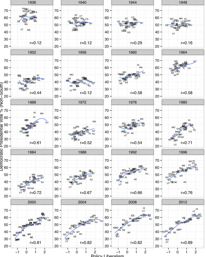
An analogous pattern of increasing association over time can be seen in an examination of the relationship between policy liberalism and Democratic presidential vote share. It is natural to hypothesize that both presidential vote and state policy liberalism are responsive
to the party and policy preferences of mass publics and thus should be correlated at the state level. Since the anomalously Democratic partisanship of the “Solid South” would distort this relationship, we focus on the non-South only. Even without Southerns states, however, pol-icy liberalism and presidential vote are only weakly related in the early part of the period, as Figure 5 shows. The correlation jumped to 0.58 in 1960 and continued to increase grad-ually through 2012, when it reached nearly 0.9. This increasing association between policy liberalism and presidential vote mirrors the growing alignment of party identification, pol-icy preferences, and presidential vote at the mass level (Fiorina and Abrams 2008, 577–82). The analysis of presidential vote thus provides further evidence for the validity of our pol-icy liberalism scale. At same time, however, it suggests the limitations of presidential vote share as a proxy for mass preferences before the 1960s, even in the non-South (contra, e.g., Canes-Wrone, Brady, and Cogan 2002).
Finally, we examine the relationship between our policy liberalism measure and its clos-est analogue, Jacoby and Schneider’s (2009) policy priorities scale. As we emphasize above, policy liberalism and policy priorities are di↵erent concepts. Moreover, the theoretical rela-tionship between policy liberalism and preference for collective over particularistic spending is not self-evident. Nevertheless, Jacoby and Schneider convincingly argue that in U.S. states tend to target particularized policies at needy constituencies. Consistent with that expec-tation, they find a moderately negative cross-sectional correlation between policy liberalism and preference for collective goods.
Based on a similar analysis, we too find policy liberalism and policy priorities to be negatively correlated, on the order of 0.5. As Figure 6 shows, their relationship atten-uated somewhat between 1982 and 2005. Also, like Jacoby and Schneider (2009, 18–20), we find that non-linearity in the measures’ relationship contributes to the weak correlation: their association is much stronger among relatively liberal and particularistic states than on the conservative/collective-good end of the spectrum. This seems to be driven in part by Southern states, which always anchor the conservative end of our scale but seem to favor
par-AZ CA CO CT DE IA ID IL IN KS MA MD ME MI MN MO MT ND NE NH NJ NM NV NY OH OR PA RI SD UT VT WAWI WY r=0.12 AZ CA CO CT DE IA ID IL IN KS MA MD ME MIMN MO MT ND NE NH NJ NM NV NY OH OR PA RI SD UT VT WA WI WY r=0.12 AZ CA CO CT DE IA ID IL IN KS MA MD ME MI MN MO MT ND NE NHNM NJ NV NY OH ORPA RI SD UT VT WA WI WY r=0.29 AZ CA CO CT DE IAIDIN IL KS MA MD ME MI MN MO MT ND NE NH NJ NM NV NY OH OR PA RI SD UT VT WA WI WY r=0.16 AZ CA CO CT DE IA ID IL IN KS MA MD ME MI MN MO MT ND NE NH NJ NM NV NY OH OR PARI SD UT VT WA WI WY r=0.44 AZ CA CO CT DE IAINID IL KS MA MD ME MI MN MO MT ND NE NH NJ NM NV NY OH ORPA RI SD UT VT WA WI WY r=0.12 AK AZ CA CO CT DE HI IAID IL IN KS MA MD ME MI MN MO MT ND NE NH NJ NM NV NY OH OR PA RI SD UT VT WAWI WY r=0.58 AK AZ CA CO CT DEIA ID IL INKS MD ME MI MN MO MT ND NE NH NJ NM NV NY OH ORPA SD UT VT WA WI WY r=0.58 AK AZ CA CO CT DE HI IA ID IL IN KS MA MD ME MI MN MO MT ND NE NH NJ NM NV NY OHOR PA RI SD UT VT WA WI WY r=0.61 AK AZ CA CO CT DE HI IA ID IL IN KS MA MD ME MI MN MOMT ND NE NH NJ NM NV NY OH OR PA RI SD UT VT WA WI WY r=0.52 AK AZ CA CO CT DE HI IA ID IL IN KS MA MD ME MI MN MO MT ND NE NH NJ NM NV NY OH ORPA RI SD UT VT WA WI WY r=0.54 AK AZ CA CO CT DE HI IA ID IL IN KS MA MD MEMI MN MO MT ND NE NH NJ NM NV NY OH ORPA RI SD UT VT WA WI WY r=0.71 AK AZ CA CO CT DE HI IA ID IL IN KS MA MD MEMI MN MO MT ND NENH NJ NM NV NY OH OR PA RI SD UT VTWA WI WY r=0.72 AK AZ CA CO CT DE HI IA ID IL IN KS MA MD MEMI MN MO MT ND NE NH NJ NM NV NY OH OR PA RI SD UT VT WAWI WY r=0.67 AK AZ CA CO DE CT HI IA ID IL IN KS MA MD MEMIMN MO MT ND NE NH NJ NM NV NY OH OR PA RI SD UT VT WA WI WY r=0.66 AK AZ CA CO CT DE HI IA ID IL IN KS MA MD ME MI MN MO MT ND NE NH NJ NM NV NY OHPAOR RI SD UT VT WA WI WY r=0.76 AK AK AZ AZ CA CA CO CO CT CT DE DE HI IA IA ID ID IL IL IN IN KS KS MA MA MD MD ME ME MI MI MNMN MO MO MT MT ND ND NENE NH NH NJ NJ NM NM NV NV NY NY OH OH OROR PA PA RI RI SD SD UT UT VT VT WA WA WI WI WY WY r=0.81 AK AZ CA CO CT DE HI IA ID IL IN KS MA MD ME MI MN MO MT ND NE NHNM NJ NV NY OH OR PA RI SD UT VT WA WI WY r=0.82 AK AZ CA CO CT DE HI IA ID IL IN KS MA MD ME MI MN MO MT ND NE NHNM NJ NV NY OH OR PA RI SD UT VT WA WI WY r=0.82 AK AZ CA CO CT DE HI IA ID IL IN KS MA MD ME MI MN MO MT ND NE NH NJ NM NV NY OH OR PA RI SD UT VT WA WI WY r=0.89 1936 1940 1944 1948 1952 1956 1960 1964 1968 1972 1976 1980 1984 1988 1992 1996 2000 2004 2008 2012 20 30 40 50 60 70 20 30 40 50 60 70 20 30 40 50 60 70 20 30 40 50 60 70 20 30 40 50 60 70 20 30 40 50 60 70 20 30 40 50 60 70 20 30 40 50 60 70 20 30 40 50 60 70 20 30 40 50 60 70 20 30 40 50 60 70 20 30 40 50 60 70 20 30 40 50 60 70 20 30 40 50 60 70 20 30 40 50 60 70 20 30 40 50 60 70 20 30 40 50 60 70 20 30 40 50 60 70 20 30 40 50 60 70 20 30 40 50 60 70 −1 0 1 2 −1 0 1 2 −1 0 1 2 −1 0 1 2 Policy Liberalism Democr atic Presidential V ote % (Non − South)
Figure 5: The relationship between state policy liberalism and Democratic presidential vote share, 1936–2012 (non-South only).
ticularistic spending. The sources of this discrepancy between the two measures—perhaps di↵erences in political culture, budgetary decentralization, or economic need—could be an interesting topic for future research.
AK AL AR AZ CA CO CT DE FL GA IA ID IL IN KSKY LA MA MD ME MI MN MO MS MT NC ND NE NH NJ NM NV NY OH OK OR PA RI SC SD TN TX UT VA VT WA WI WV WY r=−0.57 AK AL AR AZ CA CO CT DE FL GA IA ID IL IN KS KY LA MA MD ME MI MN MO MS MT NCND NE NH NJ NM NV NY OH OK OR PA RI SC SD TN TX UTVA VT WA WI WV WY r=−0.55 AK AL AR AZ CA CO CT DE FL GA IA ID IL IN KS KY LA MA MD ME MI MN MO MS MT NC ND NE NH NJ NM NV NY OH OK OR PA RI SC SD TN TX UT VA VT WA WI WV WY r=−0.44 AK AL AR AZ CA CO CT DE FL GA IA ID IL IN KS KY LA MA MD ME MI MN MO MS MT NC ND NE NH NJ NM NV NY OH OK OR PA RI SC SD TN TX UT VA VT WA WI WV WY r=−0.33 1982 1990 1998 2005 −0.2 −0.1 0.0 0.1 0.2 −0.2 −0.1 0.0 0.1 0.2 −2 −1 0 1 2 −2 −1 0 1 2 Policy Liberalism P olicy Pr ior ities (J acob y & Schneider , 2009)
Figure 6: The relationship between policy liberalism and policy priorities (Jacoby and Schnei-der 2009) in selected years, 1982–2005.
Dimensionality
Our one-dimensional model of state policies implies that a single latent trait captures system-atic policy variation across states. This is not to say that it captures all policy di↵erences, but it does imply that once policies’ characteristics and states’ policy liberalism are ac-counted for, any additional variation in state policies is essentially random. This assumption would be violated if there were instead multiple dimensions of state policy, as some
schol-ars have claimed. Given that roll-call alignments in the U.S. Congress were substantially two-dimensional for much of the 20th century (Poole and Rosenthal 2007), it is not un-reasonable to suspect that state policies might be as well. As we demonstrate, however, a one-dimensional model captures state policy variation surprisingly well, and there is little value to increasing the complexity of the model by adding further dimensions.
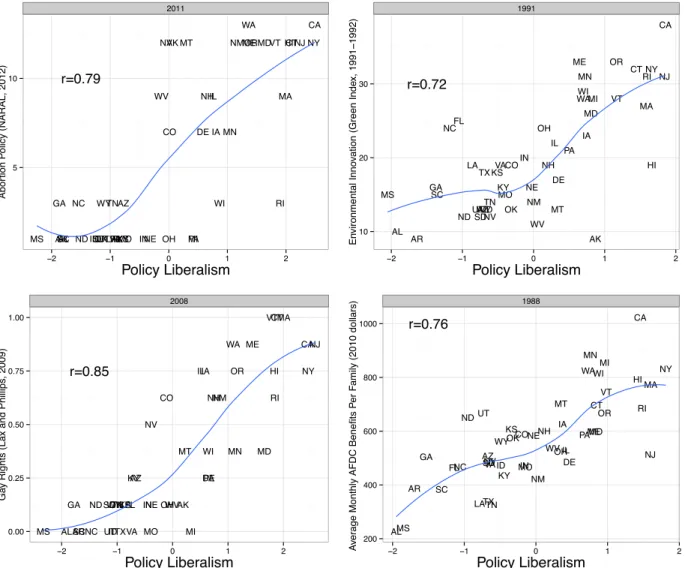
AK AL AR AZ CA CO CT DE FL GA HI IA ID IL IN KS KY LA MA MD ME MI MN MO MS MT NC ND NE NH NJ NM NV NY OH OK OR PA RI SC SD TN TX UTVA VT WA WI WV WY r=0.79 2011 5 10 −2 −1 0 1 2 Policy Liberalism Abor tion P olicy (NARAL, 2012) AK ALAR AZ CA CO CT DE FL GA HI IA ID IL IN KS KY LA MA MD ME MI MN MO MS MT NC ND NE NH NJ NM NV NY OH OK OR PA RI SC SDTN TX UT VA VT WA WI WV WY r=0.85 2008 0.00 0.25 0.50 0.75 1.00 −2 −1 0 1 2 Policy Liberalism Ga
y Rights (Lax and Phillips
, 2009) AK AL AR AZ CA CO CT DE FL GA HI IA ID IL IN KS KY LA MA MD ME MI MN MO MS MT NC ND NE NH NJ NM NV NY OH OK OR PA RI SC SD TN TX UT VA VT WAWI WV WY r=0.72 1991 10 20 30 −2 −1 0 1 2 Policy Liberalism En vironmental Inno
vation (Green Inde
x, 1991 − 1992) AL AR AZ CA CO CT DE FL GA HI IA ID IL IN KS KY LA MA MD ME MI MN MO MS MT NC ND NENH NJ NM NV NY OH OK OR PA RI SC SD TN TX UT VA VT WAWI WV WY r=0.76 1988 200 400 600 800 1000 −2 −1 0 1 2 Policy Liberalism A ver
age Monthly AFDC Benefits P
er F
amily (2010 dollars)
Figure 7: Relationships between policy liberalism and four issue-specific scales (abortion rights, environmental protection, gay rights, and welfare benefits).
One fact in support for unidimensionality is that the most discriminating policies in our dataset—those most strongly related to the latent factor—span a wide range of issues, in-cluding racial discrimination, women’s rights, gun control, labor law, energy policy, criminal
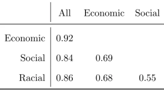
Table 1: Correlations between policy liberalism scales estimated using economic, social, racial, and all policies. The unit of analysis is the state-year. The racial policy scale is estimated for the 1950–70 period only.
All Economic Social Economic 0.92
Social 0.84 0.69
Racial 0.86 0.68 0.55
rights, and welfare policy. Additional evidence is provided by the relationships between pol-icy liberalism and four issue-specific scales: NARAL’s abortion rights scale (NARAL 2012), the Green Index of Environmental Innovation in 1991–92 (Hall and Kerr 1991; Ringquist and Garand 1999), a gay rights index derived from Lax and Phillips (2009b), and average AFDC benefits per family in each state (Moffitt 2002). As Figure 7 shows, policy liberalism accurately predicts variation within each of these disparate policy areas.
We can explore this question at a higher level of generality by scaling state policies within each of three broad issue domains: economic, social, and racial.24 Policy cleavages in the
mass public and in the U.S. Congress are often considered to di↵er across these domains, especially earlier in the 1936–2014 period (e.g., Layman, Carsey, and Horowitz 2006; Poole and Rosenthal 2007). As the first column of the correlation matrix in Table 1 shows, however, each domain-specific scale is strongly related to the policy liberalism scale based on all policies. The domain-specific scales are also highly correlated with each other, with the correlation being weakest for racial and social policies (estimated for 1950–70 only). On the whole, Table 1 provides strong evidence that variation in state policies is one-dimensional and does not vary importantly across issue domains.
As a final piece of evidence, we show that allowing for multiple latent dimensions does not
24. Because cross-state variation in civil rights policies is concentrated in the 1950–70 period, we estimate the racial policy dimension for these two decades only.
substantially improve our ability to predict policy di↵erences between states. As our measure of model fit we use percentage correctly predicted (PCP), which for binary variables is the percentage of cases for which the observed value corresponds to its model-based predicted value (0 or 1). In order to include ordinal and continuous variables in this calculation, we convert them into binary variables by dichotomizing them at a threshold randomly generated for each variable. We estimate one and two-dimensional probit IRT models separately in each year using the R function ideal (Jackman 2012), which automatically calculates PCP. We then evaluate how much the second dimension improves PCP (adding dimensions cannot decrease PCP).
Based on this method, we find little evidence that adding dimensions improves our ability to account for the data. In the average year, a one-dimensional model correctly classifies 82% of all dichotomized policy observations. Adding a second dimension increases average PCP by only 1.5 percentage points. This improvement in model fit is less than the increase in fit that is used in the congressional literature as a barometer of whether roll-call voting in Congress has a one-dimensional structure (Poole and Rosenthal 2007, 33–4). Further, the minimal improvement in model fit gained from adding a second dimension is consistent across time—even during the mid-century heyday of two-dimensional voting in Congress.
Taken as a whole, the evidence supports two conclusions. First, a single latent dimension captures the vast majority of policy variation across states across disparate policy domains. This is true even at times when national politics was multidimensional. Second, the approxi-mately 20% of cross-sectional policy variation not captured by a one-dimensional model does not seem to have a systematic structure to it, or at least not one that can be described by additional dimensions.
Substantive Applications
Our dynamic measure of policy liberalism opens up multiple avenues of research not possible with cross-sectional measures. Most obviously, as we have shown, it permits descriptive
analyses of the ideological evolution of state policies over long periods of time. But the availability of a dynamic measure also facilitates causal analyses that incorporate policy liberalism as an outcome, treatment, or control variable. In particular, because it is available for each state-year, our measure can be used in time-series–cross-sectional (TSCS) research designs, which leverage variation across both units and time. The fact that our estimates are available for nearly 80 years is especially valuable because TSCS estimators can perform poorly unless the number of time units is large (e.g., Nickell 1981).
For example, scholars could examine how the cross-sectional relationship between state public opinion and policy liberalism has evolved over time (Burstein 2003); estimate the state-level relationship between changes in opinion and changes in policy (cf. Stimson, MacKuen, and Erikson 1995); or analyze how interest groups or electoral institutions moderate the opinion–policy link (cf. Gray et al. 2004; Lax and Phillips 2011). Or scholars could evaluate the policy e↵ects of electoral outcomes or the partisan composition of state government (cf. Erikson, Wright, and McIver 1989; T. Kousser 2002; Besley and Case 2003; Leigh 2008). An alternative approach would be to analyze policy liberalism as a cause rather than an e↵ect. For example, one prominent view is that citizens respond“thermostatically”to changes in policy by moving in the ideologically opposite direction (Wlezien 1995). A related perspec-tive argues that voters compensate for partisan e↵ects on policy through partisan balancing (e.g., Erikson 1988; Alesina, Londregan, and Rosenthal 1993). Other scholars, however, highlight the positive feedback e↵ects of policy changes (e.g., Pierson 1993; Campbell 2012). Our policy liberalism estimates open up ways of adjudicating among these theories using state-level TSCS designs.
The Policy E↵ects of Voter Registration Reforms
To illustrate the kinds of analyses made possible by our estimates, we conduct a brief inves-tigation into the policy e↵ects of reforms designed to make voter registration easier. While debate over such reforms often focuses on e↵ects on turnout or partisan advantage, their
ef-fects on policy are arguably most important.25 One intuitive theoretical prediction, derived
from median-voter models of redistribution, is that lowering registration barriers makes the electorate larger and poorer, which in turn increases political support for redistributive (i.e., liberal) policies (Meltzer and Richard 1981; Husted and Kenny 1997).
The policy consequences of registration regulations specifically have been examined by Besley and Case (2003, 35–7), who using a fixed-e↵ect (FE) framework find liberalizing e↵ects of lower registration barriers on five state taxation and spending policies in the period 1958–98. Besley and Case’s two-way FE specification improves substantially over cross-sectional comparisons, which cannot control for unobserved di↵erences between states. An important weakness of their specification, however, is that it assumes that states did not trend in di↵erent directions over the period they examine.26 Figure 2 suggests, however,
that this assumption is false (see, e.g., the liberalizing trend among Northeastern states). The likely consequence is that Besley and Case’s e↵ect estimates are much too large.
We replicate and extend Besley and Case’s analysis, examining the policy e↵ects of three electoral policies—“motor voter” laws, election-day registration, and mail-in registration—on state policy liberalism between 1950 and 2000.27 To guard against di↵erential time trends,
we use a more conservative specification that includes a lagged dependent variable (LDV) as well as state and year FEs.28 One advantage of a long time series is the finite-sample
bias of LDV-FE models is of order 1/T and thus decreases rapidly as the number of time
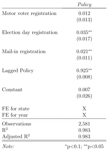
units increases (Beck and Katz 2011, 342). Table 2 reports the estimated e↵ect estimates, all of which are positive and, except for motor voter registration, distinguishable from 0. In terms of substantive magnitude, these estimates imply that making voter registration easier increases the probability of a state adopting a liberal law by about 1 percentage point.
25. See, for example, Key’s (1949) and J. M. Kousser’s (1974) analyses of the policy e↵ects of su↵rage restrictions in the post-Reconstruction South.
26. Besley and Case (2003) do include a few time-varying demographic controls, but these are unlikely to account for di↵erential state trends.
27. We obtained data on the first two policies from Besley and Case (2003) and data on the third from Springer (2014).
28. Following Besley and Case (2003), we define a unit-year as “treated” by a registration policy if that policy was in e↵ect at the last election.
Consistent with our concern about state-specific trends, the estimates from a simple two-way FE model (not shown) are all an order of magnitude larger than their LDV-FE counterparts.
Table 2: E↵ect of Electoral Reforms on State Policy Liberalism Policy
Motor voter registration 0.012 (0.013) Election day registration 0.035⇤⇤
(0.017) Mail-in registration 0.021⇤⇤ (0.011) Lagged Policy 0.925⇤⇤ (0.008) Constant 0.007 (0.026) FE for state X FE for year X Observations 2,581 R2 0.983 Adjusted R2 0.983 Note: ⇤p<0.1; ⇤⇤p<0.05
Though brief, this application highlights several advantages of our measure of policy lib-eralism. First, its TSCS structure enables us to exploit within-state variation in institutions such as registration regulation. Second, its long time series permits the use of estimators, such as LDV-FE models, whose performance improves as T increases. Third, the precision of our composite measure relative to any individual indicator of liberalism means allows us to detect small but meaningful e↵ects, such as the ones reported in Table 2.
Conclusion
This paper has addressed a major gap in the state politics literature: the lack of a measure of state policy liberalism that varies across time. Using a dataset covering 148 policies and a latent-variable model designed for a mix of ordinal and continuous data, we have generated estimates of the policy liberalism of every state in every year for the past three-quarters of a century. As indicated by their high correlations with existing measures of state policy liberalism as well as with domain-specific indices, our estimates exhibit strong evidence of validity as a measure of policy liberalism.
Our yearly estimates of policy liberalism are illuminating for their own sake, revealing historical patterns in the development of state policymaking that would be hard to discern otherwise. But they also open up research designs that leverage temporal variation in state policies to explore questions involving the causes and e↵ects of policy outcomes. These topics include the policy e↵ects of public mood, electoral outcomes, interest groups, and institutions, as well as the consequences of policy change on political attitudes and behavior. The relevance of this paper extends well beyond the field of state politics. In addition to facilitating the study of topics of general significance, our measurement model could be ap-plied to policymaking by local governments (cf. Tausanovitch and Warshaw 2014) as well as in cross-national studies. Even more generally, our dynamic approach to measurement helps to illustrate the value of data-rich, time-varying measures of important political concepts like policy liberalism.
References
Adcock, Robert, and David Collier. 2001. “Measurement Validity: A Shared Standard for Qualitative and Quantitative Research.” American Political Science Review 95 (3): 529– 546.
Alesina, Alberto, John Londregan, and Howard Rosenthal. 1993. “A Model of the Political Economy of the United States.” American Political Science Review 87 (1): 12–33. Ansolabehere, Stephen, Jonathan Rodden, and James M. Snyder Jr. 2008. “The Strength of
Issues: Using Multiple Measures to Gauge Preference Stability, Ideological Constraint, and Issue Voting.” American Political Science Review 102 (2): 215–232.
Bafumi, Joseph, Andrew Gelman, David K. Park, and Noah Kaplan. 2005. “Practical Issues in Implementing and Understanding Bayesian Ideal Point Estimation.” Political Analysis 13 (2): 171–187.
Beck, Nathaniel, and Jonathan N. Katz. 2011. “Modeling Dynamics in Time-Series–Cross-Section Political Economy Data.” Annual Review of Political Science 14 (1): 331–352. Berry, William D., Richard C. Fording, and Russell L. Hanson. 2000. “An Annual Cost of
Living Index for the American States, 1960–1995.” Journal of Politics 62 (2): 550–567. Besley, Timothy, and Anne Case. 2003. “Political Institutions and Policy Choices: Evidence
from the United States.” Journal of Economic Literature 41 (1): 7–73.
Burstein, Paul. 2003. “The Impact of Public Opinion on Public Policy: A Review and an Agenda.” Political Research Quarterly 56 (1): 29–40.
Campbell, Andrea Louise. 2012. “Policy Makes Mass Politics.” Annual Review of Political Science 15:333–351.
Canak, William, and Berkeley Miller. 1990.“Gumbo Politics: Unions, Business, and Louisiana Right-to-Work Legislation.” Industrial and Labor Relations Review 43 (2): 358–271.
Canes-Wrone, Brandice, David W. Brady, and John F. Cogan. 2002. “Out of Step, Out of Office: Electoral Accountability and House Members’ Voting.” American Political Science Review 96 (1): 127–140.
Chandler, Marsha, William Chandler, and David Vogler. 1974. “Policy Analysis and the Search for Theory.” American Politics Research 2 (1): 107–118.
Clinton, Joshua, Simon Jackman, and Douglas Rivers. 2004. “The Statistical Analysis of Roll Call Data.” American Political Science Review 98 (2): 355–370.
Converse, Philip E. 1964. “The Nature of Belief Systems in Mass Publics.” In Ideology and Discontent, edited by David E. Apter, 206–261. London: Free Press.
Elazar, Daniel Judah. 1966. American Federalism: A View from the States. New York: Crow-ell.
Ellis, Christopher, and James A. Stimson. 2012. Ideology in America. New York: Cambridge UP.
Erikson, Robert S. 1988. “The Puzzle of Midterm Loss.” Journal of Politics 50 (4): 1011– 1029.
Erikson, Robert S., Gerald C. Wright, and John P. McIver. 1989. “Political Parties, Public Opinion, and State Policy in the United States.” American Political Science Review 83 (3): 729–750.
Fahrmeir, Ludwig, and Alexander Raach. 2007. “A Bayesian Semiparametric Latent Variable Model for Mixed Responses.” Psychometrika 72 (3): 327–346.
Fiorina, Morris P., and Samuel J. Abrams. 2008. “Political Polarization in the American Public.” Annual Review of Political Science 11 (1): 563–588.
Gamm, Gerald, and Thad Kousser. 2010. “Broad Bills or Particularistic Policy? Historical Patterns in American State Legislatures.” American Political Science Review 104 (1): 151.
Gelman, Andrew. 2006. “Prior Distributions for Variance Parameters in Hierarchical Models.” Bayesian Analysis 1 (3): 515–533.
Gray, Virginia, David Lowery, Matthew Fellowes, and Andrea McAtee. 2004. “Public Opin-ion, Public Policy, and Organized Interests in the American States.” Political Research Quarterly 57 (3): 411–420.
Hall, Bob, and Mary Lee Kerr. 1991. 1991–1992 Green Index: A State-by-State Guide to the Nation’s Environmental Health. Washington, DC: Island Press.
Ho↵erbert, Richard I. 1966. “The Relation between Public Policy and Some Structural and Environmental Variables in the American States.” American Political Science Review 60 (1): 73–82.
Ho↵man, Matthew D., and Andrew Gelman. Forthcoming. “The No-U-Turn Sampler: Adap-tively Setting Path Lengths in Hamiltonian Monte Carlo.” Journal of Machine Learning Research.
Hopkins, Anne H., and Ronald E. Weber. 1976. “Dimensions of Public Policies in the Amer-ican States.” Polity 8 (3): 475–489.
Husted, Thomas A., and Lawrence W. Kenny. 1997. “The E↵ect of the Expansion of the Voting Franchise on the Size of Government.” Journal of Political Economy 105 (1): 54–82.
Jackman, Simon. 2012. pscl: Classes and Methods for R Developed in the Political Sci-ence Computational Laboratory, Stanford University. Department of Political SciSci-ence, Stanford University. R package version 1.04.4. http://pscl.stanford.edu.
Jacoby, William G., and Saundra K. Schneider. 2001. “Variability in State Policy Priorities: An Empirical Analysis.” Journal of Politics 63 (2): 544–568.
. 2009.“A New Measure of Policy Spending Priorities in the American States.”Political Analysis 17 (1): 1–24.
. 2014. “State Policy and Democratic Representation.” In The Oxford Handbook of State and Local Government, edited by Donald P. Haider-Markel. Oxford UP.
Key, V. O., Jr. 1949. Southern Politics in State and Nation. New York: Knopf.
King, Gary, Robert Keohane, and Sidney Verba. 1994. Designing Social Inquiry. Princeton, NJ: Princeton UP.
Klingman, David, and William W. Lammers. 1984. “The ‘General Policy Liberalism’ Factor in American State Politics.” American Journal of Political Science 28 (3): 598–610. Kousser, J. Morgan. 1974. The Shaping of Southern Politics: Su↵rage Restriction and the
Establishment of the One-Party South. New Haven, CT: Yale University Press.
Kousser, Thad. 2002. “The Politics of Discretionary Medicaid Spending, 1980–1993.” Journal of Health Politics, Policy and Law 27 (4): 639–672.
Krehbiel, Keith. 1998. Pivotal Politics: A Theory of U.S. Lawmaking. Chicago: University of Chicago Press.
Ladd, Everett Carll, Jr. 1976. “Liberalism Upside Down: The Inversion of the New Deal Order.” Political Science Quarterly 91 (4): 577–600.
Lax, Je↵rey R., and Justin H. Phillips. 2009a. “Gay Rights in the States: Public Opinion and Policy Responsiveness.” American Political Science Review 103 (3): 367–386.