1.5D Parallel Sparse Matrix-Vector Multiply

(1)

HAL Id: hal-01897555

https://hal.inria.fr/hal-01897555

Submitted on 17 Oct 2018

HAL is a multi-disciplinary open access

archive for the deposit and dissemination of

sci-entific research documents, whether they are

pub-lished or not. The documents may come from

teaching and research institutions in France or

abroad, or from public or private research centers.

L’archive ouverte pluridisciplinaire HAL, est

destinée au dépôt et à la diffusion de documents

scientifiques de niveau recherche, publiés ou non,

émanant des établissements d’enseignement et de

recherche français ou étrangers, des laboratoires

publics ou privés.

1.5D Parallel Sparse Matrix-Vector Multiply

Enver Kayaaslan, Cevdet Aykanat, Bora Uçar

To cite this version:

Enver Kayaaslan, Cevdet Aykanat, Bora Uçar. 1.5D Parallel Sparse Matrix-Vector Multiply. SIAM

Journal on Scientific Computing, Society for Industrial and Applied Mathematics, 2018, 40 (1), pp.C25

- C46. �10.1137/16M1105591�. �hal-01897555�

(2)

1.5D PARALLEL SPARSE MATRIX-VECTOR MULTIPLY

1

ENVER KAYAASLAN†_{, CEVDET AYKANAT}‡_, _AND_{BORA UC}_{¸ AR}§

2

Abstract. There are three common parallel sparse matrix-vector multiply algorithms: 1D 3

row-parallel, 1D column-parallel and 2D row-column-parallel. The 1D parallel algorithms offer the 4

advantage of having only one communication phase. On the other hand, the 2D parallel algorithm 5

is more scalable but it suffers from two communication phases. Here, we introduce a novel concept 6

of heterogeneous messages where a heterogeneous message may contain both input-vector entries 7

and partially computed output-vector entries. This concept not only leads to a decreased number of 8

messages, but also enables fusing the input- and output-communication phases into a single phase. 9

These findings are exploited to propose a 1.5D parallel sparse matrix-vector multiply algorithm 10

which is called local row-column-parallel. This proposed algorithm requires a constrained fine-grain 11

partitioning in which each fine-grain task is assigned to the processor that contains either its input-12

vector entry, or its output-vector entry, or both. We propose two methods to carry out the constrained 13

fine-grain partitioning. We conduct our experiments on a large set of test matrices to evaluate the 14

partitioning qualities and partitioning times of these proposed 1.5D methods. 15

Key words. sparse matrix partitioning, parallel sparse matrix-vector multiplication, directed 16

hypergraph model, bipartite vertex cover, combinatorial scientific computing 17

AMS subject classifications. 05C50, 05C65, 05C70, 65F10, 65F50, 65Y05 18

1. Introduction. Sparse matrix-vector multiply (SpMV) of the form y_{← Ax}

19

is a fundamental operation in many iterative solvers for linear systems, eigensystems

20

and least squares problems. This renders the parallelization of SpMV operation an

21

important problem. In the literature, there are three SpMV algorithms: row-parallel,

22

column-parallel, and row-column-parallel. Row-parallel and column-parallel (called

23

1D) algorithms have a single communication phase, in which either the x-vector or

24

partial results on the y-vector entries are communicated. Row-column-parallel (2D)

25

algorithms have two communication phases; first the x-vector entries are

communi-26

cated, then the partial results on the y-vector entries are communicated. We propose

27

another parallel SpMV algorithm in which both the x-vector and the partial results

28

on the y-vector entries are communicated as in the 2D algorithms, yet the

commu-29

nication is handled in a single phase as in the 1D algorithms. That is why, the new

30

parallel SpMV algorithm is dubbed 1.5D.

31

Partitioning methods based on graphs and hypergraphs are widely established to

32

achieve 1D and 2D parallel algorithms. For 1D parallel SpMV, row-wise or

column-33

wise partitioning methods are available. The scalability of 1D parallelism is limited

34

especially when a row or a column has too many nonzeros in the row- and

column-35

parallel algorithms, respectively. In such cases, the communication volume is high

36

and the load balance is hard to achieve, severely reducing the solution space. The

37

associated partitioning methods are usually the fastest alternatives. For 2D parallel

38

SpMV, there are different partitioning methods. Among them, those that partition

39

matrix entries individually, based on the fine-grain model [4], have the highest

flexi-40

bility. That is why they usually obtain the lowest communication volume and achieve

41

near perfect balance among nonzeros per processor [7]. However, the fine-grain

parti-42

tioning approach usually results in higher number of messages; not surprisingly higher

43

∗_{A preliminary version appeared in IPDPSW [}₁₂_]. †_{NTENT, Inc., USA}

‡_{Bilkent University, Turkey}

§_{CNRS and LIP (UMR5668 CNRS-ENS Lyon-INRIA-UCBL),}

46, all´ee d’Italie, ENS Lyon, Lyon, 69364, France. 1

(3)

number of messages hampers the parallel SpMV performance [11].

44

The parallel SpMV operation is composed of fine-grain tasks of multiply-and-add

45

operations of the form yi← yi+ aijxj. Here, each fine-grain task is identified with a

46

unique nonzero and assumed to be performed by the processor that holds the

associ-47

ated nonzero by the owner-computes rule. The proposed 1.5D parallel SpMV imposes

48

a special condition on the operands of the fine-grain task yi← yi+ aijxj: the

proces-49

sor that holds aij should also hold xj or should be responsible for yi (or both). The

50

standard rowwise and columnwise partitioning algorithms for 1D parallel algorithms

51

satisfy the condition, but they are too restrictive. The standard fine-grain

partition-52

ing approach does not necessarily satisfy the condition. Here we propose two methods

53

for partitioning for 1.5D parallel SpMV. With the proposed partitioning methods, the

54

overall 1.5D parallel SpMV algorithm inherits the important characteristics of 1D and

55

2D parallel SpMV and the associated partitioning methods. In particular, it has

56

• a single communication phase as in 1D parallel SpMV,

57

• the partitioning flexibility close to that of 2D fine-grain partitioning,

58

• much reduced number of messages compared to the 2D fine-grain partitioning,

59

• a partitioning time close to that of 1D partitioning.

60

We propose two methods (Section4) to obtain a 1.5D local fine-grain partition

61

each with a different setting and approach where some preliminary studies on these

62

methods are given in our recent work [12]. The first method is developed by proposing

63

a directed hypergraph model. Since current partitioning tools cannot meet 1.5D

64

partitioning requirements, we adopt and adapt an approach similar to that of a recent

65

work by Pelt and Bisseling. [15]. The second method has two parts. The first part

66

applies a conventional 1D partitioning method but decodes this only as a partition

67

of the vectors x and y. The second part decides nonzero/task distribution under the

68

fixed partition of the input and output vectors.

69

The remainder of this paper is as follows. In Section 2, we give a background

70

on parallel SpMV. Section 3 presents the proposed 1.5D local row-column-parallel

71

algorithm and 1.5D local fine-grain partitioning. The two methods proposed to obtain

72

a local fine-grain partition are presented and discussed in Section4. Section5gives a

73

brief review of recent related work. We display our experimental results in Section6

74

and conclude the paper in Section7.

75

2. Background on parallel sparse matrix-vector multiply.

76

2.1. The anatomy of parallel sparse matrix-vector multiply. Recall that

77

y_{← Ax can be cast as a collection of fine-grain tasks of multiply-and-add operations}

78

(1) yi← yi+ aij× xj .

79

These tasks can share input and output-vector entries. When a task aij and the

80

input-vector entry xj are assigned to different processors, say P`and Pr, respectively,

81

Pr sends xj to P`, which is responsible to carry out the task aij. An input-vector

82

entry xj is not communicated multiple times between processor pairs. When a task

83

aij and the output-vector entry yi are assigned to different processors, say Prand Pk,

84

respectively, then Prperforms ˆyi← ˆyi+ aij× xj as well as all other multiply-and-add

85

operations that contribute to the partial result ˆyiand then sends ˆyito Pk. The partial 86

results received by Pk from different processors are then summed to compute yi.

87

2.2. Task-and-data distributions. Let A be an m_{×n sparse matrix and a}ij

88

represent both a nonzero of A and the associated fine-grain task of

multiply-and-89

add operation (1). Let x and y be the input- and output-vectors of size n and

(4)

1.5D PARALLEL SPARSE MATRIX-VECTOR MULTIPLY 3 P1 P2 P3 P1 P2 P3 x1 x1 x2 x2 x3 x3 y1 y1 y2 y2 a12 a12 a13 a13 a21 a21 a22 a22 3 2 2 1 1 P2 P3 P1 P2 P2 P3 P3 P2 P1 3 2 2 1 1 P2 P2 P3 P1 P1 P1 P3 P2 P2 P2 P3 P1 P2

Fig. 1: A task-and-data distribution Π(y_{←Ax) of matrix-vector multiply with a 2×3}

sparse matrix A.

m, respectively, and K be the number of processors. We define a K-way

task-and-91

data distribution Π(y← Ax) of the associated SpMV as a 3-tuple Π(y ← Ax) =

92

(Π(A), Π(x), Π(y)), where Π(A) = {A(1)_{, . . . , A}(K)_{}, Π(x) = {x}(1)_{, . . . , x}(K)_{}, and}

93

Π(y) ={y(1)_{, . . . , y}(K)_{}. We can also represent Π(A) as a nonzero-disjoint summation}

94

(2) A= A(1)+ A(2)+· · · + A(K)_.

95

In Π(x) and Π(y), each x(k)_{and y}(k)_{is a disjoint subvector of x and y, respectively.}

96

Figure1 illustrates a sample 3-way task-and-data distribution of matrix-vector

mul-97

tiply on a 2_{×3 sparse matrix.}

98

For given input- and output-vector distributions Π(x) and Π(y), the columns and

99

rows of A and those of A(k) _{can be permuted, conformably with Π(x) and Π(y), to}

100

form K_{×K block structures:}

101 (3) A =      A11 A12 · · · A1K A21 A22 · · · A2K . . . ... . .. ... AK1 AK2 · · · AKK      , (4) A(k)=       A(k)₁₁ A(k)₁₂ _{· · ·} A(k)_1K A(k)₂₁ A(k)₂₂ _{· · ·} A(k)_2K .. . ... . .. ... A(k)_K1 A(k)_K2 _{· · · A}(k)_KK       . 102

Note that the row and column orderings (4) of the individual A(k) _{matrices are in}

103

compliance with the row and column orderings (3) of A. Hence, each block Ak` of

104

the block structure (3) of A can be written as a nonzero-disjoint summation

105 (5) Ak`= A(1)k` + A (2) k` +· · · + A (K) k` . 106

Let Π(y← Ax) be any K-way task-and-data distribution. According to this

107

distribution, each processor Pk holds the submatrix A(k), holds the input-subvector

108

x(k) and is responsible for storing/computing the output subvector y(k)_{. The}

fine-109

grain tasks (1) associated with the nonzeros of A(k) _{are to be carried out by P}

k. 110

An input-vector entry xj ∈ x(k) is sent from Pk to P`, which is called an input

111

communication, if there is a task aij ∈ A(`) associated with a nonzero at column j.

112

On the other hand, Pk receives a partial result ˆyi on an output-vector entry yi∈ y(k)

113

from P`, which is referred to as an output communication, if there is a task aij∈ A(`)

114

associated with a nonzero at row i. Therefore, the fine-grain tasks associated with the

115

nonzeros of the column stripe A∗k = [AT1k, . . . , ATKk]T are the only ones that require

116

an input-vector entry of x(k) _{and the fine-grain tasks associated with the nonzeros}

117

of the row stripe Ak∗ = [Ak1, . . . , AkK] are the only ones that contribute to the

118

computation of an output-vector entry of y(k)_.

119

2.3. 1D parallel sparse matrix-vector multiply. There are two main

alter-120

natives for 1D parallel SpMV, row-parallel and column-parallel.

(5)

In the row-parallel SpMV, the basic computational units are the rows. For an

122

output-vector entry yi assigned to processor Pk, the fine-grain tasks associated with

123

the nonzeros of Ai∗={aij ∈ A : 1 ≤ j ≤ n} are combined into a composite task of

124

inner product yi ← Ai∗x which is to be carried out by Pk. Therefore, for the

row-125

parallel algorithm, a task-and-data distribution Π(y_{←Ax) of matrix-vector multiply}

126

on A should satisfy the following condition:

127

(6) aij∈ A(k)whenever yi∈ y(k).

128

Then, Π(A) coincides with the output-vector distribution Π(y)—each submatrix is

129

a row stripe of the block structure (3) of A. In the row-parallel parallel SpMV, all

130

messages are communicated in an input-communication phase called expand where

131

each message contains only input-vector entries.

132

In the column-parallel SpMV, the basic computational units are the columns. For

133

an input-vector entry xjassigned to processor Pk, the fine-grain tasks associated with

134

the nonzeros of A∗j ={aij ∈ A : 1 ≤ i ≤ m} are combined into a composite task of

135

“daxpy” operation ˆyk ← ˆyk + A∗jxj which is to be carried out by Pk where ˆyk is

136

the partially computed output-vector of Pk. As a result, a task-and-data distribution

137

Π(y_{← Ax) of matrix-vector multiply on A for the column-parallel algorithm should}

138

satisfy the following condition:

139

(7) aij∈ A(k) whenever xj ∈ x(k).

140

Here, Π(A) coincides with the input-vector distribution Π(x)—each submatrix A(k)

141

is a column stripe of the block structure (3) of A. In the column-parallel SpMV, all

142

messages are communicated in an output-communication phase called fold where each

143

message contains only partially computed output-vector entries.

144

The column-net and row-net hypergraph models [3] can be respectively used to

145

obtain the required task-and-data partitioning for the row-parallel and column-parallel

146

SpMV.

147

2.4. 2D parallel sparse matrix-vector multiply. In the 2D parallel SpMV,

148

also referred to as the row-column-parallel, the basic computational units are

nonze-149

ros [4, 7]. The row-column-parallel algorithm requires fine-grain partitioning which

150

imposes no restriction on distributing tasks and data. The row-column-parallel

algo-151

rithm contains two communication and two computational phases in an interleaved

152

manner as shown in Algorithm1. The algorithm starts with the expand phase where

153

the required input-subvector entries are communicated. The second step computes

154

only those partial results that are to be communicated in the following fold phase.

155

In the final step, each processor computes its own output-subvector. If we have a

156

rowwise partitioning, the steps 2, 3 and 4c are not needed and hence the algorithm

157

reduces to the row-parallel algorithm. Similarly, the algorithm without steps 1, 2b

158

and 4b, can be used when we have a columnwise partitioning. The row-column-net

159

hypergraph model [4,7] can be used to obtain the required task-and-data partitioning

160

for row-column-parallel SpMV.

161

3. 1.5D parallel sparse matrix-vector multiply. In this section, we propose

162

the local row-column-parallel SpMV algorithm that exhibits 1.5D parallelism. The

163

proposed algorithm simplifies the row-column-parallel algorithm by combining the two

164

communication phases into a single expand-fold phase while attaining a flexibility on

165

nonzero/task distribution close to the flexibility attained by the row-column-parallel

166

algorithm.

(6)

Algorithm 1The row-column-parallel sparse matrix-vector multiply

For each processor Pk:

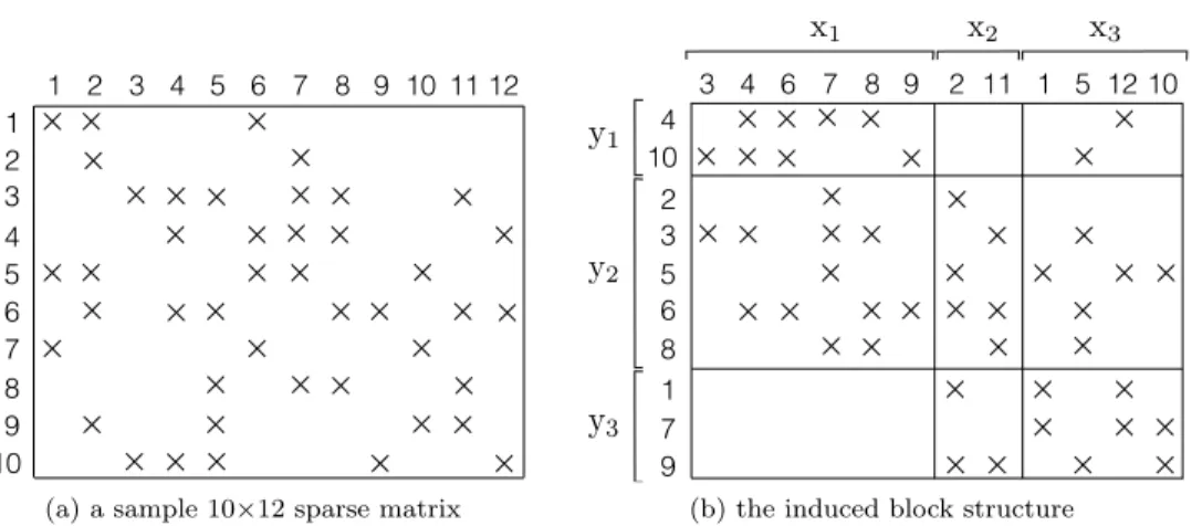
1. (expand) for each nonzero column stripe A(`)_∗k, where `6= k;

(a) form vector ˆx(k)_` which contains only those entries of x(k)_{corresponding}

to nonzero columns in A(`)_∗k and

(b) send vector ˆx(k)_` to P`,

2. for each nonzero row stripe A(k)`∗ , where `6= k; compute

(a) y_k(`)_{← A}(k)_`k x(k)and (b) y_k(`)← y(`)k + P r6=kA (k) `r xˆ (r) k

3. (fold) for each nonzero row stripe A(k)_`∗ , where `_{6= k;}

(a) form vector ˆy_k(`) which contains only those entries of y(`)k corresponding

to nonzero rows in A(k)_`∗ and

(b) send vector ˆy_k(`) to P`, 4. compute output-subvector (a) y(k) ← A(k)kkx(k), (b) y(k)_{← y}(k)_{+ A}(k) k`xˆ (`) k and (c) y(k) ← y(k)₊P `6=kˆy (k) ` .

In the well-known parallel SpMV, the messages are homogenous in the sense that

168

they pertain to either x- or y-vector entries. In the proposed row-column-parallel

169

SpMV algorithm, the number of messages are reduced with respect to the

row-column-170

parallel algorithm by making the messages heterogenous (pertaining to both x- and

171

y-vector entries), and by communicating them in a single expand-fold phase. If a

172

processor P` sends a message to processor Pk in both of the expand and fold phases,

173

then the number of messages required from P`to Pkreduces from two to one. However,

174

if a message from P` to Pk is sent only in the expand phase or only in the fold phase,

175

then there is no reduction in the number of such messages.

176

3.1. A Task categorization. We introduce a two-way categorization of

input-177

and output-vector entries and a four-way categorization of fine-grain tasks (1)

accord-178

ing to a task-and-data distribution Π(y← Ax) of matrix-vector multiply on A. For

179

a task aij, the input-vector entry xj is said to be local if both aij and xj are assigned

180

to the same processor; the output-vector entry yi is said to be local if both aij and yi

181

are assigned to the same processor. With this definition, the tasks can be classified

182

into four groups. The task

183 yi← yi+ aij× xj on Pk is          input-output-local if xj ∈ x(k) and yi∈ y(k), input-local if xj ∈ x(k) and yi6∈ y(k), output-local if xj 6∈ x(k) and yi∈ y(k), nonlocal if xj 6∈ x(k) and yi6∈ y(k). 184

Recall that an input-vector entry xj∈ x(`) is sent from P` to Pk if there exists a task

185

aij ∈ A(k)at column j, which implies that the task aij of Pk is either output-local or

186

nonlocal since xj 6∈ x(k). Similarly, for an output-vector entry yi ∈ y(`), P` receives

(7)

a partial result ˆyi from Pk if a task aij ∈ A(k), which implies that the task aij of 188

Pk is either input-local or nonlocal since yi 6∈ y(k). We can also infer from that the

189

input-output-local tasks neither depend on the input-communication phase nor incur

190

a dependency on the output-communication phase. However, the nonlocal tasks are

191

linked with both communication phases.

192

In the row-parallel algorithm, each of the fine-grain tasks is either

input-output-193

local or output-local due to the rowwise partitioning condition (6). For this reason,

194

no partial result is computed for other processors, and thus no output communication

195

is incurred. In the column-parallel algorithm, each of the fine-grain tasks is either

196

input-output-local or input-local due to the columnwise partitioning condition (7). In

197

the row-column-parallel algorithm, the input and output communications have to be

198

carried out in separate phases. The reason is that the partial results on the

output-199

vector entries to be sent are partially derived by performing nonlocal tasks that rely

200

on the input-vector entries received.

201

3.2. Local fine-grain partitioning. In order to remove the dependency

be-202

tween the two communication phases in the row-column-parallel algorithm, we

pro-203

pose the local grain partitioning where “locality” refers to the fact that each

fine-204

grain task is input-local, output-local or input-output-local. In other words, there is

205

no nonlocal fine-grain task.

206

A task-and-data distribution Π(y← Ax) of matrix-vector multiply on A is said

207

to be a local fine-grain partition if the following condition is satisfied:

208

(8) aij ∈ A(k)+ A(`) whenever yi∈ y(k) and xj∈ x(`).

209

Notice that this condition is equivalent to

210

(9) if aij ∈ A(k) then either xj∈ y(k), or yi∈ x(k), or both.

211

Due to (4) and (9), each submatrix A(k)_{becomes of the following form}

212 (10) A(k)=          0 . . . A(k)_1k . . . 0 .. . . .. ... . .. ... A(k)_k1 _{· · ·} A(k)_kk _{· · · A}(k)_kK .. . . .. ... . .. ... 0 . . . A(k)_Kk . . . 0          . 213

In this form, the tasks associated with the nonzeros of diagonal block A(k)_kk, the

off-214

diagonal blocks of the row stripe A(k)_k∗, and the off-diagonal blocks of the column-stripe

215

A(k)_∗k are input-output-local, output-local and input-local, respectively. Furthermore,

216

due to (5) and (8), each off-diagonal block Ak`of the block structure (3) induced by

217

the vector distribution (Π(x),Π(y)) becomes

218

(11) Ak`= A(k)k` + A

(`) k` , 219

and for each diagonal block we have Akk= A(k)kk.

220

In order to clarify Equations (8)–(11), we provide the following 4-way local

fine-221

grain partition on A as permuted into a 4_{×4 block structure.}

(8)

P1 P2 P3 P1 P2 P3 x1 x1 x2 x2 x3 x3 y1 y1 y2 y2 a12 a12 a13 a13 a21 a21 a22 a22 3 2 2 1 1 P1 P1 P2 P2 P3 P1 P2 P2 P3 P3 P2 P1 3 2 2 1 1 P2 P2 P3 P1 P1 P1 P3 P2 P2 P2 P3 P1 P2

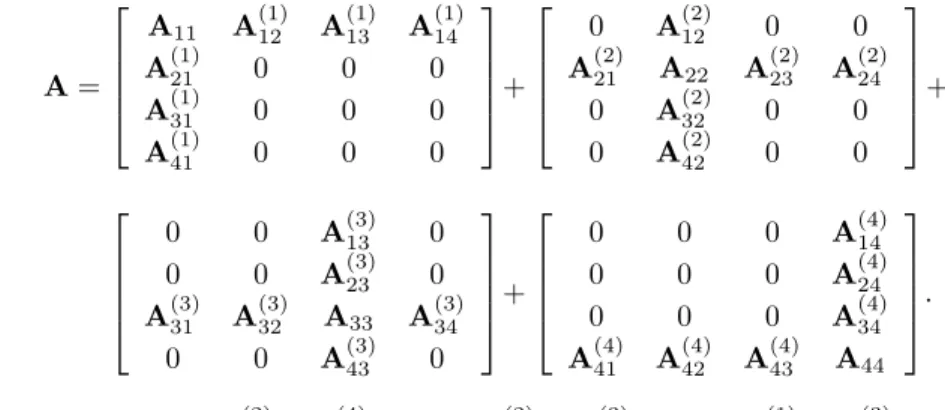
Fig. 2: A sample local fine-grain partition. Here, a12 is an output-local task, a13 is

an input-output-local task, a21is an output-local task, and a22is an input-local task.

A=      A11 A(1)12 A (1) 13 A (1) 14 A(1)₂₁ 0 0 0 A(1)₃₁ 0 0 0 A(1)₄₁ 0 0 0      +      0 A(2)₁₂ 0 0 A(2)₂₁ A22 A(2)23 A (2) 24 0 A(2)₃₂ 0 0 0 A(2)₄₂ 0 0      + 223      0 0 A(3)₁₃ 0 0 0 A(3)₂₃ 0 A(3)₃₁ A(3)₃₂ A33 A(3)34 0 0 A(3)₄₃ 0      +      0 0 0 A(4)₁₄ 0 0 0 A(4)₂₄ 0 0 0 A(4)₃₄ A(4)₄₁ A(4)₄₂ A(4)₄₃ A44      . 224 For instance, A42= A(2)42 + A (4) 42, A23= A(2)23 + A (3) 23, A31= A(1)31 + A (3) 31, . . . , etc. 225

Figure 2 displays a sample 3-way local fine-grain partition on the same sparse

226

matrix used in Figure1. In this figure, a13∈ A(1) where y1∈ y(2) and x3∈ x(1) and

227

thus a13 is an input-local task of P1. Also, a21∈ A(3) where y2∈ y(3) and x1∈ x(1)

228

and thus a21is an output-local task of P3.

229

3.3. Local row-column-parallel sparse matrix-vector multiply. As there

230

is no nonlocal tasks, the output-local tasks depend on input communication, and the

231

output communication depends on the input-local tasks. Therefore, the tasks groups

232

and communication phases can be arranged as: (i) input-local tasks; (ii)

output-233

communication, input-communication; (iii) output-local tasks and input-output-local

234

tasks. The input and output communication phases can be combined into the

expand-235

fold phase, and the output-local and input-output-local task groups can be combined

236

into a single computation phase to simplify the overall execution.

237

The local row-column-parallel algorithm is composed of three steps as shown in

238

Algorithm2. In the first step, processors concurrently perform their input-local tasks

239

which contribute to partially computed output-vector entries for other processors. In

240

the expand-fold phase, for each nonzero off-diagonal block A`k = A(k)_`k + A(`)_`k, Pk

241

prepares a message [ˆx(k)_` , ˆy(`)_k ] for P`. Here, ˆx(k)` contains the input-vector entries of 242

x(k)that are required by the output-local tasks of P`, whereas ˆy_k(`)contains the partial 243

results on the output-vector entries of y(`)_{, where the partial results are derived by}

244

performing the input-local tasks of Pk. In the last step, each processor Pk computes

245

output-subvector y(k) _{by summing the partial results computed locally by its own}

246

input-output-local tasks (step 3a) and output-local tasks (step 3b) as well as the

247

partial results received from other processors due to their input-local tasks (step 3c).

248

For a message [ˆx(k)_` , ˆy(`)_k ] from processor Pk to P`, the input-vector entries of ˆx(k)` 249

correspond to the nonzero columns of A(`)_`k, whereas the partially computed

(9)

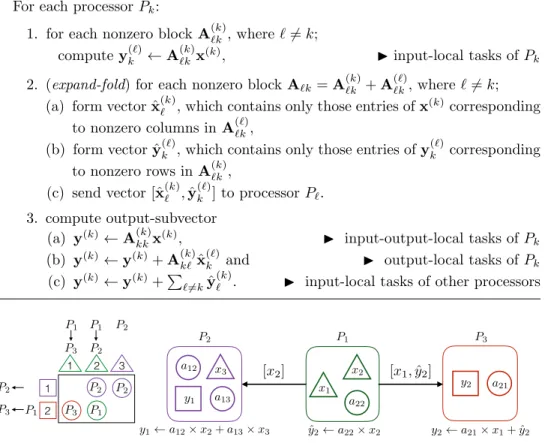
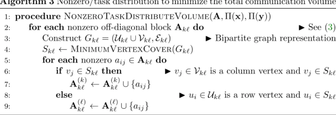
Algorithm 2The local row-column-parallel sparse matrix-vector multiply

For each processor Pk:

1. for each nonzero block A(k)_`k , where `6= k;

compute y_k(`)_{← A}(k)_`k x(k), I input-local tasks of Pk

2. (expand-fold) for each nonzero block A`k= A(k)`k + A

(`)

`k, where `6= k;

(a) form vector ˆx(k)_` , which contains only those entries of x(k)_{corresponding}

to nonzero columns in A(`)`k,

(b) form vector ˆy(`)_k , which contains only those entries of y(`)_k corresponding to nonzero rows in A(k)_`k,

(c) send vector [ˆx(k)_` , ˆy_k(`)] to processor P`.

3. compute output-subvector (a) y(k)_{← A}(k) kkx(k), I input-output-local tasks of Pk (b) y(k) ← y(k)_{+ A}(k) k`xˆ (`)

k and I output-local tasks of Pk

(c) y(k)

← y(k)₊P

`6=kˆy (k)

` . I input-local tasks of other processors

aij P` Pk xj yi xj yˆi ˆ yi ˆyi+ aij⇥ xj yi yi+ ˆyi P` Pk P` Pk aij aij xj xj yi yi ˆ yi xj ˆ yi ˆyi+ aij⇥ xj yi yi+ ˆyi yi yi+ aij⇥ xj ˆ y2 a22⇥ x2 y1 a12⇥ x2+ a13⇥ x3 y2 a21⇥ x1+ ˆy2 P1 P2 P3 x1 x2 x3 y1 y2 a12 a13 _a₂₂ a21 [x2] [x1, ˆy2] Pr 3 2 2 1 1 P1 P1 P2 P2 P3 P1 P2 P2 P3 P3 P2 P1

Fig. 3: An illustration of Algorithm2 for the local fine-grain partition in Figure2.

vector entries of ˆy_k(`) correspond to the nonzero rows of A(k)_`k . That is, ˆx(k)_` = [xj : 251

aij ∈ A(`)`k] and ˆy (`)

k = [ˆyi : aij ∈ A(k)`k]. This message is heterogeneous if A

(k) `k and 252

A(`)_`k are both nonzero and homogeneous otherwise. We also note that the number of

253

messages is equal to the number of nonzero off-diagonal blocks of the block structure

254

(3) of A induced by the vector distribution (Π(x), Π(y)). Figure 3 illustrates the

255

steps of Algorithm 2 on the sample local fine-grain partition given in Figure2. As

256

seen in the figure, there are only two messages to be communicated. One message

257

is homogeneous, which is from P1 to P2 and contains only an input-vector entry x2,

258

whereas the other message is heterogeneous, which is from P1 to P3 and contains an

259

input-vector entry x1 and a partially computed output-vector entry ˆy2.

260

4. Two proposed methods for local row-column-parallel partitioning.

261

We propose two methods to find a local row-column-parallel partition that is required

262

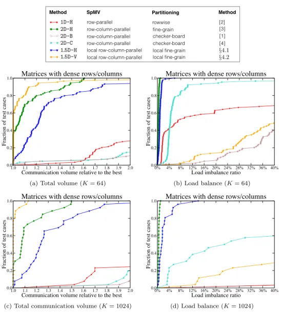
for 1.5D local row-column-parallel SpMV. One method finds vector and nonzero

dis-263

tributions simultaneously, whereas the other one has two parts in which vector and

264

nonzero distributions are found separately.

265

4.1. A directed hypergraph model for simultaneous vector and nonzero

266

distribution. In this method, we adopt the elementary hypergraph model for the

267

fine-grain partitioning [16] and introduce an additional locality constraint on

par-268

titioning in order to obtain a local fine-grain partition. In this hypergraph model

(10)

H2D= (V, N ), there is an input-data vertex for each input-vector entry, an output-270

data vertex for each output-vector entry and a task vertex for each fine-grain task (or

271

per matrix nonzero) for a given matrix A. That is,

272

V = {vx(j) : xj∈ x} ∪ {vy(i) : yi∈ y} ∪ {vz(ij) : aij ∈ A} . 273

The input- and output-data vertices have zero weights, whereas the task vertices have

274

unit weights. In_H2D, there is an input-data net for each input-vector entry, and an

275

output-data net for each output-vector entry. An input-data net nx(j), corresponding

276

to the input-vector entry xj, connects all task vertices associated with the nonzeros at

277

column j as well as the input-data vertex vx(j). Similarly, an output-data net ny(i),

278

corresponding to the output-vector entry yi, connects all task vertices associated with

279

the nonzeros at row i as well as the output-data vertex vy(i). That is

280

N = {nx(j) : xj ∈ x} ∪ {ny(i) : yi∈ y} , 281

nx(j) ={vx(j)} ∪ {vz(ij) : aij ∈ A, 1 ≤ i ≤ m} , and 282

ny(i) ={vy(i)} ∪ {vz(ij) : aij ∈ A, 1 ≤ j ≤ n}. 283

Note that each input-data net connects a separate input-data vertex, whereas

284

each output-data net connects a separate output-data vertex. We associate nets with

285

their respective data vertices.

286

We enhance the elementary row-column-net hypergraph model by imposing

di-287

rections on the nets; this is required for modeling the dependencies and their nature.

288

Each input-data net nx(j) is directed from the input-data vertex vx(j) to the task

289

vertices connected by nx(j), and each output-data net ny(i) is directed from the task

290

vertices connected by ny(i) to the output-data vertex vy(i). Each task vertex vz(ij)

291

is connected by a single input-data-net nx(j) and a single output-data-net ny(i).

292

In order to impose the locality in the partitioning, we introduce the following

293

constraint for vertex partitioning on the directed hypergraph model _H2D: each task

294

vertex vz(ij) should be assigned to the part that contains either input-data vertex

295

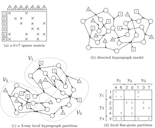
vx(j), or output-data vertex vy(i), or both. Figure 4adisplays a sample 6×7 sparse

296

matrix. Figure 4b illustrates the associated directed hypergraph model. Figure 4c

297

shows a 3-way vertex partition of this directed hypergraph model satisfying the locality

298

constraint, and Fig.4dshows the local fine-grain partition decoded by this partition.

299

Instead of developing a partitioner for this particular directed hypergraph model,

300

we propose a task-vertex amalgamation procedure which will help in meeting the

301

described locality constraint by using a standard hypergraph partitioning tool. For

302

this, we adopt and adapt a simple-yet-effective approach of Pelt and Bisseling [15]. In

303

our adaptation, we amalgamate each task vertex vz(ij) into either input-data vertex

304

vx(j) or output-data vertex vy(i) according to the number of task vertices connected

305

by nx(j) and ny(i), respectively. That is, vz(ij) is amalgamated into vx(j) if column j

306

has a smaller number of nonzeros than row i, and otherwise it is amalgamated into

307

vy(i), where the ties are broken arbitrarily. The result is a reduced hypergraph that

308

contains only the input- and output-data vertices amalgamated with the task vertices

309

where the weight of a data vertex is equal to the number of task vertices amalgamated

310

into that data vertex. As a result, the locality constraint on vertex partitioning of the

311

initial directed hypergraph naturally holds on any vertex partitioning on the reduced

312

hypergraph. It so happens that after this process, the net directions become irrelevant

313

for partitioning, and hence one can use the standard hypergraph partitioning tools.

314

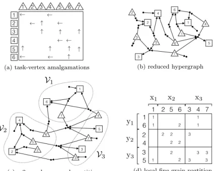
Figure5illustrates how to obtain a local fine-grain partition through the described

315

(d) local fine-grain partition

Fig. 4: An illustration of attaining a local fine-grain partition through vertex par-titioning of the directed hypergraph model that satisfies locality constraints. The input- and output-data vertices are drawn with triangles and rectangles, respectively.

a task vertex vz(ij) is amalgamated into input-data vertex vx(j) and output-data

317

vertex vy(i), respectively. The reduced hypergraph obtained by these task-vertex

318

amalgamations is shown in Figure5b. Figures5cand5dshow a 3-way vertex partition

319

of this reduced hypergraph and the obtained local fine-grain partition, respectively. As

320

seen in these figures, task a35is assigned to processor P2since vz(3, 5) is amalgamated

321

into vx(5), and vx(5) is assigned to V2. 322

We emphasize here that the reduced hypergraph constructed as above is

equiv-323

alent to the hypergraph model of Pelt and Bisseling [15]. In that original work, the

324

use of this model was only for two-way partitioning (of the fine grain model) which is

325

then used for K-way fine-grain partitioning recursively. But this distorts the locality

326

of task vertices so that a partition obtained in further recursive steps is no more a

327

local fine-grain partition. That is why the adaptation was necessary.

328

4.2. Nonzero distribution to minimize the total communication

vol-329

ume. This method is composed of two parts. The first parts finds a vector

distri-330

bution (Π(x), Π(y)). The second part finds a nonzero/task distribution Π(A) that

331

exactly minimizes the total communication volume over all possible local fine-grain

332

partitions which abide by (Π(x), Π(y)) of the first part. The first part can be

ac-333

complished by any conventional data partitioning method such as 1D partitioning.

334

Therefore, this section is devoted to the second part.

335

Consider the block structure (3) of A induced by (Π(x), Π(y)). Recall that in

336

a local fine-grain partition, due (11), the nonzero/task distribution is such that each

(12)

3 (c) a 3-way hypergraph partition

diagonal block Akk = A(k)kk, and each off-diagonal block Ak` is a nonzero-disjoint

338

summation of the form Ak` = A(k)k` + A

(`)

k`. This corresponds to assigning each

339

nonzero of Akkto Pk, for each diagonal block Akk, and assigning each nonzero of Ak`

340

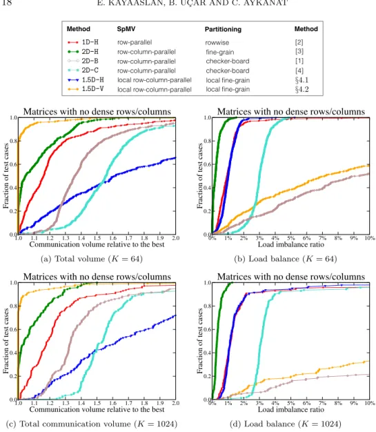
to either Pk or P`. Figure6 illustrates a sample 10×12 sparse matrix and its block

341

structure induced by a sample 3-way vector distribution which incurs four messages:

342

from P3 to P1, from P1 to P2, from P3 to P2, and from P2 to P3 due to A13, A21,

343

A23 and A32, respectively.

344

Since diagonal blocks and zero off-diagonal blocks do not incur any

communica-345

tion, we focus on the nonzero off-diagonal blocks. Consider a nonzero off-diagonal

346

block Ak` which incurs a message from P` to Pk. The volume of this message is

347

determined by the distribution of tasks of Ak`between Pk and P`. This in turn

im-348

plies that distributing the tasks of each nonzero off-diagonal block can be performed

349

independently for minimizing the total communication volume.

350

In the local row-column-parallel algorithm, P` sends [ˆx(k)` , ˆy (`)

k ] to Pk. Here, ˆx(k)` 351

corresponds to the nonzero columns of A(`)_`k, and ˆy(`)_k corresponds to the nonzero rows

352

of A(k)_`k , for a nonzero/task distribution Ak`= A(k)_k` + A(`)_k`. Then, we can derive the 353

following formula for the communication volume φk`from P` to Pk:

354

(12) φk`= ˆn(A(k)k`) + ˆm(A

(`) k`), 355

where ˆn(_{·) and ˆ}m(_{·) refer to the number of nonzero columns and nonzero rows of the}

356

input submatrix, respectively. The total communication volume φ is then computed

357

by summing the communication volumes incurred by each nonzero off-diagonal block

358

of the block structure. Then, the problem of our interest can be described as follows.

359 360

(13)

Fig. 6: A sample 10_{×12 sparse matrix A and its block structure induced by}

input-data distribution Π(x) = _{x(1)_{, x}(2)_{, x}(3)

} and output-data distribution Π(y) = {y(1)_{, y}(2)_{, y}(3)

}, where x(1) ₌

{x3, x4, x6, x7, x8, x9}, x(2) = {x2, x11}, x(3) =

{x1, x5, x12, x10}, y(1)={y4, y10}, y(2)={y2, y3, y5, y6, y8}, and y(3) ={y1, y7, y9}.

Problem 1. Given A and a vector distribution (Π(x), Π(y)), find a nonzero/task

361

distribution Π(A) such that (i) each nonzero off-diagonal block has the form Ak` =

362

A(k)_k` + A(`)_k`; (ii) each diagonal block Akk = A(k)kk in the block structure induced by 363

(Π(x), Π(y)); and (iii) the total communication volume φ =P

k6=`φk` is minimized.

364

Let Gk`= (Uk`∪ Vk`, Ek`) be the bipartite graph representation of Ak`, where

365

Uk` and Vk` are the set of vertices corresponding to the rows and columns of Ak`,

366

respectively, and_Ek` is the set of edges corresponding to the nonzeros of Ak`. Based

367

on this notation, the following theorem states a correspondence between the problem

368

of distributing nonzeros/tasks of Ak`to minimize the communication volume φk`from

369

P` to Pk and the problem of finding a minimum vertex cover of Gk`. Before stating

370

the theorem we give a brief definition of vertex covers for the sake of completeness.

371

A subset of vertices of a graph is called vertex cover if each of the graph edges is

372

incident to any of the vertices in this subset. A vertex cover is minimum if its size

373

is the least possible. In bipartite graphs, the problem of finding a minimum vertex

374

cover is equivalent to the problem of finding a maximum matching [13]. Aschraft and

375

Liu [1] describe a similar application of vertex covers.

376

Theorem 1. Let Ak` be a nonzero off-diagonal block andGk`= (Uk`∪ Vk`,Ek`)

377

be its bipartite graph representation.

378

1. For any vertex cover Sk`ofGk`, there is a nonzero distribution Ak`= A(k)k` +

379

A(`)_k` such that _|Sk`| ≥ ˆn(A(k)k`) + ˆm(A (`) k`), 380

2. For any nonzero distribution Ak`= A(k)k` + A

(`)

k`, there is a vertex coverSk`

381

of Gk` such that |Sk`| = ˆn(A(k)k`) + ˆm(A (`) k`). 382

Proof. We prove the two parts of the theorem separately.

383

1) Take any vertex cover Sk` of Gk`. Consider any nonzero distribution Ak` =

(14)

A(k)_k` + A(`)_k` such that 385 (13) aij∈      A(k)_k` if vj∈ Sk` and ui6∈ Sk`, A(`)_k` if vj6∈ Sk` and ui∈ Sk`, A(k)_k` or A(`)k` if vj∈ S` and ui∈ Sk`. 386

Since vj ∈ Sk` for every aij ∈ A(k)k` and ui ∈ Sk` for every aij ∈ A(`)k`, |Sk`∩ Vk`| ≥ 387

ˆ

n(A(k)k`) and|Sk`∩ Uk`| ≥ ˆm(A(`)k`), which in turn leads to 388

(14) _|Sk`| ≥ ˆn(A(k)k`) + ˆm(A

(`) k`). 389

2) Take any nonzero distribution Ak`= A(k)k` + A

(`)

k`. Consider Sk`={ui∈ Uk`:

390

aij ∈ A(`)k`} ∪ {vj ∈ Vk`: aij ∈ A(k)k`} where |Sk`| = ˆn(A(k)k`) + ˆm(A (`)

k`). Now, consider

391

a nonzero aij ∈ Ak` and its corresponding edge {ui, vj} ∈ Ek`. If aij ∈ A(k)_k`, then 392

vj ∈ Sk`. Otherwise, ui∈ Sk`since aij∈ A(`)k`. So, Sk`is a vertex cover of Gk`. 393

At this point, however, it is still not clear how the reduction from the problem

394

of distributing the nonzeros/tasks to the problem of finding the minimum vertex

395

cover holds. For this purpose, using Theorem 1, we show that a minimum vertex

396

cover of Gk` can be decoded as a nonzero distribution of Ak` with the minimum

397

communication volume φk`as follows. Let S∗k`be a minimum vertex cover of Gk`and

398

φ∗

k`be the minimum communication volume incurred by a nonzero/task distribution

399

of Ak`. Then,|Sk`∗| = φ∗k`, since the first and second parts of Theorem1imply|Sk`∗ | ≥ 400

φ∗

k` and |S∗k`| ≤ φ∗k`, respectively. We decode an optimal nonzero/task distribution

401

Ak`= A(k)k` + A (`)

k` out of Sk`∗ according to (13) where one such distribution is

402 (15) A(k)_k` ={aij ∈ Ak`: vj∈ S∗k`} and A (`) k` ={aij ∈ Ak`: vj6∈ S ∗ k`}. 403

Let φk` be the communication volume incurred by this nonzero/task distribution.

404

Then,_|S∗

k`| ≥ φk`due to (14), and φk`= φ∗k` since φk`∗ =|Sk`∗| ≥ φk`≥ φ∗k`. 405

Figure 7 illustrates the reduction on a sample 5_{×6 nonzero off-diagonal block}

406

Ak`. The left side and middle of this figure respectively display Ak`and its bipartite

407

graph representation Gk`, which contains 5 row vertices and 6 column vertices. On

408

the middle of the figure, a minimum vertex cover Sk`that contains two row vertices

409

{u3, u6} and two column vertices {v7, v8} is also shown. The right side of the figure

410

displays how this minimum vertex cover is decoded as a nonzero/task distribution

411

Ak` = A(k)_k` + A(`)_k`. As a result of this decoding, P` sends [x7, x8, ˆy3, ˆy6] to Pk in a 412

single message. Note that a nonzero corresponding to an edge connecting two cover

413

vertices can be assigned to either A(k)_k` or A(`)_k` without changing the communication

414

volume from P` to Pk. The only change that may occur is in the values of partially

415

computed output-vector entries to be communicated. For instance, in the figure,

416

nonzero a37is assigned to A(k)_k`. Since both u3and v7 are cover vertices, a37 could be

417

assigned to A(`)_k` with no change in the communicated entries but the value of ˆy3.

418

Algorithm3gives a sketch of our method to find a nonzero/task distribution that

419

minimizes the total communication volume based on Theorem1. For each nonzero

off-420

diagonal block Ak`, the algorithm first constructs Gk`, then obtains a minimum vertex

421

cover Sk`, and then decodes Sk` as a nonzero/task distribution Ak` = A(k)k` + A

(`) k` 422

according to (15). Hence, the communication volume incurred by Ak`is equal to the

423

size of the cover _|Sk`|. In detail, each row vertex ui on the cover incurs an output

(15)

u2 u3 u5 u8 v3 v4 v6 v7 v8 v9 u6 Sk`={u3, u6, v7, v8} Gk` Ak` 2 3 5 6 8 3 4 6 7 8 9 yk={y2, y3, y5, y6, y8} x`={x3, x4, x6, x7, x8, x9} 2 3 5 6 8 3 4 6 7 8 9 A(`)k` Output-communication [ˆy3, ˆy6] A(k)k` 2 3 5 6 8 3 4 6 7 8 9 Input-communication [x7, x8]

Fig. 7: The minimum vertex cover model for minimizing the communication volume φk`from P` to Pk. According to the vertex cover Sk`, P` sends [x7, x8, ˆy3, ˆy6] to Pk.

communication of ˆyi∈ ˆy(k)` , and each column vertex vj on the cover incurs an input

425

communication of xj ∈ ˆx(`)k . We recall that P` sends ˆy(k)` and ˆx (`)

k to Pk in a single

426

message in the proposed row-column-parallel sparse matrix-vector multiply algorithm.

427

Algorithm 3Nonzero/task distribution to minimize the total communication volume

1: procedure NonzeroTaskDistributeVolume(A, Π(x), Π(y))

2: for eachnonzero off-diagonal block Ak`do I See (3)

3: Construct Gk`= (Uk`∪ Vk`,Ek`) I Bipartite graph representation

4: Sk` ← MinimumVertexCover(Gk`)

5: for eachnonzero aij∈ Ak` do

6: if vj∈ Sk` then I vj∈ Vk`is a column vertex and vj ∈ Sk`

7: A(k)_k` _{← A}(k)_k` _{∪ {a}ij}

8: else I ui∈ Uk` is a row vertex and ui∈ Sk`

9: A(`)_k` _{← A}(`)_k` _{∪ {a}ij}

Figure 8 illustrates the steps of Algorithm 3 on the block structure given in

428

Figure 6b. Figure 8a shows four bipartite graphs each corresponding to a nonzero

429

off-diagonal block. In this figure, a minimum vertex cover for each bipartite graph

430

is also shown. Figure 8b illustrates how to decode a local fine-grain partition from

431

those minimum vertex covers. In this figure, the nonzeros are represented with the

432

processor to which they are assigned. As seen in the figure, the number of entries sent

433

from P1to P2is four, that is, φ21= 4, and the number of entries sent from P3 to P1,

434

from P3 to P2 and from P2 to P3are all two, that is, φ13= φ23= φ32= 2.

435

We note here that the objective of this method is to minimize the total

com-436

munication volume under a given vector distribution. Since blocks of nonzeros are

437

assigned, a strict load balance cannot be always maintained.

438

5. Related work. Here we review recent related work on matrix partitioning

439

for parallel SpMV.

440

Kuhlemann and Vassilevski [14] recognize the need to reduce the number of

mes-441

sages in parallel sparse matrix vector multiply operations with matrices corresponding

(16)

1.5D PARALLEL SPARSE MATRIX-VECTOR MULTIPLY 15 u2 u3 u5 u8 v3 v4 v6 v7 v8 v9 u6 G21 G13 v12 v5 u4 u10 G32 v2 v11 u1 u9 G23 v5 v1 v10 v12 u3 u5 u6 u8 S21={v7, v8, u3, u6} S23={v5, u5} S13={v12, u10} S32={v2, u9}

(a) a minimum vertex cover for each nonzero off-diagonal block of Figure6b.

Fig. 8: An optimal nonzero distribution minimizing the total communication volume

obtained by Algorithm 3. The matrix nonzeros are represented with the

proces-sors they are assigned to. The total communication volume is 10, where P1 sends

[x7, x8, ˆy3, ˆy6] to P2; P3 sends [x12, ˆy10] to P1; P3 sends [x2, ˆy9] to P1; and P3 sends

[x5, ˆy5] to P2.

to scale-free graphs. They present methods to embed the given graph in a bigger one

443

to reduce the number of messages. The gist of the method is to split a vertex into

444

a number of copies (the number is determined with a simple calculation to limit the

445

maximum number of messages per processor). In such a setting, the SpMV

opera-446

tions with the matrix associated with the original graph, y←Ax, is then cast as triple

447

sparse matrix vector products of the form y_{← Q}T_{(B(Qx)). This original work can}

448

be extended to other matrices (not necessarily symmetric, nor square) by recognizing

449

the triplet product as a communication on x for duplication (for the columns that

450

are split), communication of x vector entries (duplicates are associated with different

451

destinations), multiplication, and as a communication on the output vector (for the

452

rows that are split) to gather results. This exciting extension requires further analysis.

453

Boman et al. [2] propose a 2D partitioning method obtained by post-processing

454

a 1D partition. Given a 1D partition among P processors, the method maps the

455

P_{× P block structure to a virtual mesh of size P}r× Pcand reassigns the off-diagonal

456

blocks so as to limit the number of messages per processor by Pr+ Pc. The

post-457

processing is fast, and hence the method is as nearly efficient as a 1D partitioning

458

method. However, the communication volume and the computational load balance

459

obtained in the 1D partitioning phase are disturbed and the method does not have

460

any means to control the perturbation. The proposed two-part method (Section4.2),

461

is similar to this work in this aspect; a strict balance cannot always be achieved; yet

462

a finer approach is discussed in the preliminary version of the paper [12].

463

Pelt and Bisseling [15] propose a model to partition sparse matrices into two

464

parts (which then can be used recursively to partition into any number of parts). The

465

essential idea has two steps. First, the nonzeros of a given matrix A are split into

466

two different matrices (of the same size as the original matrix), say A = Ar+ Ac.

467

Second, Ar and Ac are partitioned together, where Ar is partitioned rowwise, and

468

Ac is partitioned columnwise. As all nonzeros of A are in only one of Ar or Ac, the

469

final result is a two-way partitioning of the nonzeros of A. The resulting partition on

(17)

Aachieves load balance and reduces the total communication volume by the standard

471

hypergraph partitioning techniques.

472

Two-dimensional partitioning methods that bound the maximum number of

mes-473

sages per processor, such as the checkerboard [5, 8] and orthogonal recursive

bisec-474

tion [17] based methods, have been used in modern applications [18,20], sometimes

475

without graph/hypergraph partitioning [19]. In almost all cases, inadequacy of 1D

476

partitioning schemes are confirmed.

477

All previous work (including those that were summarized above) assumes the

478

standard SpMV algorithm based on expanding x-vector entries, performing multiplies

479

with matrix entries, and folding y-vector entries. Compared to all these previous work,

480

ours has therefore a distinctive characteristic. In this work, we introduce the novel

481

concept of heterogeneous messages where x-vector and partially computed y-vector

482

entries are possibly communicated within the same message packet. In order to make

483

use of this, we search for a special 2D partition on the matrix nonzeros in which a

484

nonzero is assigned to a processor holding either the associated input-vector entry, or

485

the associated output-vector entry, or both. The implication is that the proposed local

486

row-column-parallel SpMV algorithm requires only a single communication phase (all

487

the previous algorithms based on 2D partitions require two communication phases)

488

as is the case for the parallel algorithms based on 1D partitions; yet the proposed

489

algorithm achieves a greater flexibility to reduce the communication volume than the

490

1D methods.

491

6. Experiments. We performed our experiments on a large selection of sparse

492

matrices obtained from the University of Florida (UFL) sparse matrix collection [9].

493

We used square and structurally symmetric matrices with 500–10M nonzeros. At the

494

time of experiments, we had 904 such matrices. We discarded 14 matrices as they

495

contain diagonal entries only, and we also excluded one matrix (kron g500-logn16)

496

because it took extremely long to have a partition with the hypergraph partitioning

497

tool used in the experiments. We conducted our experiments for K = 64 and K =

498

1024 and omit the cases when the number of rows is less than 50_{× K. As a result, we}

499

had 566 and 168 matrices for the experiments with K = 64 and 1024, respectively.

500

We separate all our test matrices into two groups according to the maximum number

501

of nonzeros per row/column, more precisely, according to whether the test matrix

502

contains a dense row/column or not. We say a row/column dense if it contains at

503

least 10√m nonzeros, where m denotes the number of rows/columns. Hence, for

504

K = 64 and 1024, the first group respectively contains 477 and 142 matrices that

505

have no dense rows/columns out of 566 and 168 test matrices. The second group

506

contains the remaining 89 and 26 matrices, each having some dense rows/column, for

507

K = 64 and 1024, respectively.

508

In the experiments, we evaluated the partitioning qualities of the local fine-grain

509

partitioning methods proposed in Section 4 against 1D rowwise (1D-H [3]), the 2D

510

fine-grain (2D-H [4]), and two checkerboard partitioning methods (2D-B [2], 2D-C [5]).

511

For the method proposed in Section4.1, we obtain a local fine-grain partition through

512

the directed hypergraph model (1.5D-H) using the procedure described at the end of

513

that subsection. For the method proposed in Section4.2(1.5D-V), the required vector

514

distribution is obtained by 1D rowwise partitioning using the column-net hypergraph

515

model. Then, we obtain a local fine-grain partition on this vector distribution with a

516

nonzero/task distribution that minimizes the total communication volume.

517

The 1D-H, 2D-H, 2D-C and 1.5D-H methods are based on hypergraph models.

Al-518

though all these models allow arbitrary distribution of the input- and output-vectors,

(18)

in the experiments, we consider conformal partitioning of input and output vectors,

520

by using vertex amalgamation of the input- and output-vector entries [16]. We used

521

PaToH [3,6] with default parameters where the maximum allowable imbalance ratio

522

is 3% for partitioning. We also notice that the 1.5D-V and 2D-B methods are based

523

on 1D-H and keeps the vector distribution obtained from 1D-H intact. Hence, in the

524

experiments, the input and output vectors for those methods are conformal as well.

525

Finally, since PaToH depends on randomization, we report the geometric mean of ten

526

different runs for each partitioning instance.

527

In all experiments, we report the results using performance profiles [10] which is

528

very helpful in comparing multiple methods over a large collection of test cases. In a

529

performance profile, we compare methods according to the best performing method

530

for each test case and measure in what fraction of the test cases a method performs

531

within a factor of the best observed performance. For example, a point (abscissa =

532

1.05, ordinate = 0.30) on the performance curve of a given method refers to the fact

533

that for 30% of the test cases, the method performs within a factor of 1.05 of the best

534

observed performance. As a result, a method that is closer to top-left corner is better.

535

In the load balancing performance profiles displayed in Figures9b,9d, 10b and10d,

536

we compare performance results with respect to the performance of perfect balance

537

instead best observed performance. That is, a point (abscissa = 6% and ordinate =

538

0.40) on the performance curve of a given method means that for 40% of the test

539

cases, the method produces a load imbalance ratio less than or equal to 6%.

540

Figures 9 and10 both display performance profiles of four task-and-data

distri-541

bution methodsin terms of the total communication volume and the computational

542

load imbalance. Figure 9 displays performance profiles for the set of matrices with

543

no dense rows/columns, whereas Figure10 displays performance profiles for the set

544

of matrices containing dense rows/columns.

545

As seen in Figure 9, for the set of matrices with no dense rows/columns, the

546

relative performances of all methods are similar for K = 64 and K = 1024 in terms

547

of both communication volume and load imbalance. As seen in Figures 9a and 9c,

548

all methods except the 1.5D-H method achieve a total communication volume at most

549

30% more than the best in almost 80% of the cases in this set of matrices. As seen

550

in these two figures, the proposed 1.5D-V method performs significantly better than

551

all other methods, whereas the 2D-H method is the second best performing method.

552

As also seen in the figures, 1D-H displays the third best performance, whereas 1.5D-H

553

shows the worst performance. As seen in Figures9band9d, in terms of load balance,

554

the 2D-H method is the best performing method. As also seen in the figures, the

555

proposed 1.5D-V method displays considerably worse performance than the others.

556

Specifically, all methods except 1.5D-V achieve a load imbalance below 3% in almost all

557

test cases. In terms of the total communication volume, 2D checkerboard partitioning

558

methods perform considerably worse than 1.5D-V, 2D-H and 1D-H methods. The first

559

alternative 2D-B obtains better results than 2D-C. For load balance, 2D-C behaves

560

similar to 1D-H, 2D-H and 1.5D-H methods except that 2D-C achieves a load imbalance

561

below 5% (instead of 3%) for almost all instances. 2D-B behaves similar to 1.5D-V,

562

and does not achieve a good load balance.

563

As seen in Figure10, for the set of matrices with some dense rows/columns, all

564

methods display a similar performance for K = 64 and K = 1024 in terms of the

565

total communication volume. As in the previous dataset, in terms of the total

com-566

munication volume, the 1.5D-V and 2D-H methods are again the best and second best

567

methods, respectively, as seen in Figures10a and 10c. As also seen in these figures,

568

1.5D-His the third best performing method in terms of the total communication

(19)

SpMV Partitioning Method Method

1.0 1.5 2.0 2.5 3.0 3.5 4.0

Partitioning time relative to the best 0.0 0.2 0.4 0.6 0.8 1.0

Fraction of test cases

1D 2D 1.5D 1.5D-V 1.5D-L

Matrices with or without dense rows (K = 1024)

local row-column-parallel local fine-grain

1.5D-H §4.1

1.0 1.5 2.0 2.5 3.0 3.5 4.0

1D 2D 1.5D 1.5D-V 1.5D-L

local row-column-parallel

1.5D-V local fine-grain §4.2

1.0 1.5 2.0 2.5 3.0 3.5 4.0

1D 2D 1.5D 1.5D-V 1.5D-L

row-parallel rowwise [2]

1.0 1.5 2.0 2.5 3.0 3.5 4.0

Partitioning time relative to the best

0.0 0.2 0.4 0.6 0.8 1.0

1D 2D 1.5D 1.5D-V 1.5D-L Matrices with or without dense rows (K = 1024)

row-column-parallel fine-grain [3] row-column-parallel checker-board [4] row-column-parallel checker-board [1] 1D-H 2D-H 2D-B 2D-C 1.0 1.1 1.2 1.3 1.4 1.5 1.6 1.7 1.8 1.9 2.0

Communication volume relative to the best

0.0 0.2 0.4 0.6 0.8 1.0

Matrices with no dense rows/columns

(a) Total volume (K = 64)

0% 1% 2% 3% 4% 5% 6% 7% 8% 9% 10%

Load imbalance ratio

0.0 0.2 0.4 0.6 0.8 1.0

(b) Load balance (K = 64)

1.0 1.1 1.2 1.3 1.4 1.5 1.6 1.7 1.8 1.9 2.0

0.0 0.2 0.4 0.6 0.8 1.0

(c) Total communication volume (K = 1024)

0% 1% 2% 3% 4% 5% 6% 7% 8% 9% 10%

0.0 0.2 0.4 0.6 0.8 1.0

(d) Load balance (K = 1024)

Fig. 9: Performance profiles comparing the total communication volume and load balance using test matrices with no dense rows/columns for K = 64 and 1024. ume, whereas 1D-H shows considerably worse performance. The 2D-H method achieves

570

near-to-perfect load balance in almost all cases, as seen in Figures 10band 10d. As

571

also seen in these figures, the 1.5D-H method displays a load imbalance lower than

ap-572

proximately 6% and 14% for all test matrices for K = 64 and 1024, respectively. This

573

shows the success of the vertex amalgamation procedure within the context of the

574

directed hypergraph model described in Section4.1. As seen in Figure10c, the total

575

communication volume does not exceed the best method by 40% in about 75% and

576

85% of the test cases for the 1.5D-H and 2D-H methods, respectively, for K = 1024.

577

The two 2D checkerboard methods display considerably worse performance than the

578

others (except 1D-H, which also shows a poor performance) in terms of the total

com-579

munication volume. When K = 64, 2D-C shows an acceptable performance however

580

when K = 1024 its performance considerably deteriorates in terms of load balance.

581

2D-B obtains worse results. This not surprising since 2D-B is a modification of 1D-H

(20)

SpMV Partitioning Method Method

1.0 1.5 2.0 2.5 3.0 3.5 4.0

1D 2D 1.5D 1.5D-V 1.5D-L

local row-column-parallel local fine-grain

1.5D-H §4.1

1.0 1.5 2.0 2.5 3.0 3.5 4.0

1D 2D 1.5D 1.5D-V 1.5D-L

local row-column-parallel

1.5D-V local fine-grain §4.2

1.0 1.5 2.0 2.5 3.0 3.5 4.0

1D 2D 1.5D 1.5D-V 1.5D-L

row-parallel rowwise [2]

1.0 1.5 2.0 2.5 3.0 3.5 4.0

Partitioning time relative to the best

0.0 0.2 0.4 0.6 0.8 1.0

1D 2D 1.5D 1.5D-V 1.5D-L Matrices with or without dense rows (K = 1024)

row-column-parallel fine-grain [3] row-column-parallel checker-board [4] row-column-parallel checker-board [1] 1D-H 2D-H 2D-B 2D-C 1.0 1.1 1.2 1.3 1.4 1.5 1.6 1.7 1.8 1.9 2.0

0.0 0.2 0.4 0.6 0.8 1.0

Matrices with dense rows/columns

(a) Total volume (K = 64)

0% 4% 8% 12% 16% 20% 24% 28% 32% 36% 40%

0.0 0.2 0.4 0.6 0.8 1.0

(b) Load balance (K = 64)

1.0 1.1 1.2 1.3 1.4 1.5 1.6 1.7 1.8 1.9 2.0

0.0 0.2 0.4 0.6 0.8 1.0

(c) Total communication volume (K = 1024)

0% 4% 8% 12% 16% 20% 24% 28% 32% 36% 40%

0.0 0.2 0.4 0.6 0.8 1.0

(d) Load balance (K = 1024)

Fig. 10: Performance profiles comparing the total communication volume and the load balance on test matrices with dense rows/columns for K = 64 and 1024.

whose load balance performance is already very poor.

583

Figures 11a and 11b compare the methods in terms of the total and maximum

584

message counts, respectively, using all test matrices for K = 1024. We note that

585

these are secondary metrics and none of the methods addresses them explicitly as the

586

main objective function. Since 1.5D-V uses the conformal distribution of the

input-587

and output-vectors obtained from 1D-H, the total and the maximum message count

588