Digital Plasma Control System and Alcasim Simulation Code
for Alcator C-Mod
by
Marco Ferrara
Laurea in Ingegneria Elettronica, UniversitA di L'Aquila (2001)
r
w
Submitted to the Department of Nuclear Science and Engineering
in partial fulfillment of the requirements for the degree of
m
Master of Science
C-at the
MASSACHUSETTS INSTITUTE OF TECHNOLOGY
September 2005
() Massachusetts Institute of Technology 2005
The author hereby grants to Massachusetts Institute of Technology permission to
reproduce and
to distribute copies of this thesis document in whole or in part.
Signature
of
Author...
.
...
.
..
...
Department of Nuclear Science and Engineering
August 19, 2005
Certified
by
...
.
... '.
...
Ian H. Hutchinson
Chair and Professor, Department of Nuclear Science and Engineering
Thesis Supervisor
Certified
by ...
/ ...
Stephen M. Wolfe
Principal Research Scientist, Alcator Project
E
-
I
~ Thesis
Supervisor
Accepted
by
... ...
.. ... .
-M 0 01 C OE
8
6 r 300N>o
9
C" K w1"Chfts
Contents
I DPCS Digital Plasma Control System
1 Introduction
2 Implementation of Hybrid
3 Implementation of DPCS3.1 Benchmarking and debugging DPCS ... 3.2 DPCS real time code and time performance ...
II
Alcasim simulation code for Alcator C-Mod
4 Introduction
5 Alcasim Graphical User Interfaces
5.1 ControlMainPanel GUI ...
5.2 Mathematical model of the tokamak and 5.2.11 Mass simulation ...
5.2.2 Massless simulation ...
5.3 Machine GUI ... 5.4 Draw Field Lines ...
5.5 LinkCoilsPanel GUI ... 5.6 PlasmaPanel GUI... 5.7 DrawFieldPlasmaPanel GUI ... 9 10 19 21 . 24 . 27
44
45 . . . . . plasma . . . . . .. . . . . . . . . . . . . . . . . . .47
51 53 54 56 58 61 62 62 63 ......
......
... ......
...
...
5.9 SimulationMoviePanel GUI ...
6 Alcasim User's Guide
6.1 Open Loop Matlab simulations ... 6.1.1 Building the Machine ... 6.1.2 Defining the Plasma Model ... 6.1.3 Evaluating an Initial Equilibrium ...
6.1.4 Setting the options for the open loop simulations . . . 6.1.5 Viewing simulation results from the open loop Matlab 6.2 Simulink simulations ...
7 Alcasim simulation results
7.1 Matlab open loop simulations . . 7.1.1 Static Analysis ...
7.1.2 Transient Analysis . . . .
7.1.3 Matlab simulation speed .
7.2 Simulink closed loop simulations
8 Conclusions 64 66 66 66 67 67 68 68 71 . . .. . . . . . .. . . . . . . . . . . . . . . simulator . . . . . 79 79 79 81 92 95 103 . . . . . . . . . . . . . . . . . . . . . . . . . . . . . . . . . . . . . . . . . . . . . . . . . . . . . . .
...
...
...
...
...
List of Figures
1-1 Illustration of the cross section of Alcator C-Mod ... 10 1-2 Cross section of Alcator C-Mod illustrating the position of the full-flux coils
(panel a), the partial-flux coils (F08, F13, F14, F15, F20, F27) and the polidal
pick-up coils (panel b) ... 12
1-3 The magnetic fluxes at the locations pointed in the figure can be calculated with linear combinations of the responses of the magnetic sensors. These fluxes can then be combined to obtain information on the plasma position and shape ... . 13
1-4 An example of two sets of coil currents which form the controllers for the vertical
and radial position of the plasma ... 15
1-5 Simplified scheme of the linear control of Alcator C-Mod ... ... . 16
2-1 Complete schematic of Hybrid and the current implementation of DPCS .... . 19
3-1 Schematic of the communication between the real time control routines of DPCS and the main system which supervises the plasma discharges ... . 22 3-2 Hylbrid and DPCS Pouts (reference signals) and the error between them for
shot; 1040325005 ... 28
3-3 Note the leakage of Hybrid hardware during the second segment of the discharge, that is after 0.1s, which causes the error signals to be non-zero even when the
gain is set to zero (i.e. all the coefficients of the A matrix should be identically
zero). DPCS is a digital system and does not have this kind of problem. Shot
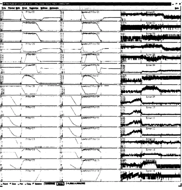
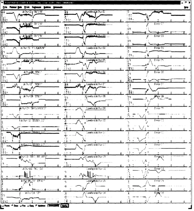
3-4 The waveforms resulting from the initial implementation of DPCS are distorted when the digitizer speed is 10% or more faster than the time required for
calcu-lations. Shot 1040416027 ... 31
3-5 The calculation of the control signals is correct even if some input samples are lost, thanks to the adaptive evaluation of the time stamp of the samples and the use of this information in the PID calculations ... ... . 33
3-6 Plasma control at different cycle rates of the digital control DPCS. The plasma is controlled against vertical instability when DPCS cycle is 100[us (top panel, shot 1050210021) and 200,ts (central panel, shot 1050210022), but disrupts when the cycle is 400us (bottom panel, shot 1050210023) ... ... . 43
5-1 The Graphic User Interface (GUI) ControlMainPanel ... ... . 51
5-2 The GUI Machine with a model of the vacuum vessel, the surrounding structures and the active coils ... . 59
5-3 The GUI DrawFieldPanel. Also shown is the magnetic field on a coarse grid (5 cm step) ... . 61
5-4 The initial equilibrium in the GUI DrawFieldPlasmaPanel ... ... . 63
6-1 Evolution of some physical quantities in the massless simulation ... . 69
6-2 Evolution of some physical quantities in the massive simulation ... . 70
6-3 The initial equilibrium in our simulations ... 71
6-4 The disruption of the plasma toward the upper wall in our simulations ... . 72
6-5 The Simulink block diagram. The power supplies subsytem contains the models of the power supplies. In the simplest case, they are single pole systems, with saturation blocks to limit their output voltages. The blocks implementing the tokamak, the diagnostics and the control system are Matlab sunctions .... . 73
6-6 The subsystem of the power supplies in the Simulink model and a detail of the implementation of the OH1 supply ... 77
7-1 Compression evolution of a perturbed equilibrium for a massless simulation . . . 83
7-2 Compression evolution of a perturbed equilibrium for a massive simulation . . . 84
7-4 Expansion evolution of a perturbed equilibrium for a massive simulation .... . 86
7-5 Asymmetric perturbation, massless simulation ... 87
7-6 Asymmetric perturbation, massive simulation ... 88
7-7 An ideally unstable plasma equilibrium ... ... . 90
7-8 Massive simulation in the case of an ideally unstable plasma ... ... . 91
7-9 Results from the massless simulation of a resistively unstable plasma ... . 93
7-10 Results from the massive simulation of a resistively unstable plasma ... . 94
7-11 Simulation of the plasma discharge for shot 1050804011. The plasma is following the target waveforms of the Plasma Control System (PCS) ... . 97
7-12 Comparison between the real and simulated feedback error signals in the case of shot 1050804011 ... 98
7-13 Comparison between the real and simulated output voltages from the power supplies in the case of shot 1050804011 ... 100
7-14 Comparison between the real and simulated coils currents in the case of shot
1050804011
...
101
7-15 Simulation of the plasma discharge for shot 1050706014. The plasma is following the target waveforms until it disrupts ... 102
Acknowledgements
My years as a student at the MIT Plasma Science and Fusion Center have been exciting. Fusion research is an outstanding example of how interesting physics and challenging
engineer-ing effectively meet. The collaboration with the people who supervised my work, Prof. I.H.
Hutchinson, Dr. S.M. Wolfe and Mr. J.A. Stillerman, has been highly rewarding. Working with them has been always stimulating and a constant opportunity to learn.
The entire staff of people of the Plasma Science and Fusion Center has been equally
sup-portive and important for the successful conclusion of my work.
My brother Luca and my parents Adele and Piero have been, as always, essential to my
accomplishments. My friends Dominic, Thekla, David, Daniel, Sue, Jason, Seton, Luisa, Jenny
and Roberto have made these years human and enriching.
To all of them I extend my grateful acknowledgement.
The present work was sponsored under the contract D.o.E. Coop. Agreement
Part I
DPCS Digital Plasma Control
Chapter 1
Introduction
Alcator C-Mod is a compact tokamak at the MIT Plasma Science and Fusion Center. It is
illustrated in figure 1-1. It comprises a toroidal field magnet (TF in the figure), whose 20 legs
EF1U OH2U
OH1
OH2L
EFIL
Figure 1-1: Illustration of the cross section of Alcator C-Mod
generate toroidal fields up to 8T, 3 central coils, winding around the core of the machine (OH1, OH2U, OH2L) and 10 poloidal field coils (EF1U, EF1L, EF2U, EF2L, EF3U, EF3L, EF4U, EF4L, EFCU, EFCL). It is a feature of the C-Mod coil-set that essentially all the coils are used for both shape and position control, as well as inductive drive. This is in contrast to some designs, such as DIII-D, in which there is a "de-coupled" inductive drive coil that does not affect the shape. Part of the complication of the C-Mod control system in fact derives from this fact, that there is no one-to-one correspondence between parameters to be controlled and single (or small subsets) of coils to use as actuators. The plasma is formed inside the vacuum vessel and a current up to 2MA can be inductively driven by sweeping the currents in the active coils (mainly OH 1 and the OH2 coils). The plasma is ohmically heated and the use of additional radio frequency heating allows the plasma to reach a core temperature of about 5keV. In a magnetic confinement fusion device the exact knowledge of the topology of the magnetic field inside the vessel is essential for studying and controlling the plasma. Detailed information is available from the magnetic sensors. On Alcator C-Mod there are 21 full-flux coils, 6 partial-flux coils, and 118 poloidal pick-up coils. The full-flux coils run toroidally around the machine and measure the magnetic flux coupled with them. Similarly, the partial-flux coils measure the coupled magnetic flux, but they are located nearby ports, so they are not toroidally continuous. Their signals are combined in order to produce the total flux at locations of interest. The poloidal pick-up coils measure the poloidal component of the magnetic field at specific locations around the vacuum vessel. There are four sets of 26 coils, placed at different toroidal locations, plus 14 additional coils. Only one set of poloidal coils is used for plasma control, while the others are for post-processing and equilibrium reconstruction. The other magnetics diagnostics used for control are the plasma rogowski and the toroidal field measurement. Figure 1-2 illustrates the location of the magnetic diagnostics in Alcator C-Mod. The signals from the magnetic diagnostics can be linearly combined in order to obtain the magnetic field at specific locations and information on the shape and position of the plasma. Some of these quantities are chosen as the observables of the system and a number of them are controlled using a feedback loop. Figure 1-3 shows a set of fluxes evaluated at specific locations and used in Alcator C-Mod to calculate the relevant observables. In a standard C-Mod plasma discharge two phases are distinguished, the start-up phase, when the plasma is formed and its current ramped-up, and the flat-top phase, when the
Figure 1-2: Cross section of Alcator C-Mod illustrating the position of the full-flux coils (panel
vu
/top in / out b-ot*sI
~so
Shape Parameters
x
Rg
o (out - in)/IpZC
A'
(top
-
4t)/IP
C-
i"
(t-in
Cl)p
PsX IPSO-RX
i°'
(aOZ
(a(
i
Zi
' ~.(OOZ'
-
/XR
)/Ip
-
'4-
i
)/Ip
0.40 0.!0 0.60 0.70 0.80 0,90 1.00 1.10A possible set of shape parameters
for the plasma
Figure 1-3: The magnetic fluxes at the locations pointed in the figure can be calculated with linear combinations of the responses of the magnetic sensors. These fluxes can then be combined to obtain information on the plasma position and shape. From [1]
plasma current is brought to a stationary value and further experiments are conducted. The
switch time is usually 0.1s. Different observables are used for these two phases. In particular,
in a standard start-up phase of Alcator C-Mod, the only quantities under control are the radial component of the magnetic field at the plasma nominal centroid and the currents in the active coils. After the plasma has been formed, the quantities under control become the plasma radial and vertical position and the inner wall gap scaled by the plasma current (RCUR, ZCUR and CLEARIN respectively), the radial and vertical position of the lower and upper X-points (RXL, ZXL, RXU, ZXU), the plasma density (nl_04), the EF4 current, the plasma current (IP) and the average of the EF2 currents, when the EF4 current (more precisely, the voltage) is used as the corresponding actuator (EF2_BYEF4). While the upper and lower x-point positions are often used as the observables, there are other options, including the strike point locations on the outer and inner divertor plates (STRKPSI and STRKIN) and the distance between primary and secondary separatrices (SSEP).
There is an important distinction between times before and after Os in the first segment of the discharge. Before Os the coil currents are controlled directly, and the only "field" quantity being controlled is BR0, the radial field. No positional or plasma quantities are under control before Os, because there is no plasma then. Shortly after Os, the gains on the ZCUR and RCUR
are turned on, and many of the gains on the poloidal coils currents are reduced or turned off, in
particular those on the OH coils. From Os to 0.1s the feedback on RCUR and ZCUR is used to control the plasma position. The plasma current is normally not controlled by feedback during this time. The observable quantities involving gaps and positions are expressed as products with the plasma current because the products can be simply calculated as linear combinations
of the magnetic signals.
The number of observables that can be ultimately controlled with a feedback loop is related
to the number of actuators which can be independently operated. For the particular case of the shape and position of the plasma, the controllers will be the voltages applied to the poloidal coils or a combination of these voltages. The optimal synthesis of orthogonal controllers for a certain set of observables is a problem which admits purely formal solutions with the tools of control engineering, but an heuristic and physically-conscious approach can be more effective, even if leading to only a non-orthogonal set of controllers [1]. Figure 1-4 shows an example of
combinations of coil currents that can be used to control the vertical and radial position of the plasma.
ZC
R
Two orthogonal controllers for the
vertical and horizontal position
Figure 1-4: An example of two sets of coil currents which form the controllers for the vertical and radial position of the plasma. From [1]
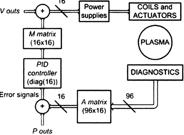
Once the set of observables is defined and the target waveforms for these observables are drawn, the errors between the actual values and the desired values are computed and processed by the control algorithms to activate the corresponding controllers. Alcator C-Mod is currently using a linear control scheme, as shown in figure 1-5. The signals from the diagnostics, that is the magnetic signals, the currents in the coils, the density, the plasma current and other
1
P outs
Figure 1-5: Simplified scheme of the linear control of Alcator C-Mod
V out
relevant parameters, are input to the observer A matrix. The observables are computed as a linear combination of the inputs, then they are subtracted from the target waveforms P outs. Some of the target waveforms must be normalized by the plasma current in order to be consistent with the corresponding observables. The error signals are input to the PID controller. This is currently a set of 16 independent Proportional-Integral-Derivative controllers acting on each wire. The results of the computations are then input to the M matrix, which controls the power supplies of the poloidal field coils, and other relevant actuators, for example the gas valves, which feed-back on the plasma density. The output of the M matrix is corrected by adding the V outs feed-forward waveforms, which provide also the basic control when the loop is open. Detailed description of the plasma control strategies used in Alcator C-Mod have been
previously published [2], [3].
In general, active control is essential for the vertical position of elongated plasmas. In fact, these configurations are obtained with the magnetic field "pushing" or "pulling" on the plasma, the field concavity is directed toward the outboard of the vessel and the zero of the radial field is a position of unstable equilibrium. Even a simple physical picture proves this assertion: if the plasma centroid is slightly moved from the zero of the radial field, the plasma will experience a force in the same direction of the displacement, instead of a restoring force. However, if the plasma is close enough to the wall, the passive currents induced in the metal structures will slow the instability down to their resistive decay time: this regime is called resistively unstable and provides a margin for active control, which would otherwise be impossible in the regime of ideal instability, where the vertical run is damped only by the natural inertia of the plasma, with typical times of < 100ps. In the case of a resistively unstable plasma, this time becomes a few ms. The fast poloidal coils EFC are used in Alcator C-Mod to compensate the vertical instability of the plasma: they are connected in anti-series and are fed by a chopper power supply. The small signal bandwidth of the supply is 1500Hz, but falls to about 300Hz at full
power.
The control scheme of Alcator C-Mod was originally implemented using a hybrid digital-analog system Hybrid [3]. During the 2003-2004 campaign and in the summer 2004 the new Digital Plasma Control System (DPCS) was implemented and successfully tested off-line. Dig-ital control systems have been implemented on many tokamak machines, for example DIII-D,
JET, JT-60U, ASDEX-U, TCV, because of their flexibility and reliability. Part of the interest in digital control comes from the development of the next generation tokamaks, among which the International Thermonuclear Experimental Reactor (ITER), whose size and power handling will require considerable safety measures and optimization procedures [4], [5]. Digital systems also allow to run advanced control strategies to stabilize high performance plasmas [6], [7], [8],
[9].
The initial goals of DPCS were the consistency with the control signals produced by Hybrid, the compatibility with the MDSplus data structures created for previous shots, so that these shots could be reloaded and run with the new system, and the compatibility with the general control software PCS (Plasma Control System) and its graphical user interfaces. MDSplus is the database structure standard for fusion experiments [10].
At the start of the 2005 campaign DPCS was used to control the real machine and has been in operation since then. In fact, some advanced features have already been implemented or tested, such as the allowance for the loss of input samples, the real-time compensation of the input offsets and the reduction of the cycle rate for extra headroom for computation. The following chapters describe the architecture of the previous control system Hybrid and the digital control system DPCS. The off-line debugging of DPCS and the first operation of DPCS
Chapter 2
Implementation of Hybrid
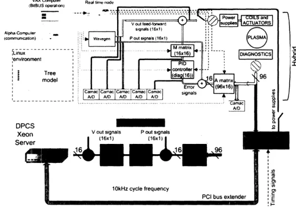
Figure 2-1 illustrates both Hybrid and DPCS. Hybrid hardware is mainly composed of arrays of
VAX Cputer Real time node
1RitRt Iq nrat-i Alpha Co (communi rLinu :envii I ;I I I- i_ DF X4 Se I'M. ..Q '-r
J
U P 10kHz cycle frequency CI bus extenderFigure2-1: Complete schematic of Hybrid and the current implementation of DPCS -I I 0 , co
,
Cn or , O El
the reference pin and the output is the input multiplied by the digital word stored in the DAC. Some drawbacks exist with this implementation, for example the leakage between input and output at zero gain, or the presence of a finite output for zero input. The overall system has performed satisfactorily for its 14 years of operation. Among the advantages are a large analog bandwidth (about 20kHz) and a low noise background. The bandwidth is largely exceeding the speed of the power supplies (always below kHz, except for the fast EFC coils) and the time constant of the coils, with their large inductances and small resistances.
Hybrid is real-time, meaning that matrices and references are switched during the plasma discharge, but it is not adaptive, which means that the order of the matrices and references are decided and set before the shot, according to the particular plasma configuration under investigation. In theory, Hybrid could operate adaptively, but this feature has never been implemented.
The structure which contains the information to run a shot and stores the data from the shot is the MDSplus tree. MDSplus trees are used for control, data acquisition and analysis of essentially all aspects of the C-Mod experiment [10]. The matrices and the parameters to generate the P outs and V outs are pre-loaded into the multipliers and the wave-function generator through a BitBUS fieldbus. The fieldbus is managed by a VAX computer and the communication between the Linux environment and the VAX is operated by an Alpha computer. When a shot is run, a trigger signal is sent to the timing node, which takes care of sequencing the various phases of a plasma discharge by issuing the switching of the references and the matrices. The different instances of A, M and PID matrices are thus applied at different times during a plasma discharge. The system was originally developed by the TCV group as a clone of the hybrid control operating on TCV [11]. The data from a discharge are digitized with a sampling rate of 500Hz and stored into the corresponding tree.
Chapter 3
Implementation of DPCS
The decision to implement a new digital control system is consistent with the work done on big devices, such as JET, JT-60U, DIII-D, but also on smaller machines: a significant example is the TCV in Lausanne [12], whose earlier hybrid control system was a twin of C-Mod Hybrid.
The essential hardware of DPCS is extremely compact. It comprises two CPCI cards, a CPCI to PCI bus extender and a XEON Server. Each I/O card has 64 16-bit inputs and 16 analog outputs, totalling 128 inputs and 32 outputs. Cards with more channels or additional cards can be added should the need arise. The original hybrid control computer had a total of 96 inputs and 16 outputs. The server is a standard Intel® XeonTM 3.20GHz with 2 Gigabytes of memory. t can easily be replaced or upgraded since it is completely standard. The computer is running the RedHat Linux distribution, booted diskless over NFS. The system boots using dhcp and PXE.. A local disk is present for paging and swapping when not in real-time mode. The PCI/CFPCI extender card transparently makes the CPCI cards appear as PCI peripherals
on the host computer. The one in use is a 32 bit 33 MHz card from SBS Technologies, 64 bit 66 MHz cards are available should this prove to be a bottleneck in the future.
The DPCS software consists of many IDL routines grouped in the file DPCS startup.pro [13]. The communication of DPCS with the main system supervising plasma discharges is
illustrated in figure 3-1.
The software operation is summarized in the following:
4
4
INIT CHECK PULSE RECOOL ... INIT CHECK PULSE RECOOL. DPCS M server Hybrid dpcs init dpcs_realtime dpcsstore ,... dpcsinit dpcsrealtime dpcsstoreFigure 3-1: Schematic of the communication between the real time control routines of DPCS and the main system which supervises the plasma discharges
PLC State Machine STATE Computer DISPATCHER . .
computer is restarted). This script initializes the digitizers, starts up an MDSplus server process, and starts an IDL process running dpcs.pro.
2. dpcs.pro compiles dpcs_startup.pro, the file that contains the main IDL routines. It then invokes the dpcs_ startup procedure, which locks down memory, initializes the low-latency interface to the hardware, and exercises the interrupt disabling. On return from dpcs_ startup the dpcs routine sets up the fifo buffer through which communication be-tween the server and the IDL process is carried out.
Steps (1) and (2) are normally done once a day. The remaining steps happen every shot.
3. During INIT (actually during the transition from RECOOL to INIT), the dispatcher sends the ACTION \HYBRID::TOP.HARDWARE.DPCS:DPCS:INIT_ACTION to the MdsPlus server running on pcdaqdpcsl. The server carries out the DPCS__INIT method which instructs the IDL process to execute the routine dpcs_ init. This routine sets up the parameters used by the dpcs_ real_time and dpcs_ store routines, based on information read from the MdsPlus tree. The parameters for the real-time calculations, including matrices, target waveforms, etc., are all passed using IDL pointers to heap variables. The
logical steps done in dpcs_ init include:
a Read from the tree the names of software packages to be run. This includes all calcu-lations to be done other than the main routine which emulates the hybrid.
b Clean up after previous cycles which may not have terminated correctly. This avoids potential memory leaks and dangling heap variables.
c Read from the tree the parameters of the main calculation, i.e. the cycle time, the shape of the matrices that emulate the hybrid, and then the matrices and target
waveforms themselves.
d Call the initialization methods for the auxiliary routines, which set up all the para-meters for those calculations. Also, compile all the real-time executables for those calculations.
f Initialize array variables to hold the results of the real-time calculations at each time-step; these are eventually stored in the tree by the dpcs_store routine.
4. During CHECK (actually during the INIT to CHECK transition) the dispatcher tells the MDSplus server on pcdaqdpcsl to execute the DPCS RTACTION method. This method causes the server to invoke the dpcs_ real_ time procedure in the IDL process. This procedure executes a dummy pass through the real-time calculation, which causes all the necessary instructions and variables to be faulted into memory. It then disables the interrupts and waits for a trigger before transferring data from the digitizers. The trigger and clock are fired in the PULSE state using CAMAC modules. The real-time loop is synchronized to the digitizer clock. If no trigger is received after a pre-set number of polling cycles the real-time code exits with a timeout error and re-enables the interrupts. Otherwise, the code executes the loop (write the output from a previous iteration, read the new input and perform the computation) until the termination condition is reached, at which the interrupts are turned back on and the real time routine is exited. For the detailed comment of the real time routine see also section 3.2.
5. During RECOOL (actually during the PULSE to RECOOL transition) the dispatcher tells the MDSplus server to execute the DPCS_STORE action and the IDL process runs the dpcs_store routine. This routine stores the digitized input data and the results of the real-time calculation to the MDSPlus tree. The routine also calls individual STORE routines (methods) associated with any auxiliary calculations carried out. Finally, the heap memory associated with the calculation parameters is freed.
6. Also during RECOOL the dispatcher tells the server to execute the RT_CHECK action which examines the results stored by the store action for discrepancies and optionally
broadcasts a message if any are found.
3.1 Benchmarking and debugging DPCS
The initial requirements on DPCS were that it perfectly emulate Hybrid and reproduce the Hybrid signals during a plasma discharge. During the 2003-2004 campaign the signals
digi-tized from Hybrid were compared with the corresponding signals from DPCS, in the case of successful plasma shots, power supply test shots and fizzle shots. Many simulators have been implemented i IDL to investigate particular aspects and separate the various contributions of the discrepancies between Hybrid and DPCS. At the same time, many MDSplus dwscopes have been designed to allow rapid estimation of those discrepancies. In our analysis a time-varying discrepancy of a few percent of the time-varying component of the corresponding Hybrid (or DPCS) signal was considered acceptable. Also, the analog offsets of Hybrid were subtracted from the Hybrid signals before comparing them with the results of DPCS1. The main results
are summarized in the following and refer to an early implementation of the DPCS hardware comprising three 32 channel input digitizers and a Pentium 4 PC running the IDL code. No output cards were present and the output routine was not implemented. Despite the different configuration and performance of the hardware, this system was perfectly adequate to test the
main features of the DPCS software2.
* A systematic time delay of 1ms was found between the Hybrid and DPCS A_in, that is the digitized versions of the input signals. This time delay is exactly half of the period of the CAMAC digitizers of Hybrid and is due to the fact that Hybrid was sampling on the falling edge of its clock, while the time stamp was taken on the rising edge. This detail is in itself insignificant, but must be compensated when the signals from Hybrid and DPCS are subtracted to evaluate their discrepancies.
* The Pouts of DPCS and Hybrid matched very well, as shown in figure 3-2. An impor-tant error was found in the algorithm which interpolated the DPCS references from the minimal data stored in the tree. The references are programmed in the PCS graphical user interfaces by adding points on x-y displays. These points are then interpolated in the init phase, before the discharge begins, to produce the continuous waveforms which
l In the present chapter we use the convention of calling the outputs of the A matrix A_outs, the reference
signals P_outs, the sum of A_outs and P_outs error signals (or, simply, errors), the outputs of the PID matrix
PIDouts, the outputs of the M matrix M_outs and the feed-forward signals V outs. The inputs of the A
matrix are called A_ins. The differences between PCS and DPCS signals are referred to as discrepancies and
they usually have an offset and a time-varying component. Our conventions must not; create confusion with the
experimental data: in the tree A_out is used to indicate the error signals (A_outs + Pouts) and M_out is
used to indicate (M_ outs + V_outs).
2
control the machine. However, during a plasma discharge, the observables are switched according to the particular phase, for example current rise or flat-top, and the target waveforms are accordingly changed. The event is called segment switch. Because some of the wires refer to completely unrelated quantities, there may be abrupt changes in the references. If these changes are interpolated across a segment switch, they will give rise to glitches. In order to fix the problem, an additional point is added one tick before each segment switch, before the linear interpolation is done.
* The A matrices were compared with the help of a simulator which applies the inputs of Hybrid to DPCS, performs the computation (A matrix + Pouts) and evaluates the discrepancies between the real Hybrid error signals and these simulated error signals. The simulator points out the differences between the matrices, given the good matching of DPCS and Hybrid P_outs. The simulator demonstrated that a little change in the gains, as small as a few percent, may sum up in a big discrepancy between DPCS and
Hybrid error signals, as high as 30%. However, the differences in the gains were of no concern because DPCS was going to replace Hybrid in the feedback loop. A leakage was also discovered in some outputs of the A matrix of Hybrid, where the gain is set to zero
but the output has a small signal. These small signals, as well as the offsets of Hybrid, are eventually integrated over time in the PID controller and cause big errors at the output of the PID of Hybrid. Of course DPCS doesn't have this kind of flaw. Figure 3-3 illustrates this issue.
* The PID matrices worked very similarly, in spite of the simple discrete implementation of the derivatives and integrals in DPCS. A second simulator was implemented to test the PID matrices, which works in a way very similar to the A simulator, except for the fact that the Hybrid A_outs must be expanded on the DPCS time base, before applying them to the DPCS PID. This is necessary, because the DPCS PID calculates derivatives and integrals on the DPCS time base. The simulator allows the user to tune the time constant of the integrator Tint and the best matching between Hybrid and DPCS was obtained with
Tint = 0.095. The current value of Tint in DPCS is 0.08. A major advantage of DPCS
integrate offsets, because DPCS does not have the problem of analog offsets.
* The feed-forward signals V_outs of Hybrid and DPCS matched very well and the inter-polation problem at segments switching was fixed for V_outs too.
* The M1 matrices were compared using the M simulator, which is similar to the A and PID simulators described above. The signals (M_outs + V_outs) agree very well, but DPCS doesn't show the saturation problem of Hybrid.
All the simulators mentioned above use the IDL code of DPCS with the necessary modifi-cations. The A and M simulators have also been implemented with a different and easier IDL code. The results from the different implementations agree perfectly and this proved to be a
good test of the IDL code.
In conclusion, we found that DPCS was following Hybrid and was producing signals with the same shape, within a few percent, except for offsets, saturation and other Hybrid non-idealities.
3.2 DPCS real time code and time performance
The initial implementation of the IDL procedure dpcs_ real_ time used two nested for loops to read the samples and perform the corresponding calculations during the shot, with the appropriate time evolution of matrices, waveforms, and integrators and derivatives parameters. The period of each sample was fixed to 100ps (10kHz sampling rate). This version of the code was tested fr over three months without revealing any significant bug. In order to test its time performance, a number of performance parameters were added in the tree. The most important
are:
* NTIMES is the number of input samples which have been read and processed by the IDL real time routine. NTIMES is the dimension of the vector tlatch, which contains the latch times of the input samples.
* TLMAX is the max value of the vector tlatch (the time of the last sample). * TLMIN is the min value of the vector tlatch (the time of the first sample).
W V 115,
fow~
fr*',"~-;j-
~
"~'~,
I
:: 0>~~~~~~~~~~~~~~~~~~~~~~~~~~~~~~~~~~~~~~~~~~11 19 1' U!e...
,, S----.-,,,,_ ,, ,, ..., ,·.. ...
_.
,,_h~
,
- 4 ; ',, ,- ,I llrrill~l wilt ,ILl
1 0
1 ...
'
g h
@E
_
_
i ', t' i " -Or] ---- ---- !N I ' ' ",,I no_A.
U
IIIliiE
f i__ ___g t w U - 2, ;4 ' " ...4: '--, ~~ '". 4 ;.; / -- ---X
,- -
- - . - \ - -- - r --- --- _- ' ft rr~ :O i - .. f ...,1s~~~~~~~
gg4
-..4.
..,
-m~w - -F-- sa >tS - en B'T-f
I
.e ~ ~~~~~~~ '.!.
4 ,.1 -, ' -- * _- x,!F ! E > > -'e / ____ __ __ _ t____--__ ____ _____ ___ -_ -i_ _;.____ luI P
Figure 3-2: Hybrid and DPCS Pouts (reference signals) and the error between them for shot
1040325005
I I I III III I I I
Figure 3-3: Note the leakage of Hybrid hardware during the second segment of the discharge, that is after 0.1s, in signals 11 and 12. The leakage causes the error signals to be non-zero even when the gain is set to zero (i.e. all the coefficients of the A matrix should be identically zero). DPCS is a digital system and does not have this kind of problem. Shot 1040325005
*
TINT_ MEAN is the average value of the time intervals between consequent input sam-ples. In the case that no samples are lost, TINT_MEAN is exactly the clock period.*
TINT_ MAX is the max value of the time intervals described in TINTMEAN.*
TINT_ MIN is the min value of the time intervals described in TINTMEAN.*
TINT_ STDEV is the standard deviation of the time intervals described in TINTMEAN.*
STATUS is a variable used to check the loss of input samples, which occurs when the computations in the loop are too slow with respect to the rate of the digitizers. The variable STATUS is indeed the combination of three tests, namely NTIMES > 0 (i.e. at least some samples have been processed by DPCS), TLMAX > TLMIN (i.e. no colossal errors in the time base and TLMAX TLMIN) and TINT_MAX < 2 *ACTDELTAT.
This last condition checks that no samples were lost. In fact, the sampling period of the digitizers is specified by the entry DELTA_ T in the tree. Because the period can only be a mul-tiple of the 1ps digitizers clock, a new variable ACT_ DELTA_ T is evaluated from DELTA_T and stored in the corresponding node in the tree. STATUS checks the loss of samples because this event happens only if there is at least one couple of processed samples whose time inter-val is larger than twice the digitizers period. The initial speed tests were done by changing DELTAT in the tree. The system could get every sample and process it correctly up to a limit sampling period of 45ps. With 40s about 10% of the samples were lost and the output
waveforms were seriously distorted (figure 3-4).
This happened because the calculations assumed the theoretical ACT_DELTA_T stored in the tree, while the actual time delay between the input samples was not constant.
Since the first implementation, the DPCS code and dpcs_ real_ time have undergone many upgrades in order to improve the robustness, efficiency, flexibility and readability. In particular:
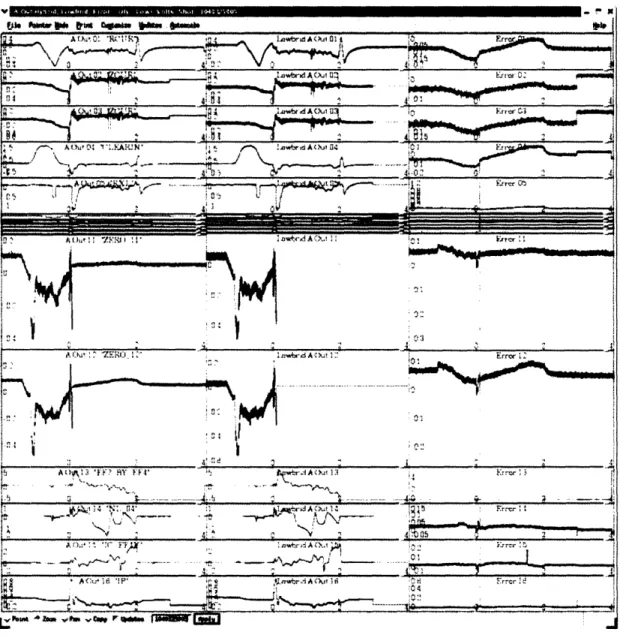
* in order to make the system more robust with respect to the loss of input samples, dpcs_ real_ time takes into account their actual time stamp. Figure 3-5 shows an ex-ample of the A_outs waveforms calculated with the adaptive version of the code, when
[v MMM p 4 4
47~~~~~~~~~~~~~~~~~~~~
U 4~
~
~
~
, .. *... .. !,I CI 4! IAV 4 4 ! ' . 4 A ,, 4 4s -
-~~~~113-,- 4~~T1
~ ~
177 FTV.4-,jA 4Y fk'.,..;.__,.__, ..
...
i~ :~Ak;
.
4~1. , -:,rr-.'- 4:' /~~~~~~~~~/ 't' "-- ----
--
'~ . . . .'~ '.____
,I . , - .4 - -. .- 4 -+xI~~~~~~: . A . . . .- ,0e = ...;~
--
4,-,---.-'~...'"--
,...
...-
"
"....
Figure 3-4: The waveforms resulting from the initial implementation of DPCS are distorted when the digitizer speed is 10% or more faster than the time required for calculations. The error signals in the third column show that the outputs of DPCS/Lowbrid (second column) are
significantly different from the correct control signals (first column). Shot 1040416027
lot I DW ft- 16 triffit 010- 9"M -t*
i
L ft"
. am . Fe* . a" PI 100" I = amabout 10% of the input samples is lost. The waveforms are correct and do not show the
distortions in figure 3-4.
* Custom procedures can be called within the loop to perform additional computations at any stage, for input conditioning, observers estimation, PIDs correction or controllers syn-thesis. All these operations are implemented within a unified syntax, the call_procedure instruction, whose parameters are appropriately designated.
;~ -~-'--
...
...
Il II II~
IIII
IIII
Jill
II"~'x
r~~~ . ... ._
~~
4 4~~~~~T;q... ... '" tl~~~~~~~* 640N %" t*M4 gOP, S 4,' ,' . A CXL~ '~~~~~~~~~~~~~~AI~ ~ ~ ~ ~ ~ ~~~'
~
~ ~'~
' ' *r4 A)~ J5 ' ""____.________A00' 11 I11 N', -AL f, iA .I
,C ,O
~ ~~~~~~~?
.. . .A')u r 'Tr. ''' i; 2 2 K -42 + C S I ^ n ^; O i _ - ., [A :.'4,, 4 I _ ,, . A~~~~~~~~~~~~l~J. toIr 'z. " A~ us lwj l. la'~m ~ M N4.; * 4 * .a ---- - , . 4 k, j._ -Y- ---m. . .Fr .. r.. a -4 -s->X -~s--- --- A I# 6 Ls~
4 h P, t. t ,~ wT , ;? IK',_,~~~~~~~~
. % r. v*,. ~,! 4, ~'I,~ ,' ...Figure 3-5: The calculation of the control signals is correct even if some input samples are lost, thanks to the adaptive evaluation of the time stamp of the samples and the use of this information in the PID calculations. In the case illustrated above 10% of the input samples was lost because of the delay in the loop calculations, but the DPCS/Lowbrid signals (second column) are still consistent with the correct control signals (first column), as the error signals (third column) show
The dpcs_realtime
code, as in use in June 2005, is included and commented
below.
pro dpcsreal_time,maxloops
common hybridparams,MAXSTEPS,dtl, dt2,NW,NX,NM,NSEG,SEGNM
common DPCSparams,Nbuf,Ndacs,Ncards,ecm common hybrid_wavegen,pP,pV
common hybridoutputinfo,XOUT,YOUT,UZOUT,U_ ,P-OPOUT,VOUT,LAST_STEP, $
tlatch,tinst,tprocess,hbpoll
common hybridinitc,pswcommon,swunion,interrupts
common hybrid_daq_data,buf,dacs common DPCS_software, llImage
common dpcsfunctions,inputfuncs,observerfuncs,controller_funcs
common dpcsprocedures, inputpros,observerpros,pidpros, controllerpros, $
testpros,Allpros
common dpcsprocedureparams,inputparams,observerparams,pid_params, $
controllerparams,testparams
The initial part is used for declaring common variables. These are organized
according to their specific functions: hybrid_params
contains the definitions of
the parameters of the Hybrid-like control, that is the maximum number of time
steps during a discharge MAXSTEPS (this is evaluated on the basis of the trigger
time, the stop time and the DPCS sampling period), the derivative and integral
time scalings dtl and dt2, the number of wires (observables) NW, the number
of inputs of the A matrix NX, the total number of inputs Nbuf (NX and Nbuf
used to agree on Hybrid, but this is not necessarily the case with DPCS), the
number of controllers NM, the number of segments active in a plasma discharge
NSEG and their numeric identifiers SEG_NM. DPCS_params contains
parame-ters specific of the hardware of DPCS, the total number of inputs Nbuf, the total
number of outputs Ndacs, the number of I/O cards Ncards and the number of
ticks of the clock of the digitizers corresponding to a DPCS cycle ecm. pP and pV
are the pointers to the target and feed-forward waveforms (P outs and V outs).
XOUT, YOUT, ZOUT, U_OUT, POUT, V_OUT, LASTSTEP, tlatch,
tinst, tprocess, hb_poll are used to store momentarily the signals that will be
written in the tree by another routine, dpcs_output: XOUT, YOUT, ZOUT,
UOUT, P_OUT and VOUT store the inputs, error signals, PID outputs,
con-troller outputs and target and feed-forward waveforms for each time step. The
time step itself is in tlatch. The other three time parameters, tinst, tprocess,
hb poll, are used for debugging. hybridinit
c contains the definition of the
switching times of the matrices and waveforms during a discharge. interrupts is
used for disabling the interrupts in the real time loop. hybriddaq_data
contains
variables used to pass inputs and outputs to and from dpcsinput.
11Image
is the
low-latency routine used to operate the input cards in fast data acquisition mode.
Finally, dpcsfunctions and dpcsprocedures contain the definitions of the
pro-cedures and functions that can be called to perform custom computation at each
stage of the control loop.
; first time though fault in all of the code message, /reseterror_state
sw = sw_union
psw = psw_common nj =nelements(sw)-1
; Initialize internal variables for more efficient assignments in loop y=fltarr(NW)
yl=y
yldum=y \qquad \qquad \qquad ;NEED THIS FOR REAL TIME STEP
ylast=y
y2=y y2_last=y
real_step=1. \qquad \qquad ;NEED THIS FOR REAL TIME STEP z=y
x=fltarr(Nbuf)
NXml = NX-1 ; Note x is now dimensioned to conform to the shape of buf, not A
p = fltarr(NW)
q = p \qquad ; Make a dummy var for just the observer, same size as P v = fltarr(Ndacs) ; Could take U and V to be fltarr(Ndacs). It is not NW
u = v \qquad U and V must have same dimension, (or n_U>n_V) to avoid out-of-range w = v ; Make a dummy of the same length
sp = size(*pP) ; *pP and *pV are dimensioned in dpcsinit and may have different lead sv = size(*pV) ; dim than local 1-dim variables P and V
Np = sp[l] & Npml=(Np<nelements(p))-lL
; Used for subscripting. Upper bounds must avoid out-of-range Nv = sv[1] & Nvml=(Nv<nelements(v))-lL
tl = lonarr(Ncards) ;tl and ti are now local variables passed to dpcsinput
ti = lonarr(Ncards)
tp = lonarr(Ncards)
hbpoll = lonarr(Ncards)\qquad
; Implement a synchronous loop over switch times ; Initialize counters and flags:
step=Ol
first = \qquad ; Set flag indicating first pass through RT loop
iO = sw[O] ; This is probably always zero? i = sw[O]
j =0
exited_early = 0 EXIT_I = sw[nj]-1 EXITS = MAX_STEPS-1 max_loops = long(maxloops); Get info on external real_time procedures
Ninp = nelements(inputpros) & Ninpml = Ninp-1 & $
callinputs = (Ninp gt OL)
Nobsp = n_elements(observerpros) & Nobspml= Nobsp-1 & $
call_observers = (Nobsp gt OL)
Npidp = nelements(pidpros) & Npidpml= Npidp-1 & $
call_pids = (Npidp gt OL)
Ncontp = nelements(controllerpros) & Ncontpml=Ncontp-1 & $
call_controllers = (Ncontp gt OL)
Ntestp = n_elements(testpros) & Ntest_pml=Ntest_p-1 & $
call_tests = (Ntestp gt OL)
After the initial definition of the common variables, some of them are initialized
and the external ones are copied into local variables to make the code faster.
The counters and flags for the loop are initialized and the information on custom
procedures is retrieved.
REPEAT BEGIN
x[O] = dpcsinput(first, maxloops, timeout, tl, ti, tp, hbpoll) ; Need to avoid out-of-range for NX<Nbuf below,
; in which case, not subscripting the LHS is more efficient IF (not timeout) THEN BEGIN
inc = tl[O]/ecm i = inc+iO
The real time loop is contained in the REPEAT-UNTIL instruction. dpcs_input
reads the array of 128 input samples (in the current implementation of DPCS
there are 128 input channels, each digitizing at 16 bit resolution). This instruction
calls a custom C routine, llAcquire, which waits for the inputs and performs a
time-out check by polling for the trigger for a maximum number of iterations
max-loops. The inputs are passed through the common variable buf. If the trigger
doesn't show, the variable timeout is set to 1 and the loop is exited. The time-out
check cannot be based on the internal clock of the DPCS computer, because the
interrupts are disabled during real-time operation. The reason for doing this will
be explained later in the comment of the code. The input instruction also returns
the time stamp of the samples, tl, and other timing parameters ti, tp, hbpoll. ti
is tl plus the transfer time from the input cards to the computer. In the case
dpcs_input doesn't time-out, an incremental index is calculated on the basis of
the time stamp tl (inc = tl[O]/ecm). dpcsinput also sets the analog output values
in the call to llAcquire. The common variable dacs is used to pass the outputs to
llAcquire.
IF (i gt EXITI) THEN begin
exited_early = 1
goto, EXITEARLY ENDIF
The target waveforms, feed-forward waveforms and matrices will be accessed
using the real time indices inc and i, instead of a simple incremental pointer.
The adaptiveness with regard to the real timing of the inputs is one of the most
interesting features of the code and has many advantages: for example, a number
as large as 10% of the total input samples can be lost and the control signals are
still correct. It required careful implementation though, for example the branch
instruction EXIT EARLY had to be introduced to account for the case when some
samples are lost and the maximum number of iterations EXITS is not completed
in the time of a discharge. The exit early condition is based on the real time pointer
i.WHILE (i ge sw[j+1]) DO j++
The processing of input samples according to their real time stamp brings
an-other issue, when the real time index i is pointing to a time past a reference or
matrix switch, but the matrices and waveforms haven't been updated yet. The
solution to this problem employs a WHILE cycle. The real time index i is
com-pared with the set of indices which mark the times at which the matrices and the
waveforms have to switch. The pointer to the matrices and waveforms j is updated
until i becomes smaller than the next switching index.
; Index into P and V arrays, based on real timestamp and lead dim of array sNp = inc*Np
sNpl = sNp+Npml sNv = inc*Nv sNvl = sNv+Nvml
The
target
waveforms
and
feed-forward waveforms are read using the real time
indices sNp - sNpl and sNv - sNvl.
; Optional input conditioning step IF (callinputs) THEN $
FOR k=OL,Nin_pml DO callprocedure,inputpros[k],*inputparams[k,j], x ; Update the target vector from the P waveform
; The reference could be generalized
p[O] = (*pP)[sNp sNpl] * ([10.,x[55]])[*psw[6,j]] ; Observer Step
q[O] = *psw[O,j] # x[O:Nxml] ; Multiply the inputs by the A-matrix IF (callobservers) THEN $
FOR k=OL,Nobspml DO $
callprocedure,observerpros[k], *observerparams[k,j] ,x,q
y[O] = q + p ; form the error signal realstep = (tl[O]-t_last)/ecm
yl[O] = (realstep ne OL) ? (y - ylast)/dtl/realstep : yldum ; Derivative value y2[0] = (y2_last +realstep*dt2*y * *psw[3,j]) * *psw[5,j] ; Integral value
t_last = tl[O] ;NEED THIS FOR REAL TIME STEP
Z[O] = *psw[2,j] * y + *psw[4,j] * yl + y2 ; PID step (default linear gains) IF (callpids) THEN $
FOR k=OL,Npidpml DO callprocedure,pidpros[k],*pidparams[k,j],y,yl,y2,Z
v[O] = (*pV)[sNv sNvl]\qquad \qquad \qquad ; This step's V (of whatever length) w[O] = *psw[l,j] # Z ; Product of M#pidout, perhaps with trailing zeros
IF (callcontrollers) THEN $ FOR k=OL,Ncontpml DO $
callprocedure,controllerpros[k],*controllerparams[k,j],Z,w
U[O] = v + w ; The sum is of the right length (nu=nv=nw=Ndacs) IF (calltests) THEN $
FOR k=OL,Ntestpml DO $
call_procedure,testpros[k],*testparams[k,j],x,p,q,y,yl,y2,Z,v,w,U The computations of the PID are reported above. Note how the time step of
integrals and derivatives is including the information on the real time step. Another
important feature of DPCS is the ability to accommodate custom computations at
various stages, for input conditioning, observers estimation, PIDs correction or
controllers synthesis. All these features are implemented within a unified syntax,
the call_procedure instruction, whose parameters are appropriately designated. In
particular, the input conditioning routine is used to compensate the input offsets.
dacs[O] = 10.< U >(-10.) ; use [0] subscripting for dacs vector allocated in dpcsinit dpcsoutput, step,tl,ti,x,y,Z,U,p,v, tp, hbpoll
; Could try doing these directly, using pointers? step++
The final output is constrained within the power rails of the output cards. The
content of dacs will be output at the next call of dpcs_input. The output
rou-tine dpcs_output saves the current results in the common variables LAST_STEP,
tlatch, tinst, X_OUT, Y_OUT, Z_OUT, U_OUT, P_OUT, V_OUT, tprocess
; after the first time through the loop disable the interrupts
IF (first) THEN BEGIN
IF interrupts THEN josh = callexternal(llImage, 'llDisableInts')
first = 0
; step-- ; step back to zero, so dpcsoutput overwrites dummy values ENDIF
ENDIF ELSE GOTO, timeout
Deterministic time performance is obtained on a PC running a standard Linux
operating system by disabling the interrupts: no instruction in the control loop
will be interrupted and it will take a deterministic time to complete. In order to
avoid problems of page faults, a first cycle through the loop must be completed
and the relevant instructions and variables loaded in the internal memory of the
processor, before the interrupts are disabled.
ENDREP UNTIL (step gt EXITS) ; Normal Exit when last step ; all done so enable the interrupts
; and leave low latency mode
EXIT_EARLY: ; Exit when get to last timeslice earlier than num steps timeout: ; Timed out waiting for trigger
IF (not first) THEN begin IF interrupts THEN begin
dummy = callexternal(llImage, 'llEnableInts')
spawn, /etc/rc.d/init.d/ntpd restart > /dev/null' ; reset the date ENDIF
IF (timeout) THEN print,'Timed out'
IF (exitedearly) THEN print,'Exited Early' ENDIF
The interrupts must be re-enabled only in the case that two or more cycles of
the real time loop were completed.
dummy = call_external(llImage, 'liDone') ; Clean up Heap Variables
ptrfree,pP,pV,psw
LASTSTEP = STEP-1 ; Needed so that Store knows how many to store
print,'LASTSTEP=',LASTSTEP, 'EXITI=' ,EXITI, 'EXIT_S=' ,EXIT_S
print, 'i-' ,i, 'step=' ,step
help, /structure, !errorstate end
The final cleaning and log operations after the control loop.
In spite of the large number of input and output channels, the basic PID controller cycle uses only 48/us, which correspond to an headroom of about 5 0/1s for extra computation at the nominal rate of 10kHz. This controller was used in the power supplies test day (run 1050204) and in the early conditioning of the machine. With various upgrades, DPCS has been on-line since the start of the 2005 experimental campaign. An initial tweak-up of the programming of
previously run discharges was necessary but the new config files are likely to work on DPCS
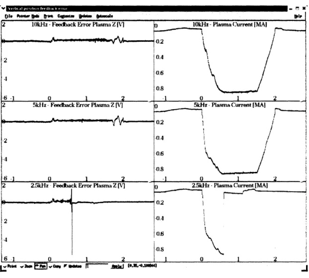
consistently in time, as the implementation of DPCS is inherently free from drifts and other problems of analog circuitry. The run 1050210 was in part dedicated to test one of the new features of DPCS, namely the possibility of changing the cycle time to verify the limit speed at which the plasma can be controlled against vertical instability. At the nominal speed of 10kHz, DPCS has an equivalent bandwidth below 5kHz, while the EFC coils, which compensate for the vertical instability of our plasmas, have an analog bandwidth of about 3kHz. We tried to reduce the DPCS cycle time for a rather unstable plasma. The ratio of the decay index and the single mode critical index for this plasma was nxxc = 1.15 and the elongation was k = 1.68: these values are close to the limit of controllable plasmas in Alcator C-Mod. The peak current was 0.8MA. The plasma was successfully controlled at 10 and 5kHz (discharges 1050210021
Notably, the plasma could almost be controlled at 2.5kHz, thus we expect the minimum cycle
., (kHz -Feeidmb ck FError Plasma Z [VI 02 5k1Hz -Plasma Current [IMA
-046
... n-0~ .... ,A/_\ 02
1
~~-2 ~~~~~-1.o4
i~~~~~~~~~~~~~~~~/
-0.8 ....
,-6 -1 1 _,
2. 5j-k~z - Feedback Error Plasma Z I 2.5liz Pasma (urren [MAI , -o] 1~~~~~~~~~~~~.
1
~~ ~ ~ ~~~~~~~~~-a.
i
1~~~~~~~~~~~~~~~0.6
I6'<
)
_,____________________ _o 1 ? I i,6 .;i . 0 ....1 ? 0 , 1 ?L:%m 'W am
EtI
-wat or - - Aal (oe.4."sOhJ
Figure 3-6: Plasma control at different cycle rates of the digital control DPCS. The plasma is controlled against vertical instability when DPCS cycle is 100,us (top panel, shot 1050210021) and 200,us (central panel, shot 1050210022), but disrupts when the cycle is 400,ps (bottom panel, shot 1050210023)
rate for this type of plasma to be slightly above 2.5kHz. At 5kHz the headroom for extra computation is considerable, about 150/As.
I I i i i I r ---11 . - -- r- - : ;. I
Part II
Alcasim simulation
code for
Alcator
Chapter 4
Introduction
Alcasim is a code developed in Matlab-Simulink with the intention of providing a flexible tool for the analysis of control strategies for a tokamak. The application of the powerful duo Matlab-Simulink for modeling a plasma discharge in a tokamak and studying the associated control
issues is not new, for example [15] and [16], where the DINA simulation code is integrated for
modeling the tokamak and the plasma. In particular, the suite of tools developed by people at DIII-D provides a powerful environment for design, simulation and study of tokamak control, both for devices that already exist, like DIII-D, NSTX, and MAST and for those which are in the design/construction phase, as demonstrated in the case of KSTAR, EAST and ITER [17]. Nevertheless, in the cases mentioned above, the code is intended to simulate the control of a plasma in equilibrium, while incorporating a detailed description of the physics of the plasma and the various components of the machine. Alcasim uses a discretized electromagnetic model of Alcator C-Mod and a single or multi-filament plasma, as discussed in [18] and [19], and can simulate full discharges, comprising the current ramp-up and current ramp-down. The results are consistent with the experiments of C-Mod, when the same setup and control parameters are used. With Alcasim we tried to meet the following goals:
* Draw a model of the machine from basic building blocks;
* Read the data concerning with the configuration of the diagnostics from the corresponding tree of a real shot and simulate the relevant diagnostics;
* Apply the same control algorithm, with the target wave-forms and the control matrices loaded from the corresponding tree of a real shot;
* Model the power supplies appropriately, with all the setup parameters read from the corresponding tree of a real shot;
* Simulate the closed loop evolution of the system during the entire discharge, using a simple model of the plasma;
* Compare the results with the data from the real experiment.
The simulation of the current rise is particularly important in the case of shots which attempt to form high current plasmas. In the current rise phase the demand on the power supplies can be too large and they can saturate, producing the consequent disruption of the plasma. Alcasim might prove useful to study control strategies for preventing these events.
Alcasim is equally flexible: it is not intended for use on a specific machine, but the user interfaces and the data structures allow to draw a generic toroidal device and simulate the poloidal equilibrium of the plasma running in it. Alcasim moves very easily from the rapid prototype of the machine to the Matlab electromagnetic simulation or the Simulink simulation of the tokamak and the control system. Another important feature is the modularity of the simulator: the block-diagram language of Simulink and the implementation of Alcasim allow to replace a subsystem, for example a power supply, with minimal adaptation. In the following
we discuss how Alcasim is programmed and how its graphical interfaces work. We also report
Chapter 5
Alcasim Graphical User Interfaces
Alcasim makes an extensive use of Graphical User Interfaces (GUIs). Matlab provides an environment to design and program user interfaces, GUIDE (GUI Development Environment). This environment is very similar to what is offered by NI CVI (LabWindows) or other software for data acquisition and analysis. The programmer designs an interface as a .fig file and the
code is automatically generated as a .m file. The .m file contains the code for the graphical
objects and the various tools (buttons, knobs, sliders, axes). The programmer must introduce his pieces of code to perform specific actions when an interface command is triggered. The programmer can also call GUIs from other GUIs, to create a complete graphical application.
The code of a generic Matlab GUI consists of an opening section, where general definitions are located (this part should not be edited), an opening function, which performs all the tasks before the GUI is run, a number of user defined event-functions, which are executed when an interface command is triggered, and an output function. The instructions uiwait and uiresume and the output function are necessary when the GUI is returning something, otherwise they are not used.
In order to share the variables among user interface functions, Matlab GUIs provide a useful tool, the struct variable handles, where every partial result can be stored and any information about the user interface axes, commands and general settings can be retrieved. Because this structure is by default passed to all the functions, it is the most convenient way to share information. The following code illustrates the general code of a GUI. It refers to the GUI used tlo remove coils from a model of the machine. This GUI returns the modified model to the
calling GUI Machine and demonstrates the use of the commands uiwait and uiresume and the output function RemoveCoilPanel OutputFcn:
function varargout = RemoveCoilPanel(varargin) % REMOVECOILPANEL M-file for RemoveCoilPanel.fig
% REMOVECOILPANEL, by itself, creates a new REMOVECOILPANEL % or raises the existing singleton*.
% Last Modified by GUIDE v2.5 26-May-2004 17:49:32 % Begin initialization code - DO NOT EDIT
guiSingleton = 1;
guiState = struct('guiName', mfilename, .
'guiSingleton', guiSingleton, ...
'guiOpeningFcn', RemoveCoilPanelOpeningFcn, ... 'guiOutputFcn', RemoveCoilPanelOutputFcn, ...
'guiLayoutFcn', [] , ...
'guiCallback', []);
if nargin & isstr(varargin{1})
guiState.guiCallback = str2func(varargin{1}); end
if nargout
[varargout{l:nargout}] = guimainfcn(guiState, varargin{:}); else
guimainfcn(guiState, varargin{:}); end
% End initialization code - DO NOT EDIT
% Executes just before RemoveCoilPanel is made visible.
function RemoveCoilPanel_OpeningFcn(hObject, eventdata, handles, varargin) % This function has no output args, see OutputFcn.