Modelling airborne concentration and deposition rate of maize pollen

HAL Id: hal-00277200

https://hal.archives-ouvertes.fr/hal-00277200

HAL is a multi-disciplinary open access archive for the deposit and dissemination of sci-entific research documents, whether they are pub-lished or not. The documents may come from teaching and research institutions in France or abroad, or from public or private research centers.

L’archive ouverte pluridisciplinaire HAL, est destinée au dépôt et à la diffusion de documents scientifiques de niveau recherche, publiés ou non, émanant des établissements d’enseignement et de recherche français ou étrangers, des laboratoires publics ou privés.

Modelling airborne concentration and deposition rate of

maize pollen

Nathalie Jarosz, Benjamin Loubet, Laurent Huber

To cite this version:

Nathalie Jarosz, Benjamin Loubet, Laurent Huber. Modelling airborne concentration and deposition rate of maize pollen. Atmospheric environment, Elsevier, 2004, 38, pp.5555-5566. �hal-00277200�

MODELLING AIRBORNE CONCENTRATION AND DEPOSITION RATE OF

MAIZE POLLEN

Nathalie Jarosz

, Benjamin Loubet

& Laurent Huber

1 _{Institut National de Recherche Agronomique (INRA), UMR-EGC, 78850 Thiverval-Grignon, France}

*_{Actualaddress : Institut National de Recherche Agronomique (INRA), EPHYSE, BP 81, 33883 Villenave d'Ornon, France}

Atmospheric Environment, 38 (2004), 5555-5566

ABSTRACT. The introduction of genetically modified (GM) crops has reinforced the need to quantify gene flow from crop to crop. This requires predictive tools which take into account meteorological conditions, canopy structure as well as pollen aerodynamic characteristics. A Lagrangian Stochastic (LS) model, called SMOP-2D (Stochastic Mechanistic mOdel for Pollen dispersion and deposition in 2 Dimensions), is presented. It simulates wind dispersion of pollen by calculating individual pollen trajectories from their emission to their deposition. SMOP-2D was validated using two field experiments where airborne concentration and deposition rate of pollen were measured within and downwind from different sized maize (Zea mays) plots together with micrometeorological measurements. SMOP-2D correctly simulated the shapes of the concentration profiles but generally underestimated the depositions rates in the first 10 m downwind from the source. Potential explanations of this discrepancy are discussed. Incorrect parameterisation of turbulence in the transition from the crop to the surrounding is probably the most likely reason. This demonstrates that LS models for particle transfer need to be coupled with air-flow models under complex terrain conditions.

KEYWORDS: atmospheric dispersion, Lagrangian model, turbulence, particles, Zea mays. 1 INTRODUCTION

Pollen dispersion has been the subject of an increasing number of studies since the introduction of genetically modified (GM) crops because of the need to maintain seed purity. In Europe, the main objective for maize (Zea

mays) crops has been to quantify gene flow from transgenic to non-transgenic crops as there is no risk of

hybridisation with its wild relative, teosinte (White & Doebley, 1998; Matsuoka et al., 2002) because it does not grow there. However, teosinte does grow in Central America and the risk of hybridisation has become a subject of scientific inquiry (Doebley, 1990; Baltazar and Schoper, 2002).

Many models of pollen dispersion have been based on observed levels of outcrossing on target plants in the vicinity of an emitting source plot (Lavigne et al., 1998; Klein, 2000). Such studies can give direct estimates of outcrossing rates, but are of limited use as predictive tools because they are only valid for the meteorological conditions found during the experiments. A few models of atmospheric pollen dispersion based on concentration and deposition measurement exist (McCartney and Lacey, 1991; Jackson and Lyford, 1999), but to our knowledge, none has been applied to maize. In this study, we evaluate an alternative and complementary approach using a Lagrangian Stochastic (LS) model to simulate wind dispersion of maize pollen. The model, called SMOP-2D (Stochastic Mechanistic mOdel for Pollen dispersion and deposition in 2 Dimensions) predicts pollen concentration and deposition rate downwind from an emitting field. SMOP-2D is a mechanistic model

that considers atmospheric turbulence, pollen aerodynamic characteristics and canopy structure. It also includes an empirical parameterisation of the turbulence field for heterogeneous landscapes. These features allow the investigation of contrasting scenarios. LS models have proved to be accurate for calculating the dispersion of atmospheric gases (Wilson & Sawford, 1996). They have been successfully extended to simulate heavy particle dispersion (Walklate, 1986; Reynolds, 1999; Wilson, 2000) and have been used to estimate fungal spore release rates (Aylor & Flesch, 2001).

Here we validate the LS model SMOP-2D by comparing calculated concentrations and deposition rates with those measured during field experiments conducted in 2000 (Jarosz et al., 2003) and 2001 (Jarosz, 2003).

2 MATERIAL AND METHODS

2.1 Model

SMOP-2D is a Lagrangian stochastic (LS) model in 2 dimensions (horizontal downwind (x) and vertical (z)) that simulates the wind dispersion of pollen grains by calculating a large number of individual trajectories. SMOP-2D is a version of the LS model initially developed for atmospheric ammonia dispersion that was adapted for pollen dispersion (Loubet, 2000; Loubet et al., 2003), and is very similar to the spore dispersal model reported by Aylor & Flesch (2001). Pollen can be treated as a passive scalar, with a settling velocity Vs added to

the vertical velocity component, provided that the size is in the range 20 µm ≤ diameter ≤ 300 µm (Wilson, 2000). The displacement of individual pollen grains is calculated using the following two-dimensional joint stochastic differential equations:

du = audt + budξu dx = udt

dw = awdt + bwdξw dz = (w-Vs)dt (1)

u and w are the horizontal and vertical air velocity components; au, bu,aw andbw are the Langevin coefficients;

and dξu and dξw are random numbers drawn from Gaussian distributions with mean zero and variance dt. The

Langevin coefficients are functions of the average horizontal (U) and vertical (W) components of air velocity; the horizontal (σ2_{u) and vertical (σ}2_{w) Eulerian velocity variances; the shear stress ( u'w' ), and the Lagrangian} velocity timescale (TL). Over a flat homogeneous terrain, W is assumed to be zero. The coefficients au, bu,aw and bw are determined from the well mixed criterion and the Kolmogorov similarity hypothesis, under stationary and

horizontally homogeneous flow (Rodean, 1996; Thomson, 1987; Aylor & Flesch, 2001). In this study, these coefficients are those detailed by Wilson and Flesch (1997) for models preserving the mean direction of the

here. Due to gravitational forces and inertia, heavy particles do not follow the fluid trajectories exactly (Sawford & Guest, 1991). This effect is taken into account by reducing the fluid velocity time scale along a particle trajectory, τp, compared to that for a fluid trajectory, TL (Sawford & Guest, 1991):

τp = TL

1+

_⎝

⎛

_⎠

⎞

σw

2 (2)

where β is an empirical dimensionless constant. In this study β was taken to be 3 (Snyder & Lumley, 1971). But, the value of β for particle dispersion is still subject to debate (see e.g. Wilson, 2000).

2.1.1 Turbulence field

The parameterisation of the turbulence for horizontally homogeneous conditions is described in Loubet (2000), and includes vertical profiles of U, W, σ2_{u, σ}2_{w, u'w' and T}L. A simple empirical parameterisation of the

turbulent field in the transition zone between two different canopies was chosen. The transition zone was defined as the location between the upwind position, xupwind, where the turbulent field is defined by the characteristics of

the upwind canopy, and the downwind position, xdownwind, where the field is defined by the downwind canopy

(Figure 1). At any position, x, within this zone, each vertical profile of a given turbulent characteristic was interpolated between the upwind and downwind equilibrium profiles using a 3rd _{degree polynomial P. To}

simplify the expression of the polynomial, a normalised distance X was used:

X = _x x - xupwind

downwind - xupwind (3)

The polynomial was defined as P(X) = -2 X 3 _{+ 3 X} 2_{. This ensured the continuity of the profiles and their}

derivatives over the transition zone: it satisfied four constraints: P(0) = 0, P(1) = 1 and P'(0) = P'(1) = 0. Mass conservation was ensured by calculating W as the integral over z of the derivative of U over x (– dU / dx). This parameterisation allows the most influencing parameters to vary realistically over the transition zone. However, the parameterisation of u'w' profiles may not be ideal, as these profiles should increase at the transition and decrease afterwards (Bradley, 1968), whereas here the profiles change smoothly from upwind to downwind. The parameterisation of the flow in the transition zone was designed to get a realistic but simple turbulence field. It was therefore not considered necessary to add more complexity to the stochastic model. Hence we did not include the horizontal derivatives in the coefficients au, bu,aw andbw as should be done under non-homogeneous

generated unsteadiness in the trajectories, but did not show great differences in concentration and deposition rates, when compared with the effect of a modification in the turbulence field. (insert Figure 1 about here)

2.1.2 Model parameters and input variables

SMOP-2D considers canopy and pollen characteristics, and micrometeorological variables (Table 1). The canopy parameters for each field are: the downwind fetch (xc); the height (hc), the roughness length (z0); the

displacement height (d); and the leaf area density (LAD), made up of the horizontal and vertical projections (LADx _{and LAD}z_{). Pollen aerodynamic characteristics were accounted for using a Gaussian distribution of the}

settling velocity Vs. Unless otherwise stated, a mean of 0.31 m s-1 and a standard deviation of 0.08 m s-1 were

taken for the distribution of Vs, which is consistent with Di-Giovanni et al. (1995), although smaller means have

been measured by others (Aylor, 2002; Jarosz, 2003). The simulations were carried out over a horizontal distance, xD, and vertical height, zD. The area was divided into a grid with Nx horizontal and Nz vertical elements

for concentration estimates. The grid in the maize canopy had more tightly spaced vertical layers (Nh). (insert

Table 1 about here)

2.1.3 Concentration and deposition

The model outputs were pollen concentration (C); deposition rate to the ground (Dg_{); and deposition rate to}

vegetation surfaces (Dv_{). The concentration C was calculated for any point (i, j) of the grid (i = 1 to N}

x and j = 1 to Nz) as Flesch (1995): C(i, j) = Vsource × _N1 p

∑

where Vsource is the volume of the source, Np the is number of trajectories, and Tn is the residence time of particle n in the grid division of volume V(i, j).

Deposition within the canopy was expressed as the sum of the contribution due to gravitational settling and the contribution due to inertial impaction (Legg & Powell, 1979). The probability that pollen deposits on the vegetation (Dv_{) or on the ground (D}g_{) over a time step dt was calculated according to Aylor & Flesch (2001).}

The deposition rate either at the ground or on the vegetation in the horizontal grid location i (i = 1 to Nx) was

specified as: Dg,v(i) = Vsource × 1 Np

∑

where Dng,v is the probability that the pollen grain n deposits on the ground or vegetation and A is the area

2.2 Model validation

2.2.1 Experimental data

The model outputs were compared with measurements recorded during two field experiments one at Montargis and the other at Grignon, France, in 2000 and 2001, respectively (Jarosz et al., 2003; Jarosz, 2003). Vertical profiles of pollen concentration were measured at x = 3 m and 10 m downwind from a 20 × 20 m maize plot at Montargis and two 24 × 42 m maize plots at Grignon. Pollen deposition rates were measured between x = 1 m and 32 m in Montargis and x = 1 m and 200 m in Grignon. Micrometeorological measurements were made during the entire pollination period. The plots were isolated from other possible sources of maize pollen: at Montargis, the plot was surrounded by bare soil, and at Grignon, by stubble. The two plots in Grignon were not sown at the same time, so pollen measurements were made at two different flowering dates. Runs were carried out on 12 occasions in Montargis (R1 to R12), and 9 (S19 to S117) and 15 (S218 to S232) occasions in Grignon

for the first and second dates, respectively.

2.2.2 General framework

The simulated total area was divided in three canopy zones: one located upwind from the maize crop (zone 1), the maize plot (zone 2); and one located downwind from the maize crop (zone 3) (Figure 1). The maize plot was the only source of pollen. In all simulations, zones 1 and 3 had the canopy characteristics of either bare soil or stubble depending on the chosen experiment location. Only ground deposition was taken into consideration in zones 1 and 3, as the canopies in these zones were short and not dense.

2.2.3 Turbulence

Each field was characterised by: vegetation height, hci (index i denotes the canopy zone); displacement height di; its roughness length z0i; and leaf area density vertical profile LADi. For the maize plots (zone 2), z0 and d,

were taken as z0 = 0.1 × hc and di = 0.7 × hc (Kaimal and Finnigan, 1994). For zones 1 and 3, z0i was estimated by

fitting measured and calculated wind profiles as explained below (Table2). The mean wind speed Uref at the

reference height (zref) was estimated from measured friction velocity u* and Monin-Obukhov length L over the

downwind field (zone 3), using Monin-Obukhov similarity theory:

U(z) = u_k*_⎩⎨⎧ln

_⎝

⎛

⎞

_⎠

⎝

⎛

⎠

⎞

where k is the von Kármán constant and ψm is the stability correction function given by Dyer (1974):

ψm ((z-d) /L) =

⎩⎪

⎨

⎪⎧

_⎣

⎡

_⎝

⎛

_⎦

⎤

⎠

⎞

⎝⎛

⎠⎞

with x ((z-d) /L) = (1 – 16 ((z-d) /L)) 1/4_{. The stability parameter (z-d) /L is negative when the air stratification is}

unstable and positive when stable.

Within each canopy, the wind speed profile was defined by U(z) / U(hc) = exp [ γ (z / hc – 1) ](Cionco,

1972). The attenuation factor, γ, for open canopies (= 2.5) was used (Raupach et al., 1996). Measured values of σw / u*, above the canopy, for all experiments were between 1.3 – 1.4, but σu / u* values changed with the

atmospheric stability and wind direction. However, for all simulations, values of σu / u* = 3.1 and σw / u* = 1.4

were used above the canopy under neutral conditions. Stability effects was taken into account as indicated in Loubet (2000). These somehow ideal values were preferred to test the model as measured values may not always be available from field experiments. Values of u* and L-1 were measured for each simulation (Table 2).

Over the transition zone, the xupwind and xdownwind distances were adjusted to fit measured wind speed

profiles at x = 3 m and 10 m, respectively. They ranged from 3 to 10 × hc, and from 10 to 20 × hc at the upwind

and downwind edge of the source field respectively. (insert Table 2 about here)

2.2.4 Canopy structure

The maize leaf area density LAD(z) profile and its projections along the horizontal and vertical plane (LADx

and LADz_{) was assumed to have the same shape for Grignon and Montargis. It was based on measurement of the}

canopy structure in three dimensions made during the Grignon experiment using a digitiser (Figure 2). A characteristic leaf size (leaf width) was used to estimate pollen deposition on vegetation. To minimise the number of parameters the leaf width was fixed at 0.05 m for maize and 0.01 for bare soil or stubble. The height and size of the tassels (the “source” of pollen) were measured during each experiment and are given in Table 1. (insert Figure 2 about here)

2.2.5 Numerical settings and validation strategy

The number of trajectories, Np, for each simulation was 100000. The size of the total area was zD = 10 m, and xD = 130 m and 254 m for Montargis and Grignon, respectively. The number of grid divisions was Nx = 100 for

the horizontal, Nz = 20 for the vertical and Nh = 10 within the canopy.

During the experiments, the pollen release rate to the atmosphere was not quantified (see Jarosz et al., 2003). However, this variable constitutes a major input of SMOP-2D and needs to be determined. Therefore, the source strength for each simulation was estimated by “inversion” of the model. Similarly to the approach of Aylor and Flesch (2001), the inversion was carried out by first running the model with a release rate of 1 grain m-2 _s-1 _{and calculating the concentration profile at 3m. Measured concentrations were plotted against}

calculated concentrations and a linear regression with zero intercept was performed. The slope of this regression was taken as the estimation of the actual source strength.

Since the source strength of the model was chosen to make measured and modelled concentrations fit at

x = 3 m, the quality of the model was validated using measured and calculated deposition rates and vertical

concentration profiles at x = 10 m.

3 RESULTS

Simulations were done on 8 runs in Montargis, 5 for S1 and 14 for S2 in Grignon. Figure 3 shows vertical

profiles of measured and simulated concentration at x = 3 m and 10 m and measured and simulated deposition rates downwind from the source plot, for four representative runs (R6, R7, S113 and S221). As the parameters z0, d, xdownwind and xupwind were determined for each run by fitting the measured and simulated vertical profiles of

horizontal wind speed at x = 3 m and at x = 10 m, these profiles are also shown in the figure for the same runs. Concentrations at Grignon were measured to a higher level (at z = 6.4 m) and deposition rates were measured further down (x = 200 m) than at Montargis. (insert Figure 3 about here)

3.1 Airborne concentration

There was good general agreement between measured and simulated concentration profiles at x = 3 m and

x = 10 m: the order of magnitude of the concentration at x = 10 m is correct; and the shape of the concentration

profiles at x = 3 and x = 10 m was reasonably reproduced. However, at x = 3 m, the model systematically underestimates the concentrations at heights z = 2 m and 4 m, the modelled pollen plume settling down too quickly compared to field measurements. Figure 4 shows the vertical profiles of the mean relative error between measured and modelled concentration (i.e. the difference between the two concentrations divided by the measured concentration). The agreement between the model and the measurements tended to be better for the Grignon runs than those at Montargis. The simulation underestimated the 2 and 4 m concentrations for the 3 m profile by about 50% at Montargis, but by less than 25% at Grignon. The simulation of the 10 m profile at Montargis overestimated concentration by up to 200% (z = 1 and 4 m), while at Grignon errors, for z ≤ 4 m, were usually less than 50%. The better fit at Grignon was probably because the maize plot was larger than in Montargis and completely isolated from other maize pollen sources. (insert Figure 4 about here)

3.2 Deposition rates

The model tended to estimate the order of magnitude of deposition rates relatively well (Figure 3b). Figure 5 shows the mean relative error between the simulated and measured deposition rate as a function of the downwind

distance to the source. In all cases, deposition rates were underestimated close to the source. For the Montargis runs the deposition rate was always underestimated by approximately 40% for x ≤ 16 m and up to 80% for x = 32m. In contrast to Montargis, for the Grignon runs deposition rates were very well simulated for x = 8 m: relative errors were close to zero. But, they were overestimated at distances of 16, 60 and 120 m and underestimated at x = 200 m (note that only series S1 gives measurements for x = 200 m). (insert Figure 5 about

here)

4 DISCUSSION

In all the simulations presented in this study, the model tended to underestimate pollen deposition rate in the vicinity of the maize plot whereas it correctly simulated the concentration levels. It could be argued that correctly modelling deposition rate near the source is not essential if the object is to determine potential outcrossing, which takes place at larger distances. However, local deposition is a factor in the quantity of pollen available for long-range transport and is therefore important to determine. Various possible explanations are explored below to explain why the model underestimated deposition rates.

4.1 Deposition measurements

Deposition rates may have been influenced by the height at which the measurements were taken (25 and 30 cm high in both sites). To explore this, a simulation was run where all particles were deposited at a height of 30 cm. There were no significant differences between deposition rates at 30 cm and at ground level, suggesting that deposition rates at 0 and 30 cm are identical. This is reasonable since the time spent by the pollen in the layer 0-30 cm is on average equal to 0.3 / Vs ~ 1 s, which is small. It was also thought that the shape of the

deposition containers may influence pollen deposition by modifying local turbulence. McCartney et al. (1985) have shown that the number of fungal spores collected on horizontal microscope slides openly exposed was almost twice that collected on slides placed on a table or at the bottom of large beakers. Hence, collecting pollen in containers could have led to the underestimation of the deposition rate, although in these experiments the containers were short (less than 7 cm high) compared to those used by McCartney et al. (1985) which were 215 mm high. Thus, sampling errors due to the use of containers would be expected to have led to underestimates and not overestimates of deposition rate. Such errors would have made the comparison with the model worse. Therefore, effects of pollen collector position and shape are unlikely to explain the discrepancy between measurements and simulations.

4.2 Concentration measurements

Another possible explanation for the discrepancy between measurements and model is an underestimation of the concentration by the rotating-arm pollen traps. This would lead to the underestimation of the source strength and in turn to the underestimation of the deposition rate by the model. If this were the case, the correct concentrations would be higher, and so would the source strength and the predicted deposition rates. However, an increased deposition rate at all distances would not lead to a better fit of the measurements as the model underestimates the deposition rates only near the source (Figure 4).

4.3 Settling velocity

The underestimation of deposition close to the source could be linked to an erroneous parameterisation of the distribution of settling velocities for maize pollen. In all runs, the distribution of Vs was taken from Di-Giovanni et al. (1995), who found a Gaussian distribution with a mean of 0.31 m s-1 and a standard deviation of 0.08 m s-1.

Observations by one of the authors (Jarosz, 2003), as well as experiments by Aylor (2002), gave a wider range of values for Vs, with generally lower means from 0.20 m s-1 to 0.32 m s-1, with an average of 0.26 m s-1. However,

using a smaller value of Vs would increase underestimation of deposition rate by the model. Indeed, it is

generally thought that heavier pollen or clusters settle more quickly than single pollen grains. Clusters of maize pollens with 2 or 3 pollen grains have been observed in laboratory experiments by Ferrandino & Aylor (1984), Di-Giovanni et al. (1995), and Aylor (2002), although such clusters have not been reported in the field. Ferrandino & Aylor (1984) have reported that maize pollen doublets and triplets settle 40% and 73% faster than single pollen grains, respectively. The model assumed that all pollen grains were singles. To examine the underestimation of settling velocity, the model was run for different sized clusters of pollen grains. The settling velocity of a cluster of N maize pollen grains has been shown to be VsN = Vs N (Ferrandino & Aylor, 1984),

giving Vs2 = 0.37 cm s-1 and Vs3 = 0.45 cm s-1 for doublets and triplets respectively. Figure 6 shows the

concentration profiles and the deposition rates simulated for run S113, with Vs ranging from that for single pollen

to a cluster of 5 grains (which are unlikely to exist). The model simulated deposition rates near the source better for higher Vs but did not correctly simulate the concentration profiles, especially at x = 10 m, where measured

concentrations were greatly underestimated for high values of Vs. The hypothesis of a mixed population of

singles and clusters of pollen can be evaluated based upon Figure 6. Since concentration and deposition rate are proportional to the source strength, for a mixed population of pollen, they would simply be a weighed sum of each cluster's concentrations and deposition rates. Therefore, the behaviour of the model remains the same for mixed population as for unmixed ones. These results suggest that it is unlikely that the errors in pollen settling

velocity and/or the effects of clusters are solely responsible for the underestimation of deposition by the model near the source. (insert Figure 6 about here)

4.4 Pollen resuspension

Pollen resuspended from the ground, or from vegetation, could have contributed to the pollen deposit, hence increasing the measured deposition rates close to the source . Aylor et al. (2003) have shown experimentally that pollen could be quite easily dislodged from maize leaves by either leaf shaking, roll-off or light air flow (0.2 to 0.5 m s-1_{). They have also shown that maize pollen does not stick to leaf hairs. Resuspension has also been}

observed for other particles in the laboratory (Aylor & Ferrandino, 1985; Braaten et al., 1990; Ibrahim et al., 2003). Thus, pollen resuspension from leaves is likely to occur in the field. Simulations (not shown) were performed with pollen sources at two different heights, 1.7 and 2.0 m, corresponding to the height of maximum observed LAD in the crop. Two values of Vs were also used: Vs = 0.26 m s-1, which corresponds to fresh pollen

and Vs = 0.15 m s-1, which corresponds to dry pollen (Jarosz, 2003). These sources represented pollen from

potential resuspension sites in the maize plot. None of these simulations enhanced the agreement between simulated and measured deposition rates close to the source, suggesting that the discrepancy could not readily be explained by the resuspension of pollen from the crop.

4.5 Effect of the β parameter

Wilson (2000) reported simulations of the deposition of glass beads (mean diameter ∅ = 107 µm) released from a point source at 15 m high over prairie land. He found that β had a great influence on the deposition rates. We ran simulations (not shown) with different values of β (β = 1.5, 2, 3, 4 and 5). They showed little influence of β on short-range deposition of pollen. Increasing β seemed to decrease vertical diffusion near the source but also to decrease deposition further downwind.

4.6 Turbulence

Another possible cause of the model’s underestimation of deposition close to the source lies in the difficulty to correctly describe the turbulent flow in the transition zone at the downwind edge of the source, especially for

U, W, σw and u'w' . For example higher turbulence intensities would induce higher vertical diffusion, which

would favour larger deposition rates near the source and increased concentration above the source level.

The topography at Montargis and Grignon was especially complex, and the area downwind from the source could not be considered as a simple rough to smooth transition zone. The maize canopies were only about 20 m

long on the downwind side (~ 10 hc), hence the area downwind from the source was still under the influence of

the smooth to rough transition zone of the upwind edge (Irvine et al., 1997). Measurements of turbulence intensities downwind from the plots, using ultrasonic anemometers (Gill, R2 and R3, data not shown), gave an increase in σw / u* over the standard boundary layer value (~1.7 u* instead of 1.3 u*) in the first 10 m downwind

from the maize plot. Moreover, W measured downwind from the canopy showed a marked downward flow (W ~ - 0.7 u*), whereas the parameterisation used gave W ~ - 0.4 u*. These observations are in good agreement

with Irvine et al. (1997) for x / hc = 14.5 downwind from a smooth to rough edge, which corresponds to x = 10-15 m in our study. Hence, enhanced σw and negative W near the source could partly explain higher

measured deposition rates, because a negative W directly adds up to the settling velocity, and an enhanced σw

induces a larger diffusive flux (upward but also downward), and hence a larger deposition rate near the source. Further downwind, the deposition may be reduced by a larger σw due to the depletion near the source.

Parameterised values of u'w' were much lower in absolute value (by a factor of 2 to 3) than those measured over the canopy and downwind ( u'w' about -4 u*

2

upwind). Irvine et al. (1997) found an increase of u'w' up to

- 2.5 u2

* downwind from a single transition. In the model, higher u'w' , like higher σw, would tend to both

increase upward dispersion and downward diffusion, and therefore deposition. However, the underestimation of

u'w' in the model was probably much higher than the underestimation of σw. Consequently, it is likely that a

better parameterisation of u'w' , W and σw for the transition zone in the model would result in increased

agreement between predicted and measured deposition rates near the source. 5 CONCLUSION

This study shows that SMOP-2D correctly simulated the airborne pollen concentration pattern downwind from a small-sized maize crop but generally underestimated the deposition rates in the first 10 m downwind from the crop. Factors that could account for the discrepancy between modelled and measured deposition rates were evaluated by sensitivity analysis. This analysis led to the conclusion that the underestimated deposition rates were probably not due to: (1) biased concentration or deposition rate measurements, (2) presence of heavier pollen, or clusters of pollens, with higher Vs, (3) pollen resuspension from leaves in the plot or the ground, or (4)

a wrong value of the β parameter reducing the particle Lagrangian time scale. The analysis suggests that model underestimation of the deposition rate was more likely due to the incorrect parameterisation of the turbulent field over and close to the emitting source. This highlights the need for Lagrangian Stochastic models to be coupled with at least 2nd _{order Eulerian flow models if they are to be used for complex terrain.}

Many processes apart from pollen dispersal are also involved in outcrossing in maize crops. For example, biological factors such as pollen viability, silk receptivity, synchronisation of timing of flowering between crops,

and competition between foreign and local pollen. Outcrossing can also be affected by other meteorological factors, including rain wash out and ultra violet solar radiation (affecting pollen viability). Thus models trying to estimate outcrossing would require either mechanistically or empirically integrating all these features.

ACKNOWLEDGEMENTS

Many thanks to Jean Louis Drouet for numerically rebuilding the 3D maize structure. We also thank Alastair McCartney for his helpful comments on this paper and Suzette Tanis-Plant for editorial advice. This work was funded by INSU / CNRS, Convention N° 01 CV 081, as well as by INRA (Institut National de la Recherche Agronomique), FNPSMS (Fédération Nationale de la Production des Semences de Maïs et Sorgho) and GNIS (Groupement National Interprofessionel des Semences et plants).

References

Aylor, D.E., 2002. Settling speed of corn (Zea mays) pollen. Journal of Aerosol Science, 33: 1601-1607.

Aylor, D.E. and Ferrandino, F.J., 1985. Rebound of pollen and spores during deposition on cylinders by inertial impaction. Atmospheric Environment, 19(5): 803-806.

Aylor, D.E. and Flesch, T.K., 2001. Estimating spore release rates using a lagrangian stochastic simulation model. Journal of Applied Meteorology, 40: 1196-1208.

Aylor, D.E., Schultes, N.P. and Shields, E.J., 2003. An aerobiological framework for assessing cross-pollination in maize. Agricultural and Forest Meteorology, 119: 111-129.

Baltazar, B.M. and Schoper, J.B., 2002. Crop-to-crop gene flow: dispersal of trangenes in maize, during field tests and commercialization, Proceedings of the Seventh International Symposium on the Biosafety of Bioengineered Organisms, Beijing, China.

Braaten, D.A., Paw U, K.T. and Shaw, R.H., 1990. Particle resuspension in a turbulent boundary layer-observed and modeled. Journal of Aerosol Science, 21(5): 613-628.

Bradley, E.F., 1968. A micrometeorological study of velocity profiles and surface drag in the region modified by a change in surface roughness. Quaterly Journal of the Royal Meteorological Society, 94: 361-379. Cionco, R., 1972. A wind-profile index for canopy flow. Boundary-Layer Meteorology, 3: 255-263.

Di-Giovanni, F., Kevan, P.G. and Nasr, M.E., 1995. The variability in settling velocities of some pollen and spores. Grana, 34: 39-44.

Doebley, J., 1990. Molecular evidence for gene flow among Zea species. Genes transformed into maize through genetic engineering could be transferred to its wild relatives, the Teosintes. Bioscience, 40: 443-448. Dyer, A.J., 1974. A review of flux-profile relationships. Boundary-Layer Meteorology, 7: 363-372.

Ferrandino, F.J. and Aylor, D.E., 1984. Settling speed of clusters of spores. Ecology and Epidemiology, 74(8): 969-972.

Flesch, T.K., 1995. The footprint for flux measurements, from backward lagrangian stochastic models. Boundary-Layer Meteorology, 78: 399-404.

Ibrahim, A.H., Dunn, P.F. and Brach, R.M., 2003. Microparticle detachment from surfaces exposed to turbulent air flow: controlled experiments and modeling. Journal of Aerosol Science, 34: 765-782.

Irvine, M.R., Gardiner, B.A. and Hill, M.K., 1997. The evolution of turbulence across a forest edge. Boundary-Layer Meteorology, 84: 491-496.

Jackson, S.T. and Lyford, M.E., 1999. Pollen dispersal models in Quaternary plant ecology: Assumptions, parameters, and prescriptions. The Botanical Review, 65(1): 39-75.

Jarosz, N., 2003. Etude de la dispersion atmosphérique du pollen de maïs. Contribution à la maîtrise des risques de pollinisation croisée. PhD thesis, Institut National Agronomique de Paris-Grignon, 125 pp.

Jarosz, N., Loubet, B., Durand, B., McCartney, H.A., Foueillassar, X. and Huber, L., 2003. Field measurements of airborne concentration and deposition of maize pollen. Agricultural and Forest Meteorology, 119(1-2): 37-51.

Kaimal, J.C. and Finnigan, J.J., 1994. Atmospheric boundary layer flows, Their structure and measurement. Oxford University Press, 283 pp.

Klein, E., 2000. Estimation de la fonction de dispersion du pollen. Application à la dissémination de trangènes dans l'environnement. PhD thesis, University of Paris Sud, 80 pp.

Lavigne, C., Klein, E.K., Vallée, P., Pierre, J., Godelle, B. and Renard, M., 1998. A pollen dispersal experiment with transgenic oilseed rape. Estimation of the average pollen dispersal of an individual plant within a field. Theoretical and Applied Genetics, 96(6/7): 886-896.

Meteorology, 20: 47-67.

Leuzzi, G. and Monti, P., 1998. Particle trajectory simulation of dispersion around a building. Atmospheric Environment, 32(2): 203-214.

Loubet, B., 2000. Modélisation du dépôt sec d'ammoniac atmosphérique à proximité des sources. PhD thesis, University of Toulouse, 330 pp.

Matsuoka, Y., Vigouroux, Y., Goodman, M.M., Sanchez, J., Buckler, E. and Doebley, J., 2002. A single domestication for maize shown by multilocus microsatellite genotyping. Proceedings of the National Academy of Sciences, 99: 6080-6084.

McCartney, H.A., Bainbridge, A. and Stedman, O.J., 1985. Spore deposition velocities measured over a barley crop. Phytopathology, 114: 224-233.

McCartney, H.A. and Lacey, M.E., 1991. Wind dispersal of pollen from crops of oilseed rape (Brassica napus L.). Journal of Aerosol Science, 22(4): 467-477.

Raupach, M.R., Finnigan, J.J. and Brunet, Y., 1996. Coherent eddies and turbulence in vegetation canopies : the mixing-layer analogy. Boundary-Layer Meteorology, 78: 351-382.

Reynolds, A.M., 1999. A lagrangian stochastic model for heavy particle deposition. Journal of Colloid and Interface Science, 215: 85-91.

Rodean, H.C., 1996.Stochastic Lagrangian Models of turbulent Diffusion. Meteotological Monographs, published by the American Meteorological Society, vol. 26, no. 48, 84pp.

Sawford, B.L. and Guest, F.M., 1991. Lagrangian statistical simulation of the turbulent motion of heavy particles. Boundary-Layer Meteorology, 54: 147-166.

Snyder, W.H. and Lumley, J.L., 1971. Some measurements of particle velocity autocorrelation functions in a turbulent flow. Journal of Fluid Mechanics, 48(I): 41-71.

Thomson, D.J., 1987. Criteria for the selection of stochastic models of particle trajectories in turbulent flows. Journal of Fluid Mechanics, 180: 529-556.

Walklate, P.J., 1986. A markov-chain particle dispersion model based on air flow data : extension to large water droplets. Boundary-Layer Meteorology, 37: 313-318.

White, S. and Doebley, J., 1998. Of genes and genomes and the origin of maize. Trends in Genetics, 14: 327-332.

Wilson, J.D., 2000. Trajectory models for heavy particles in atmospheric turbulence : comparison with observations. Journal of Applied Meteorology, 39: 1894-1912.

Wilson, J.D. and Sawford, B.L., 1996. Review of lagrangian stochastic models for trajectories in the turbulent atmosphere. Boundary-Layer Meteorology, 78: 191-210.

Wilson, J.D. and Flesch, T.K., 1997. Trajectory curvature as a selection criterion for valid lagrangian stochastic dispersion models. Boundary-Layer Meteorology, 84: 411-425.

Figure captions

Figure 1. Wind speed profiles illustrating the parameterisation of the turbulent exchanges in the transition zone between two adjacent canopies. Interpolation is made between equilibrium profiles in contiguous fields. Here xci

is the downwind fetch of the field i, and xupwind and xdownwind are the upwind and downwind distance influenced by

the roughness change.

Figure 2. Profile of leaf area densities (LAD) (bold line) used in the model for Grignon and Montargis. The corresponding LAI was roughly 4. The projection of LAD along the horizontal LADx _{(grey continuous line) and}

the vertical planes LADz _{(black dotted line) are also represented.}

Figure 3. Results of Montargis and Grignon simulations (R6, R7, S113, S221). (a) Measured concentration

profile (C) at x = 3 m (■) and x = 10 m (□) and simulated profiles at x = 3 m (thin line) and at x = 10 m (dotted line) downwind from the source. (b) Measured (■) and simulated (thin line) deposition downwind from the source (D). (c) Measured profiles of mean wind speed U at x = 3 m (■) and x = 10 m (□) and simulated at x = 3 m (thin line) and at x = 10 m (dotted line) downwind from the source.

Figure 4. Mean relative error between measured and modelled concentration in Montargis („) and Grignon (S1 ▲, S2 z) at x = 3 m (thin line, full symbols) and at x = 10 m (dotted line, empty symbols) downwind from the source as a function of height z. First, for each simulation, the relative error was calculated as the difference between measured and simulated deposition divided by measured deposition at a given distance. Then, the relative errors were averaged to produce this graph.

Figure 5. Mean relative error between measured and modelled deposition rates in Montargis (□) and Grignon (S1 _{○, S2 △) at different distances downwind from the source. First, for each simulation, the relative error was} calculated as the difference between measured and simulated deposition divided by measured deposition at a given distance. Then, the relative errors were averaged to produce this graph.

Figure 6. Sensitivity analysis of the settling velocity Vs. Concentration profile at (a) x = 3 m and (b) x = 10 m

downwind from the source and (c) the deposition as a function of x are represented for simulations S113 with Vs = 0.26 m s-1 for single grains (black thin line), 0.37 m s-1 for doublets (grey thin line), 0.45 m s-1 for triplets

(black dotted line), 0.52 m s-1 _{for quadruplets (grey dotted line) and 0.58 m s}-1 _{for quintuplets (black dotted dash}

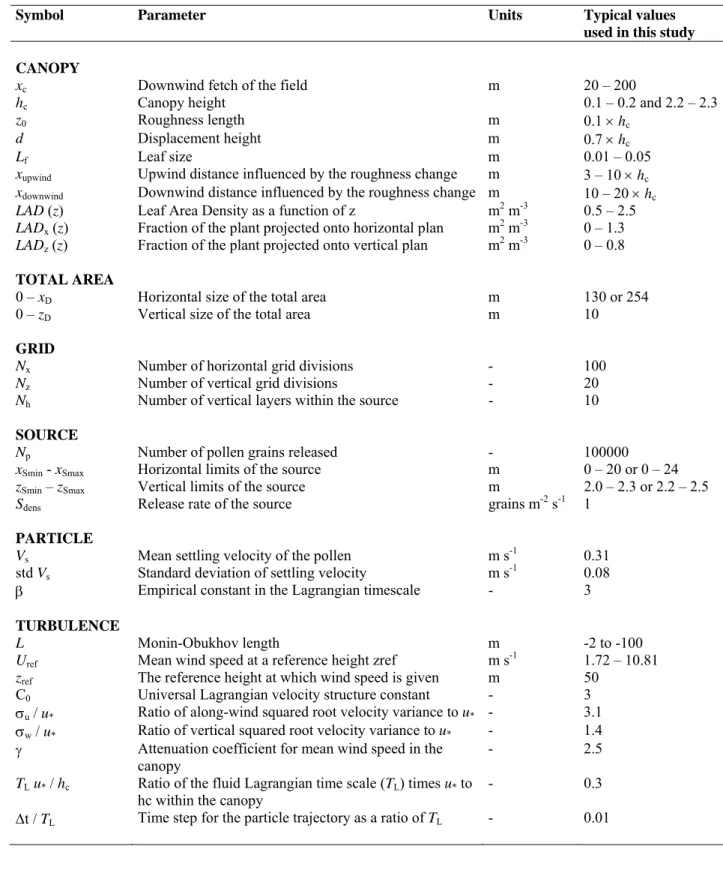
Table 1. Main input parameters of the SMOP-2D model, with units and typical values used in this study.

Symbol Parameter Units Typical values

used in this study CANOPY

xc Downwind fetch of the field m 20 – 200

hc Canopy height 0.1 – 0.2 and 2.2 – 2.3

z0 Roughness length m 0.1 × hc

d Displacement height m 0.7 × hc

Lf Leaf size m 0.01 – 0.05

xupwind Upwind distance influenced by the roughness change m 3 – 10 × hc

xdownwind Downwind distance influenced by the roughness change m 10 – 20 × hc

LAD (z) Leaf Area Density as a function of z m2 m-3 0.5 – 2.5 LADx (z) Fraction of the plant projected onto horizontal plan m2 m-3 0 – 1.3 LADz (z) Fraction of the plant projected onto vertical plan m2 m-3 0 – 0.8

TOTAL AREA

0 – xD Horizontal size of the total area m 130 or 254

0 – zD Vertical size of the total area m 10

GRID

Nx Number of horizontal grid divisions - 100 Nz Number of vertical grid divisions - 20 Nh Number of vertical layers within the source - 10

SOURCE

Np Number of pollen grains released - 100000 xSmin - xSmax Horizontal limits of the source m 0 – 20 or 0 – 24 zSmin – zSmax Vertical limits of the source m 2.0 – 2.3 or 2.2 – 2.5 Sdens Release rate of the source grains m-2 s-1 1

PARTICLE

Vs Mean settling velocity of the pollen m s-1 0.31

std Vs Standard deviation of settling velocity m s-1 0.08

β Empirical constant in the Lagrangian timescale - 3 TURBULENCE

L Monin-Obukhov length m -2 to -100

Uref Mean wind speed at a reference height zref m s-1 1.72 – 10.81 zref The reference height at which wind speed is given m 50

C0 Universal Lagrangian velocity structure constant - 3

σu / u* Ratio of along-wind squared root velocity variance to u* - 3.1

σw / u* Ratio of vertical squared root velocity variance to u* - 1.4

γ Attenuation coefficient for mean wind speed in the canopy

- 2.5

TL u* / hc Ratio of the fluid Lagrangian time scale (TL) times u* to

hc within the canopy - 0.3

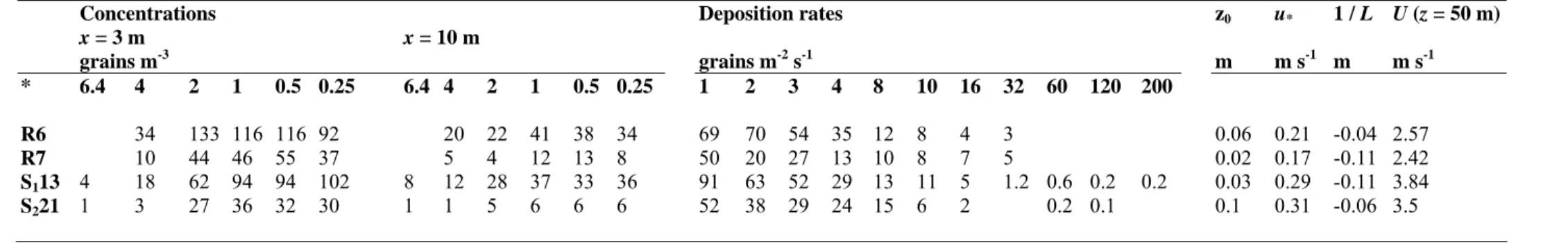
Table 2. Measured concentrations and deposition rates as well as parameters used in the model for each simulation of Figure 3. z0 is the roughness length, u* is the friction

velocity, and L the Monin-Obukhov length over the downwind surface; U(z = 50 m) is the calculated wind speed at z = 50 m over the downwind surface, using the values given in this table for z0, u* and L

Concentrations Deposition rates z0 u* 1 / L U (z = 50 m)

x = 3 m x = 10 m grains m-3 grains m-2 s-1 m m s-1 m m s-1 * 6.4 4 2 1 0.5 0.25 6.4 4 2 1 0.5 0.25 1 2 3 4 8 10 16 32 60 120 200 R6 34 133 116 116 92 20 22 41 38 34 69 70 54 35 12 8 4 3 0.06 0.21 -0.04 2.57 R7 10 44 46 55 37 5 4 12 13 8 50 20 27 13 10 8 7 5 0.02 0.17 -0.11 2.42 S113 4 18 62 94 94 102 8 12 28 37 33 36 91 63 52 29 13 11 5 1.2 0.6 0.2 0.2 0.03 0.29 -0.11 3.84 S221 1 3 27 36 32 30 1 1 5 6 6 6 52 38 29 24 15 6 2 0.2 0.1 0.1 0.31 -0.06 3.5 * height z (m) for concentration and downwind distance x (m) for deposition rates.

Transition zone Upwind homogeneous profile U1(x,z) Downwind homogeneous profile U2 (x,z) xupwind xdownwind

upwind field (1) source field (2) downwind field (3)

xc1 xc2 xc3

U (x,z)

0 0.5 1 1.5 2 2.5 3 0 0.5 1 1.5 2 2.5 LAD (m2 m-3) z (m)

FIGURE 2

z (m ) D (gr ai ns m -2 s -1) R6 R7 0 50 100 150 200 250 0 50 100 150 200 250 -70 35 0 35 70 -70 35 0 35 70 0 1 2 3 0 1 2 3 8 6 4 2 0 z (m ) 8 6 4 2 0 150 100 50 0 D (gr ai ns m -2 s -1) 150 100 50 0 S113 -50 0 50 100 150 200 0 2 4 6 z (m ) 6 4 2 0 0 50 100 150 200 250 z (m ) 8 6 4 2 0 D (gr ai ns m -2 s -1) 150 100 50 0 z (m ) 6 4 2 0 z (m ) 6 4 2 0 S221 0 10 20 30 40 50 -50 0 50 100 150 0 2 4 6 z (m ) 6 4 2 0 D (gr ai ns m -2 s -1) 40 20 0 z (m ) 8 6 4 2 0 C (grains m-3_{) x (m) U (m s}-1₎ (a) (b) (c) FIGURE 3

0

2

4

6

-100%

0%

100%

200%

Mean relative error of C

z

(m)

-150% -50% 50% 150% 250% 1 10 100 1000 x (m)

Mean relative error of

D

0 2 4 6 8 0 50 100 150 C (grains m-3 ) z (m) (a) 0 2 4 6 8 0 20 40 60 C (grains m-3 ) z (m) (b) 0 50 100 -50 0 50 100 150 200 x (m) D (grains m -2 s -1 ) (c) FIGURE 6