Effect of override size on forecast value add

EFFECT OF OVERRIDE SIZE ON FORECAST VALUE ADD by

Jeffrey A. Baker

Bachelor of Science, Chemical Engineering, University of Illinois, 1987 Master of Business Administration, University of Michigan-Flint, 1995

SUBMITTED TO THE PROGRAM IN SUPPLY CHAIN MANAGEMENT IN PARTIAL FULFILLMENT OF THE REQUIREMENTS FOR THE DEGREE OF

MASTER OF ENGINEERING IN SUPPLY CHAIN MANAGEMENT AT THE

MASSACHUSETTS INSTITUTE OF TECHNOLOGY JUNE 2018

(c) 2018 Jeffrey A. Baker. All rights reserved.

The author hereby grants to MIT pennission to reproduce and to distribute publicly paper and electronic copies of this thesis document in whole or in part in any medium now known or

hereafter created.

Signature of Author

Signature redacted

Jetrey A. Baker Department of Supply Chain Management May 11 th, 2018

A /

C tif'

d9

bin

trerd

ce

Certified by. Accepted by MASSACHUSETTS INSTITUTE OF TECHNOLOGY

JUN 1 4 2018

LIBRARIES

Signature redacted

/ I/ Prof. Yossi Sheffi / Director, MIT Center for Transportation and Logistics Elisha Gray II Professor of Engineering Systems Professor, Civil and Environmental Engineering

EFFECT OF OVERRIDE SIZE ON FORECAST VALUE ADD by

Jeffrey A. Baker

Submitted to the Program in Supply Chain Management on May 11, 2018 in partial fulfillment of the

Requirements for the Degree of Master of Engineering in Supply Chain Management

ABSTRACT

Business forecasting frequently combines quantitative time series techniques with qualitative expert opinion overrides to create a final consensus forecast. The objective of these overrides is to reduce forecast error, which enables safety stock reduction, customer service improvement, and manufacturing schedule stability. However, these overrides often fail to improve final forecast accuracy. Process mis-steps include small adjustments, adjustments to accurate statistical forecasts, and adjustments to match financial goals. At best, these overrides waste scare forecasting resources; at worst, they seriously impact business performance.

This report offers a framework for identifying overrides that are likely to improve forecast accuracy. A new class of metrics, Dispersion-Scaled Overrides, was developed as an input to the framework. Other inputs included statistical forecast accuracy and auto-correlation. Classification techniques were used to identify whether an override was likely to create forecast value add. These techniques were found to be approximately 80% accurate in predicting success. This result suggests that using Dispersion-Scaled Overrides alongside common forecast accuracy metrics can reliably predict forecast value add. In turn, this can maximize the value that experts add to the business forecasting process.

Thesis Advisor: Dr. Sergio Caballero Title: Research Scientist

Thesis Advisor: Dr. Nima Kazemi Title: Postdoctoral Associate

Acknowledgements

My deep gratitude goes first to Dr. Sergio Caballero, whose guidance led to break-throughs which made this work possible. I'd also like to express my thanks to Dr. Nima Kazemi for his help and

suggestions to improve upon this work.

To Dr. Chris Caplice, Dr. Eva Ponce, Dr. Alexis Bateman, and the entire SCx staff, thank you for your dedication to SCM MicroMasters program, which provided me the opportunity to attend MIT. You were the catalyst for this journey.

To my friends in the very first SCM blended cohort - we are the pioneers! I've never been part of such a diverse, yet cohesive team. My deepest thanks for your friendship and support on our journey. Apropos of our diversity, I express my thanks by saying Thank You. Gracias. Obrigado. Danke. V L) ffiL -3. k44. t 14.. . Terima kasih. Merci. Cnac"6o.

Asante. EUXaPLUTL>.

To my parents and step-parents, Drs. Bob and Margaret Baker, Dr. James Kirchner, and Kathe Kirchner, thank you for teaching me the value of education, and that the quest for knowledge is a life-long endeavor.

To Kim and Matt, we've always told you to make good choices. Education is one of them. Find your passion, follow it relentlessly, and enjoy the journey - at any age. I love you both.

To the love of my life, Chris. Your love and support throughout the years means the world to me, and without you I'd be nothing. You are my candle in the window. I dedicate this work to you.

Table of Contents Abstract ... 1 Acknowledgem ents... 2 Table of Contents... 3 List of Figures ... 5 List of Tables ... 6 1 Introduction ... 7

1.1 Background -Dem and Forecasting... 7

1.2 Research Problem ... 8

1.3 Current Knowledge Gap... 9

1.4 M ethodology ... 9

1.5 Hypothesis... 10

1.6 Sum m ary ... 11

2 Literature Review ... 12

2.1 Forecasting and Supply Chain M anagem ent... 13

2.2 Do Overrides Im prove Accuracy ... .. ... ... ... . . 14

2.3 Data Analysis and M etrics ... 17

2.4 Literature Gap ... 20

3 M ethodology... 23

3.1 Tim e Series Data and Accuracy M etrics... 26

3.2 Tim e Series Decom position and Residual Analysis ... 28

3.3 Autocorrelation... 31

3.4 Dispersion-Scaled Overrides... 31

3.5 Opportunity Indicators ... 33

3.6 Data Review ... 35

3.7 Data M ining Analytics ... 36

3.8 M ethodology Sum m ary... 38

4 Results and Discussion ... 41

4.1 Research Problem ... 41

4.2 Input Data Results ... 42

4.3 Opportunity Indicators... 47

4.5 Sum m ary of Outcom es ... 60 4.6 Im plications of Findings ... ₆₀ 5 Conclusion ... 63 R eferen ces ... 6 5 Appendix A : Data File Structure ... 69 Appendix B: R Code ... 70

List of Figures

Figure 1: M ethodology Data Flow Overview... 25

Figure 2: Sample output from STL procedure... 29

Figure 3: Sample residuals from STL procedure... 30

Figure 4: Histogram of Residuals ... 30

Figure 5: Autocorrelation of residuals ... 31

Figure 6: Override Percent Histogram ... 42

Figure 7: Median FVA, by Quartile... 45

Figure 8: Override Size/Direction vs. FVA ... 46

Figure 9: Classification Tree... 52

Figure 10: Variable Importance Plot... 55

Figure 11: Standard Deviation Scaled Override vs. Forecast Value Add (%)... 59

List of Tables

Table 1: Example of Scaled Override vs. Percent Override ... 21

Table 2: Overview of Data Elements... 35

Table 3: Data Mining - Classification Techniques ... 37

T able 4: C onfusion M atrix ... 37

Table 5: Mean and Median of Override Sizes ... 43

Table 6: Accuracy Metrics for Statistical and Consensus Forecasts ... 44

Table 7: Opportunity Indicators... 48

Table 8: Response and Predictor Variables ... 51

Table 9: Confusion Matrix for Classification Tree Method ... 53

Table 10: Confusion Matrix for Random Forest Method ... 55

Table 11: Confusion Matrix for Boosted Tree Method ... 56

Table 12: Variable Statistical Significance... 57

Table 13: Confusion Matrix for Logistic Regression ... 58

Table 14: Summary of Selected Metrics for Classification Techniques... 58

1 Introduction

Chapter 1 introduces the concept of demand forecasting and the challenges which it presents in the business environment. An overview of time series models and forecast accuracy measures is provided and serves as the basis for defining the research problem. The current knowledge gap in the literature is defined. Finally, a classification framework is proposed, and the research methodology designed to test it is described.

1.1 Background -Demand Forecasting

Demand forecasting is a critical element of supply chain management, and directly impacts a firm's ability to effectively and efficiently meet customer demand (Chopra & Meindl, 2010). Improving forecast accuracy is important because it drives optimum inventory levels, increased manufacturing efficiency, and improved attainment of customer service levels (M. A. Moon, Mentzer, & Smith, 2003).

Time series models are commonly used in business today to create future demand forecasts (Malehorn, 2005). These models utilize historical patterns in trend and seasonality to predict future values. The underlying assumption of time series forecasting is that the past patterns in the data will repeat themselves in the future. If there are new events or changes in the environment, integrating managerial adjustments, known as overrides, often reduce forecast error (Donihue,

1993).

However, there are several contrary studies which suggest overrides to the baseline statistical forecast may introduce bias, increase error, or are unnecessary (Lawrence, Goodwin, O'Connor, & Onkal, 2006; Eroglu & Croxton, 2010). Over-forecasting bias creates excessive inventory,

which increases holding costs and the working capital required to support it. Under-forecasting bias, while rare, creates the potential for stockouts. Because forecast error is directly related to the amount of safety stock required, increased forecast error will either lead to increased safety stock requirements, or reduced service levels at the same inventory level. Unnecessary overrides, which add little or no value, tie up scarce resources which could be better used elsewhere. Creating a classification framework to identify and minimize these forecast errors is the goal of this research.

1.2 Research Problem

Improving final forecast accuracy for products or aggregated groups of products is critical because it drives optimum inventory levels, increases manufacturing efficiency, and improves customer service levels. Despite the benefits of reduced forecast error, there is usually no guidance on which statistical forecasts are critical to review, or the magnitude of the override which is statistically different from the baseline forecast and therefore likely to improve accuracy. The business need for increased forecast accuracy, coupled with the lack of guidance on where to focus, has created common situations. First, overrides to the statistical forecast are made for products where it would have been better to accept the statistical forecast as the final forecast. Second, small overrides are entered, creating a final forecast which is indistinguishable from the statistical forecast due to underlying variation. Both situations represent wasted effort. So, the goal of forecast accuracy improvement must be balanced against the time and effort required.

Given the desire to improve forecast accuracy and large number of potential overrides, the research question then becomes this: Can a framework be created which identifies where efforts could improve forecast accuracy, or where they might add no value at all?

1.3 Current Knowledge Gap

While previous research has investigated the impact that overrides have on forecast accuracy, this research seeks to address two gaps in this field of study. First, there has been no research in scaling overrides based on dispersion measures. Dispersion-scaled overrides (DSO's) take into consideration the underlying variability of the baseline demand, creating a signal-to-noise style of metric. Second, there is no research which attempts to classify overrides as value added or non-value added based upon dispersion-scaled overrides and baseline statistical forecast accuracy.

1.4 Methodology

This research aims to develop a qualitative framework for classifying a proposed override as either value added or non-value added based on dispersion-scaled overrides, baseline statistical forecast

accuracy, and autocorrelation.

To accomplish this, time series data from forecasting triples consisting of actual demand, statistical forecast, and final forecast are required. Based on the accuracy of the statistical forecast and the final forecast, an improvement metric can be calculated. This metric, which reflects the success of the judgmental override, is known as Forecast Value Added (FVA). FVA values can be compared to user-defined FVA thresholds (FVAcrit) to classify overrides as either value added or non-value added (NVA). FVA is the response variable of interest.

Predictor variables fall into two categories. The first is dispersion-scaled overrides. The actual product demand time series may be decomposed into trend, seasonal, and residual components. For the residual component, the dispersion measures of standard deviation, trimmed mean absolute deviation, and median absolute deviation are calculated. The judgmental override is divided by

these measures of dispersion, creating a signal-to-noise relationship between the override and the underlying variability in the time series.

The second category of predictor variables are opportunity indicators. One is autocorrelation in the residuals, which indicate if there is information not captured in the statistical forecast. The others are measures of baseline statistical forecast accuracy - Root Mean Square Percentage Error (RMSPE), Mean Absolute Percent Error (MAPE) and Median Absolute Percent Error (MdAPE).

To analyze the relationship between the Forecast Value Add response variable and the predictor variables, data mining classification techniques are used. Methods include classification tree, boosted tree, random forest, and logistic regression.

1.5 Hypothesis

It is hypothesized that the probability of creating a value-added override increases based on two or three key factors. The first factor is the accuracy of the baseline statistical model. If the statistical forecast is performing poorly, there are probably opportunities to improve upon it. Conversely, a well-performing model will be difficult to improve. The second factor is autocorrelation. If present, it represents information not reflected in a time series model. The third factor is the size of the override compared to the underlying variation. Overrides indistinguishable from the random noise of random are unlikely to add value.

Developing a classification framework which relates dispersion-scaled overrides, baseline forecast accuracy, and auto-correlation to forecast value add will enhance the efficiency and effectiveness of the business forecasting process. Efficiency will increase as small overrides are flagged as non-value added, and no time is spent entering them. Effectiveness will increase as entering an override

which is flagged as non-value add will prompt discussion and further rationalization. Furthermore, this framework will be self-correcting. Success in creating FVA overrides will make it more likely that future overrides are flagged as FVA. Conversely, poor judgement in entering overrides will make it more likely that future overrides will be flagged as non-value added (NVA).

1.6 Summary

Chapter 1 reviewed demand forecasting, provided an overview of time series models and forecast accuracy measures, and defined the research problem and current knowledge gap. The classification framework and the research methodology designed was described. Chapter 2 will provide an extensive review of the literature which is pertinent to this thesis.

2 Literature Review

Business forecasting is viewed as the starting point for supply chain management, especially as manufacturing strategies have transitioned from a push to pull. A pure push strategy is

production-centric, and the manufacturer simply pushes product into the supply chain and attempts to sell it. The more common approach, however, is the customer-centric pull model. Customer demand is the primary driver, and the supply chain must synchronize accordingly.

In this enviromnent, business forecasting is essential to understand customer demand. The better the final forecast represents true customer demand, the better the supply chain will be able to respond. This response must be both effective and efficient. Being effective means that the customer demand is satisfied; being efficient means that the response is done in a cost-effective manner which allows the supply chain to be profitable.

To create an accurate forecast of customer demand, businesses commonly combine quantitative techniques with qualitative expert opinion to create the final consensus forecast. A commonly used quantitative technique is time series modeling, which predicts future demand based on past demand. The name time series derives from the fact that in these models, time is the only driver. Therefore, future patterns of trend and seasonality will look past patterns of demand and

seasonality. To the extent that this assumption holds true, forecasts will be accurate, and the supply chain may be managed to have both an efficient and effective response. However, due to competitive pressures and other business environment changes, this assumption often breaks down and the errors in the statistical forecast increase

It is because of these breakdowns that judgmental overrides from business experts are often, although not always, desirable. However, overrides from these experts often fail to improve final forecast accuracy.

The Literature Review explores academic works in the areas of judgmental overrides to the forecast, error metrics, and forecast value added analysis. It concludes with a discussion of a gap in the literature, which this analysis seeks to fill.

2.1 Forecasting and Supply Chain Management

Forecasting plays a crucial role in supply chain management, as it impacts production scheduling, inventory management, and procurement (Chopra & Meindl, 2010).

To enable an efficient and effective response to customer demand, production scheduling and inventory management require accurate demand information. Accurate forecasts allow optimum synchronization between the manufacturing plan and inventory levels. This is the well-known economic order quantity, where the costs of manufacturing are balanced against the costs of holding inventory. When multiple products are run on the same line, sequence optimization can minimize the costs of sequence-dependent change overs. Conversely, poor demand information creates many issues. Errors in the forecast could cause unplanned schedule changes, creating waste and increased manufacturing costs as schedules are needlessly adjusted. Poor forecasting will result in either stock-out or excess inventory, or perhaps both. Either situation represents

additional costs for a company, and is undesirable from a business standpoint (M. Moon & Alle, 2015). Businesses may avoid the risk of stock-out by carrying additional safety stock, but the amount of required for a given service level is directly impacted by the forecast error (Huang, Hsieh, & Farn, 2011).

Procurement, both short term purchases and long-term capital expenditures, need forecasting to accurately predict requirements. Research by Syntetos, Nikolopoulos, & Boylan (2010)

demonstrated that forecast adjustments which drive error reduction have a significant impact on reducing the inventory level of raw materials. This effect is similar to that discussed above for finished goods. Increased inventory performance may then be used to either decrease inventory level at a consistent service level, or to increase service at the same inventory level.

Based upon the impacts discussed above, there is considerable interest in reducing forecast error. Given the limitations of statistical models, it is desirable to improve accuracy through

judgmental overrides.

2.2 Do Overrides Improve Accuracy?

Judgmental overrides are commonly used in business forecasting, particularly when external factors are likely to create an impact (Fildes, Goodwin, Lawrence, & Nikolopoulos, 2009). The typical business process is to create the baseline statistical forecast automatically in a software tool, and then have the forecast be reviewed by business personnel. While the review process is company specific, it often includes the personnel from the demand management, sales,

marketing, and business leadership functions. The purpose for the review is that while a

forecasting model may incorporate many aspects of demand - such as trend and seasonality - it does not incorporate all influences on demand. The are many influences where human input is desirable. These factors could include insights into competitor actions, customer expansion plans, changing consumer tastes, or a myriad of other influences which are difficult to incorporate into a forecasting model. Judgmental overrides are designed to improve final forecast accuracy by integrating expert opinion into the forecasting process.

The initial contribution to the literature was presented in a series of papers by Mathews and Diamantopolous (Mathews & Diamantopoulos, 1986, 1989, 1992), which documented the impact that judgmental overrides had on forecast error. Mathews & Diamantopoulos (1986) documented decreases in forecast error through judgmental overrides of the baseline forecast. More forecasts were improved than made worse, although it was noted that biased increased. In their 1989 work, they concluded that the effectiveness of forecast overrides was a function of the product, not the individual creating the adjustment. The 1992 study noted marginal

improvements in error reduction and recommended a formal system of reviewing overrides.

Subsequent research by Fildes et al., (2009) investigated the impact of override size and direction upon forecast accuracy. Negative adjustments were found to be more likely to improve forecast accuracy. Positive adjustments were less likely to increase accuracy, and in many cases reduced accuracy. This behavior driven by two factors, the first being optimism bias. Forecasters and others who enter overrides typically want to show increases in demand. As a result, upward revisions are seldom challenged, and final forecast accuracy suffers. Negative adjustments, however, are usually undesirable. They are often challenged and revised to most accurately reflect the business situation, resulting in increased accuracy. The second driver is confusion between the forecast and the business plan. Forecasts are based on data and should be unbiased, while the business plan is aspirational and based on the desires of management. An incorrect, yet unfortunately frequent response is to enter an override to make the forecast match the business plan.

The size of the adjustment also played a critical role. The smallest quartile of adjustments did not reduce error, which represented a waste of the adjuster's time. Large, negative adjustments usually decreased error, across all companies. Large, positive adjustments decreased error in

some companies, but in others they increased the error. Their recommendation was to avoid small adjustments, which were likely due to adjusters seeing false patterns in the data, or the adjuster trying to prove their role is needed in the process. Avoiding small adjustments would free up time. Their work also highlight that wrong-sided adjustments are particularly damaging for forecast accuracy.

Several number of papers were published by Franses and Legerstee. (P. H. Franses & Legerstee, 2009) concluded that 90% of forecasts are adjusted, and that there is a slight preference to upward adjustments. Forecaster overrides were also related to their past override, i.e. they develop consistent habits over time. Another point was that when evaluating the forecast, adjusters fail to realize that past results, which predicts future demand, are already incorporated to some extent into the current forecast. This leads to a double counting effect.

Franses & Legerstee (2010) concluded that experts put too much weight on their adjustments, and that forecast accuracy could be improved by reducing the weights that forecaster adjustments had on the final forecast. Overall, the adjusted final forecasts were no better than the statistical baseline model.

Franses & Legerstee's (2011) study improved upon the 50% model + 50% manager adjustment weighting scheme proposed by Blattberg and Hoch (Blattberg, 1990). Franses and Legerstee suggested incorporating past performance of experts to modify the split ratio. Too novice or too experienced tended to make larger adjustments, and both cases need to be considered in override evaluation.

Expert opinion was found to decrease error where past model perfonnance had been poor, but not in other cases (P. H. Franses & Legerstee, 2013).

2.2.1 Situations Where Overrides Add Value, and Where They Don't

A common issue with forecasting systems is that the ability to enter forecast overrides imply the need to override each forecast. Doing so often leads to increased errors. Goodwin, Fildes, Lawrence, & Stephens (2011) studied the impacts of placing limits on overrides. One group was allowed to enter overrides only during promotional periods, while another was prohibited from making small adjustments to the forecast, which would be deemed wasteful. The results showed that neither prohibiting small adjustments, nor limiting override to promotional periods improved forecast accuracy. The impact was to encourage over-forecasting when small adjustments were disallowed.

Trapero, Pedregal, Fildes, & Kourentzes (2013) showed improvement in accuracy when overrides occur during promotions, but that greater accuracy may be obtained through multi-variate analysis which includes promotional activity as an input variable instead of a qualitative adjustment. However, an ensemble approach of multi-variate modelling and expert opinion could further improve upon forecast accuracy.

Trapero, Kourentzes, & Fildes, (2015) further their work in advancements of multi-variate models as a replacement to expert opinion. Their dynamic regression models demonstrate improved accuracy, which frees up experts. However, they note no commercially available software to enable dynamic regression, leaving business forecasters the choice between multi-variate models and/or expert opinion.

2.3 Data Analysis and Metrics

In this section, common forecasting error metrics are described. Error metrics are needed to evaluate the impact of judgmental overrides on either increasing or decreasing the final forecast

accuracy. Forecast Value Added (FVA) analysis, which leverages error metrics, is then discussed as a technique to evaluate a judgmental override. Finally, seasonal-trend

decomposition using Loess is described as the technique to understand residual variability in a time series - this is the error which cannot be explained by trend or seasonality.

2.3.1 Forecast Accuracy Metrics

Forecast error for time period t, et is the difference between the actual value (At) and the forecasted value (Ft).

et = At - Ft (1)

There are many scale-dependent metrics, including Root Mean Square Error (RMSE), Mean Absolute Error (MAE), and Median Absolute Error (MdAE). While they are useful for

comparing errors in the same data set, they are not appropriate for comparison between data sets.

Percentage error pt is calculated by dividing the error (et) by the actual value A1.

Pt- (2)

Scale-independent metrics based on percentage error are commonly used to compare

performance between products and product groups which are dissimilar in size. Mean Absolute Percent Error (MAPE) is often recommended in textbooks (Bowerman, O'Connell, & Koehler, 2004). However, MAPE represents one of many scale-independent metrics which may be used to evaluate forecast performance. Other variants include Median Absolute Percent Error (MdAPE) and Root Mean Square Percentage Error (RMSPE), and are discussed by Hyndman & Koehler, 2006. RMSPE was also utilized by (P. H. Franses & Legerstee, 2010).

I

RMPE=Actual Demand.

)

RMSPE=

n

Actual Demandi - Statistical Forecast|

Actual Demand (4)

MAPE =

n

|Actual

MdAPE = Median Acua5Dmad

1 Actual Demandi

There are several downsides to using percentage measures however. In the cases of either intermittent demand, or highly skewed demand, the value for actual demand At could become zero; in those instances, pt and these measures would be undefined. Values close to zero will also cause these measures to become over-inflated.

2.3.2 Forecast Value Add

The typical forecasting process includes several steps. The most common first step is the creation of a statistical forecast, which is based on historic demand observations. Once the statistical forecast is generated, it is then distributed to various functions, which create overrides, and ultimately the final consensus forecast.

In his book "The Business Forecasting Deal", John Wiley & Sons, Inc. (2010) Michael Gilliland describes the Forecast Value Add (FVA) concept. FVA measures changes in forecast error at various stages of the forecasting process.

Because any type of qualitative adjustment to the forecast requires effort on the part of the adjuster, it is always a business question if that effort has resulted in a positive impact to the forecast. If not, it has wasted both time and money (Gilliland, 2013)

While the FVA methodology appears straightforward, it is deceptively difficult to implement. Often no guidance is given to the functional personnel who are tasked with adjusting the forecast. In fact, it is often framed as a requirement for adjustments to be made in order to "correct" the statistical forecast, which is often viewed as "always wrong" (Singh, Raman, & Wilson, 2015).

2.3.3 Seasonal-Trend Decomposition using Loess (STL)

Seasonal-Trend Decomposition using Loess (STL) is a method for decomposing time series into seasonal, trend, and residual components. This method was developed by Cleveland et. al (1990), and has since been coded into R.

Hyndman and Athanasopoulos (2013) discuss the several advantages that STL has over

traditional decomposition techniques. STL can handle all types of seasonality, and the seasonal component is allowed to change over time in case where many seasonal cycles are observed. It is robust to outliers, but while the impact on trend and seasonality is minimized, the residuals can be impacted.

2.4 Literature Gap

The literature describes the need to adjust statistical forecasts to maximize final forecast accuracy, and the fact that overrides commonly fail to do that. In addition, several papers describe a high-level relationship between the size of an override and forecast value add. However, the scaling simply ratios the override by the underlying statistical forecast. No

consideration is given to the underlying variability in the time series, or the performance of the statistical forecast.

This research advances the body of knowledge in two key areas. First, it develops a dispersion-scaled override (DSO), which serves as a signal-to-noise ratio for the override. This improves upon the previous methods of scaling by the original forecast.

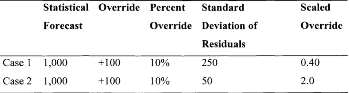
Consider 2 cases listed in Table 1 below. In each case, the statistical forecast is 1,000, the

override is 100, which in both case is a 10% override. However, in case 1, the standard deviation of the residuals is 250. This means that the override of 100 is only 0.4 standard deviation units away. In this case, it's difficult to distinguish the signal from the noise.

In case 2, the standard deviation is 50, which means that the override is 2.0 standard deviations away. This very likely represents a clear signal and should have a higher probability of

increasing the accuracy of the statistical forecast. It is important to note that the initial override must be based on managerial insight or some other expert opinion and must have rational supporting evidence for it.

Table 1: Example of Scaled Override vs. Percent Override

Statistical Override Percent Standard Scaled

Forecast Override Deviation of Override

Residuals

Case 1 1,000 +100 10% 250 0.40

Case 2 1,000 +100 10% 50 2.0

The second advancement is relating the dispersion-scaled override to various predictive

techniques helps support the creation of an override evaluation framework which will be generalizable to business forecasting.

3 Methodology

The methodology chapter describes the approach taken to understand the relationship between forecast value add and several input variables. It first describes using time series data to create the forecast value add response variable. It then describes how time series decomposition is used to create the first class of predictor variables, dispersion-scaled overrides. Standard error and autocorrelation analysis is then used to create the second class of predictor variables. From there, the use of classification techniques to create a framework for relating the response variable to the predictor variable is described. The goal of the framework is to increase the efficiency and effectiveness of the forecasting process.

To address this challenge, a framework was developed to classify proposed overrides as value added or non-values added based on two categories of predictor variables. The data mining techniques of classification tree, boosted tree, random forest, and logistic regression were chosen. These classification techniques have several advantages, including automatic variable selection, robustness to outliers, and no assumptions regarding linearity of relationships between predictor variables and the response variable (Shmueli, Bruce, Yahav, Patel, & Lichtendahl, 2018). In particular, classification trees are attractive because they are graphical in nature and easy to explain to non-technical business personnel.

This framework is appropriate for any company using time series forecasting techniques and managerial overrides. It requires time series forecasting "triples": actual demand, statistical forecast, and final consensus forecast. These triples must be collected at the same level where the override is entered, as that is where the business rationale behind the override is developed and challenged through the consensus process. Typically, the consensus process occurs during sales

and operation planning, but this is not a requirement. If consistency is maintained, any level of the forecasting hierarchy may be used.

The first step in the methodology is to utilize the forecasting triples to create a predictor variable for each set of data points. The actual demand was used to determine the accuracy of statistical and final consensus forecasts. Then, those two accuracy values were compared to create an improvement metric known as Forecast Value Added (FVA). FVA reflects the success of the override in reducing forecast error. FVA was then compared to a user-defined FVA threshold, FVAcrit. Values less than this value are classified as non-value added, while those above the threshold are classified as value added. This is the response variable of interest.

The predictor variables fell into two categories. The first was dispersion-scaled overrides. The actual product demand time series was decomposed into trend, seasonal, and residual components. For the residual component, the dispersion measures of standard deviation, trimmed mean absolute deviation, and median absolute deviation were calculated. The judgmental override was divided by these measures of dispersion, creating a signal-to-noise relationship between the override and the underlying variability in the time series.

The second category of predictor variables were opportunity indicators. One was autocorrelation in the residuals, which would indicate if there was information not captured in the statistical forecast. The others were percentage-based measures of statistical forecast accuracy - Root Mean Square Percentage Error (RMSPE), Mean Absolute Percent Error (MAPE) and Median Absolute Percent Error (MdAPE).

Figure 1 below provides a useful tool to visualize the data flow and connectivity of the various data elements.

Statisdcal

Forecast

Forecast Value override Size CF APE Consensus Forecast D~ecomposition I Dispersion-Scaled Residuals _Overrides

Ro Mean Square RMSE Scaled

Deviation (MAD)d Override

Median Absolute MdAD Scaled Deviation (MdAD) Override

Opportunity Indicators

L) _Statistical

W Forecast Root Mean Square

l'- _{% Error (RMSPE)}

IL

Statistical Mewn Absolute %

< Forecast Error Error (WAE)

U Median Absolute %

i u Actual EDtor (MdAPE

Demand

Figure 1: Methodology Data Flow Overview 0 0 U 0 w LI U) U) L-) 0 5 STL

3.1 Time Series Data and Accuracy Metrics

The starting point of the analysis is the collection of time series data on actual demand, statistical forecasts, and consensus forecast. These can be used to calculate forecast accuracy and forecast value add.

The three time series are collected from the company's system of record, which could be anything from an enterprise resource planning (ERP) system to something as simple as Microsoft Excel. The input data file structure is provided in Appendix A: Data File Structure. Data is typically available within a few business days after month end close. A critical task is to ensure that the data is accurate, as this new data point is used in the generation of the statistical forecast. It was assumed that adequate data management techniques were in place to ensure accuracy of the collected data, as data cleansing is outside of the scope of this effort.

Knowing both the actual demand and the statistical and consensus forecasts, the accuracy of those forecasts may be determined. One commonly used accuracy metric is absolute percent error (APE). Absolute percent error determines the error which exists between a forecast and its actual value. The sign of the error is ignored, as the goal is to reduce the level of error.

|Actualt - Forecastl (6)

Actualt

APE was calculated for both the Statistical and the Consensus forecasts. The difference between them can be used to calculate the Forecast Value Added (FVA) metric. FVA describes how forecast accuracy changes from one step of the forecasting process to the next (Singh, Raman, &

Wilson, 2015). In this analysis, FVA is measured as the change in absolute percent error (APE) that exists between the statistical forecast to the consensus forecast:

FVAt = (APEcons,t - APEstat,t) (7)

FVA was then compared to a user-defined FVA threshold, FVAcit. Values less than this value are classified as non-value added, while those above the threshold are classified as value added. This is the response variable of interest.

Knowing the statistical forecast and the consensus forecast also allows the override size to be calculated. The override is the adjustment to the statistical forecast, and is measured as the difference, in units, between the statistical forecast and the consensus forecast:

Overridet = Consensus Forecastt - Statistical Forecastt (8)

Note that both positive and negative overrides occur and are tracked separately. The override may also be described as a percentage change difference based on the statistical forecast:

Consensus Forecastt - Statistical Forecast (

Statistical Forecaste

The override percent metric is included to allow comparison to earlier work (Fildes, Goodwin, Lawrence, & Nikolopoulos, 2009).

The next step in the methodology is the use of time series decomposition to extract residual error, then calculate dispersion metrics on that error for further use.

3.2 Time Series Decomposition and Residual Analysis

The predictor variables in this research represent signal to noise ratios between an override and the underlying variability of the actual demand time series. It is therefore necessary to decompose the actual demand time series, extract the residuals, and determine their dispersion measures.

Given actual historical demand, a technique called Seasonal-Trend Decomposition using Loess (STL) may be employed to decompose the time series into those trend and seasonal components. An additional set of data, known as residuals, are also computed with this method. The residuals are the errors between the fitted values and the actual historical values of demand.

Dispersion measures were calculated for the residuals, and included root mean square error, trimmed mean absolute deviation, and median absolute deviation. The residuals were also tested for autocorrelation.

3.2.1 Seasonal-Trend Decomposition Using Loess

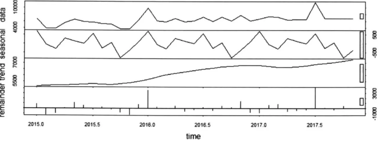
Actual demand (D) was decomposed into the time series components of residual error (e), trend (T), and Seasonality (S) using the Seasonal-Trend decomposition using Loess (STL) procedure (Cleveland, R. B., Cleveland, W. S., McRae, J.E., & Terpenning, I., 1990). STL is part of the "stats v3.4.3" package in R, and is often used to decompose historical demand data (Hyndman, R.J. & Athanasopoulos, G., 2012).

2015.0 2015.5 2016.0 2D16.5 2017.0 2017.5 tMe

Figure 2: Sample output from STL procedure

The output of interest for this research were the residual errors, et. The residual error represents

the difference between the original time series demand data (D) and the seasonal (S) and trend (T) components:

et =-- Dt - Tt - St (10)

Once residuals were obtained, measures of their dispersion were calculated. This provided an

estimate of how much variability there is in the underlying data pattern that cannot be explained

through time series modelling. The values for standard deviation, mean absolute deviation, and median absolute deviation were determined. Their use as scaling factors for overrides is discussed

in section 3.4 below.

Residuals were plotted over time to check that they were homoscedastic, i.e. they will not change over time. See Figure 3 below. Histograms of the residuales were plotted to visually check for a

mean of zero and normal distribution. See Figure 4 below. Note that in many cases there were a

Residuals from STL method C) C0 0) C) C0 0 5 I 10 15 15 20 Period

Figure 3: Sample residuals from STL procedure

Histogram of residuals CD CD--1000 0 1000 2000 outptu$remainder 3000 4000

Figure 4: Histogram of Residuals

Using these residuals, their measures of dispersion were calculated. The measures used were root mean square error, trimmed mean absolute deviation, and median absolute deviation.

0 0 S 0 0 00o 00 0 0 000000 0 0 000 0 0 0 0 0 0 00 0 0 25 30 1 35 Cr 0 L.. I I I .

.

.

.

3.3 Autocorrelation

Another critical check was for autocorrelation, which determines if there is a statistically significant relationship between time-lagged residuals. The presence of autocorrelation suggests there is information which has not been accounted for in the time series model and represents an opportunity for experts to provide a value-added override.

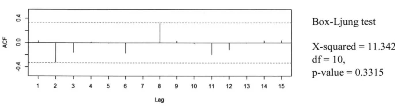
The Ljung-Box test (Ljung & Box, 1978) is implemented in the "stats v3.4.3" package in R, and was used to determine the probability values for autocorrelation. See Figure 5 below. The probability values were used directly in the analysis as predictor variables.

ACF of reskluals C ---- _- -- --- - Box-Ljung test < X-squared = 11.342, df= 10, 9 1 1 Ip-value = 0.3315 1 2 3 4 5 6 7 8 9 10 11 12 13 14 15 Lag

Figure 5: Autocorrelation of residuals

3.4 Dispersion-Scaled Overrides

There are two classes of predictor variables in this research: Dispersion-Scaled Overrides and Opportunity Indicators. In this section, the former will be discussed, while the later will be discussed in section 3.5 below.

The override is the qualitative adjustment, in units, to the statistical forecast, as shown in (9) above. It is performed based on business insights, and the belief that the adjustment represents some

business situation that is not represented by modeling trend and seasonality. Examples include situations such as a new customer, an economic slowdown softening demand, or expansion into a new geography bringing in new demand. To compare the overrides among product groups of varying size, overrides were scaled. The scaling factors were the dispersion measures discussed in section 3.2.1 above; standard deviation, mean absolute deviation, and median absolute deviation. The scaled overrides are analogous to a signal-to-noise ratios and are discussed below.

The first approach is to scale the overrides by dividing through by the standard deviation of the residuals:

Dispersion Scaled Override = (Overridet )1 (r1s)uais

While the standard deviation is a widely used measure of dispersion, it does have the drawback that it is sensitive to outlier values due to the squaring of the error terms.

A second approach is to scale the overrides by dividing through by the Mean Absolute Deviation (MAD) of the residuals. Because the mean is sensitive to outliers, the top five percent of extreme values were trimmed:

Dispersion Scaled Overridet = (Overridet) MADresiduals (12)

A scaled override based on trimmed MAD would be less sensitive to outliers, since the underlying calculation is based on differences rather than the squared differences.

A third approach is to scale the overrides by dividing through by the Median Absolute Deviation (MdAD) of the residuals:

Dispersion Scaled Overridet = (Overridet )/MdADresiduas (13)

A scaled override based on Median Absolute Error would be robust, and less impacted by extreme values.

The final approach to scaling is to simply divide the override by the statistical forecast; this:

Overridet

Forecast Scaled Overridet = Staisi et (14)

Statistical Forecastt

This is a straightforward approach is the technique used in previous studies (Fildes, Goodwin, Lawrence, & Nikolopoulos, 2009). Note that this is not a signal-to-noise ratio style of scaling.

3.5 Opportunity Indicators

Time series models only leverage past actual demand patterns in order to generate a statistical forecast. They assume that future patterns will take a similar form as they have in the past, and that they can be described using only level, trend, and seasonality.

There will also a residual error in every time series statistical forecast. If the error component is large, it is an indication that the time series assumptions have broken down, and that there are other forces at work. As error increases, so does the opportunity for improving upon that error.

For that reason, 3 common measures for the statistical forecast error (Hyndman & Koehler, 2006; Hyndman, R.J. & Athanasopoulos, G., 2012) are included in the analysis. These metrics are calculated for each product group over the entire time horizon and are an indication of how well the statistical model is performing over time. They are also a potential indicator that the model can be improved upon through expert opinion. In other words, a product group with a relatively

high error metrics represents a larger opportunity for improvement versus a more easily forecastable product group with a relatively lower error metrics.

Each of these metrics has been implemented in the functional time series analysis "ftsa vi.1" package in R.

RMSPE =

MAPE =

l Actual Demandi - Statistical Forecasti)2

(Acta Actual Demandi n

Actual Demandi - Statistical Forecastj Actual Demandi

n

(15)

(16)

(17) Actual Demandi - Statistical Forecast

MdAPE = Median Actual Demand

Finally, autocorrelation in the residuals is considered. Autocorrelation exists in time series error data when there is a statistically significant relationship between a value and its own previous historical values. If autocorrelation does exist, it represents an opportunity for improvement that the statistical model cannot capture. The Ljung-Box test for Autocorrelation is coded in R and was used in this analysis.

3.6 Data Review

This section presents an overview of the required data, the accuracy metrics employed, and the two classes of predictor variables used. Table 2 summarizes the data elements.

Table 2: Overview of Data Elements Category

Input Data and Accuracy Metrics Response Variable Time Series Decomposition and Residual Analysis Predictor Variables -Dispersion Scaled Overrides Predictor Variables -Opportunity Indicators Element Actual Demand Statistical Forecast Consensus Forecast Override Size

Absolute Percent Error, statistical and consensus forecasts Forecast Value Add

Residuals

Root Mean Square Error of Residuals (RMSEr) Trimmed Mean Absolute Error of Residuals (trMAE) Median Absolute Error of Residuals (MdAEr)

Scaled Override, Root Mean Square Error

Scaled Override, trimmed Mean Absolute Deviation Scaled Override, Median Absolute Deviation

Forecast Scaled Override

Root Mean Square % Error (RMSPE) of Statistical Forecast Mean Absolute % Error (MAPE) of Statistical forecast Median Absolute % Error (MdAPE) of Statistical forecast Liung-Box test for Autocorrelation

3.7 Data Mining Analytics

Several classification techniques were used to determine the relationship between the forecast value add response variable and the scaled override and opportunity indicator predictor variables. The R programming language was used to perform the analysis; code may be found in Appendix B.

The first step of the analysis was to pre-process the data. The data was randomly partitioned into a training set (60% of data) and testing set (40% of data) then both data sets were scaled based on the training data set. Data partitioning is necessary to avoid over-fitting, and to assess realistically how the model will perform on new data in the future. The 60 training /40 testing partition ratio is found in data mining textbooks (Shmueli et al., 2018).

The second step was to calculate a categorical response variable with only two outcomes. In this study, a threshold value FVAc1 it of 5% was assumed. Any values < = 5% were assigned a 0,

indicating non value added (NVA). Values > 5% were assigned a 1, indicating that there was value added (FVA). In practice, FVAcit would be an input parameter based on a company's definition of value add.

Positive and negative overrides were analyzed separately, as it is hypothesized that larger scaled overrides add value, regardless of sign. Once pre-processing was completed, the data mining techniques shown in

Table 3 below were applied to the training data partition.

Table 3: Data Mining - Classification Techniques

Technique Type Goal

Random Forest

Classification Tree Predict whether an override will create a Boosted Tree Classification Forecast Value Added result greater than the

threshold value of 5% Logistic Regression

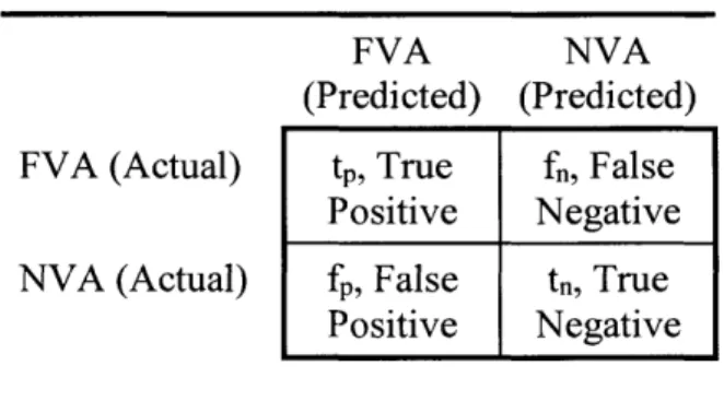
The models created were then evaluated using the data from the testing partition, and a confusion matrix was generated for the predicted versus actual model classifications. See Table 4 below for the generalized confusion matrix format.

Table 4: Confusion Matrix

FVA NVA

(Predicted) (Predicted) FVA (Actual) tp, True f&, False

Positive Negative NVA (Actual) fp, False tn, True

Positive Negative

Given data on correctly classified true positives (tp) and true negatives (tn), and misclassified false positives (fp) and false negatives (fe), various measures of accuracy could be determined.

Accuracy is defined as the overall ability to correctly classify true positives and true negatives, and is calculated as per Equation (18):

tp + tfl

Accuracy = (18)

t, + tn _{+ fp +}

fA

Sensitivity, also known as recall, measure how well the classification method can identify true positives. The calculation is shown in Equation (19):

Sensitivity = tp9)

tP + An

Specificity is the ability to correctly classify false records. The calculation is shown in Equation (20):

Specificity = t (20)

tn + _fp

Precision describes how often the classification is correct when it predicted to be correct. The calculation is shown in Equation (21):

Precision = t (21)

tp + fp

3.8 Methodology Summary

Chapter 3 began by describing the three input time series which serve as the foundation of the analysis -actual demand (D), statistical forecast (SF) and consensus forecast (CF). A fourth time series, override (OVR) was calculated as CF - SF. Comparing the statistical forecast and consensus forecast to the actual demand allowed their absolute percent errors (APESF, APECF) to

be calculated. Calculating the difference between APECF and APESF determined the forecast value add (FVA) of the override. If this value exceeded a threshold value FVAcit, the override was categorized as value added. Otherwise, it was non-value added. This value add / non-value add categorization is the response variable of interest.

To develop a classification framework for the response variable FVA, three categories of predictor variables were created. The first was Dispersion-Scaled Overrides (DSO). The actual demand was decomposed into seasonal (S), trend (T), and residual error (e) components. Dispersion measures of the residual error component - root mean square error (RMSE), mean absolute deviation (MAD), and median absolute deviation (MdAD) - were calculated. Overrides were the divided by these dispersion measures to create DSOs.

The second category of predictor variables was statistical forecast accuracy. The Root Mean Square Percentage Error (RMSPE), Mean Absolute Percentage Error (MAPE) and Median Absolute Percentage Error (MdAPE) of the statistical forecast were calculated.

The final category was autocorrelation of the residuals, which was determined using the Ljung-Box test.

Classification Tree, Boosted Tree, Random Forest, and Logistic Regression were then used to classify overrides as value added or non-value added based on the predictor variables.

Chapter 4 will describe two key areas. The first is an analysis of the input times series, forecast accuracy, and the forecast value add of overrides. The second area is the outcome of the various classification techniques used to relate forecast value add to dispersion-scaled overrides, statistical forecast accuracy, and auto-correlation.

4 Results and Discussion

In this section the results of the analysis are presented. First, information on the input data set is presented, showing the sizes of the adjustments and the accuracy of the statistical and consensus forecasts. Forecast value add, being the response variable of interest, is also presented. The outputs are then discussed. Results from the various data mining approaches are reviewed, beginning with classification techniques before moving on to regression methods.

This chapter concludes by placing the research results from the previous chapter in context with the research problem, and with the broader literature. The results are synthesized, and the implications of those results are discussed. Finally, limitations of this study and recommendations for future work are provided.

4.1 Research Problem

Business forecasting frequently combines quantitative time series techniques with qualitative expert opinion overrides to create a final consensus forecast. The objective of these overrides is to reduce forecast error, which enables safety stock reduction, customer service improvement, and manufacturing schedule stability. However, these adjustments often fail to improve forecast accuracy. Process mis-steps include small adjustments, adjustments to accurate statistical forecasts, and adjustments to match financial goals. At best, these adjustments waste scare forecasting resources; at worst, they seriously impact business performance. The goal of this research was to create a framework for identifying overrides that are likely to improve forecast accuracy.

4.2 Input Data Results

The input to the analysis was monthly time series data at the product group level. Matched sets of forecasting triples - the statistical forecast, the final consensus forecast, and the actual demand

-were collected. The difference, in units, between the monthly values of the statistical and final consensus forecasts allowed the override to be calculated, as per Equation (8) above. The override percent was then calculated by dividing through by the statistical forecast value, as per Equation (9) above. The override percent standardizes the override, allowing comparisons to be made between product lines which differed on an absolute scale. Figure 6 below shows the distribution of overrides from -100% to 200%. The data are right skewed, and 33 of the 703 overrides (4.7%) were greater than 200%.

40-0 C.) 200

-K

4

K

K

Figure 6: Override Percent Histogram 7

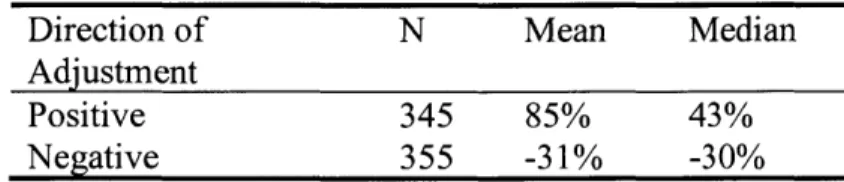
Of the 703 triples collected, only 3 showed no override activity. The 700 overrides were almost equally distributed between positive (n=345) and negative (n=355) adjustments to the statistical forecast (see Table 5 below). Negative overrides were smaller and appear unskewed based on similarities of the median (-30%) and the mean (-31%). However, the positive overrides were larger, and show signs of several very large adjustments which skew the mean (85%) well above the median (43%).

Table 5: Mean and Median of Override Sizes

Direction of N Mean Median

Adjustment

Positive 345 85% 43%

Negative 355 -31% -30%

The skewedness of the positive overrides suggests that an external factor is driving large adjustments and introducing bias into the consensus forecasting process. A likely candidate is the business pressure to have the forecast match the financial objectives of the organization.

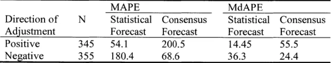
Once the nature of the overrides has been understood, their effect upon the consensus forecast was investigated. To do so, accuracy metrics for both the statistical and the consensus forecasts, as compared to the actual demand, were calculated as per equations (16) and (17) above, and are summarized in Table 6 below. Mean Absolute Percent Error (MAPE) is a commonly used accuracy metric; Median Absolute Percent Error (MdAPE) is less frequently used but is more robust to extreme values.

For positive overrides (n=345), both MAPE and MdAPE increase between the statistical forecast and the final consensus forecast, 54.1% to 200.5%, and 14.5% to 55.5%, respectively. In other words, manual adjustment is causing an increase in the error. This is the opposite of what is

expected and is an indicator that the skewedness observed in the positive override adjustments has had a damaging effect.

For negative overrides (n=355), both MAPE and MdAPE decrease between the statistical forecast and the final consensus forecast, 180.4% to 68.6%, and 36.3% to 24.4%, respectively. This result is as expected; manual intervention by experts should incorporate information unknown to the statistical model, and error should decrease.

Table 6: Accuracy Metrics for Statistical and Consensus Forecasts

MAPE MdAPE

Direction of N Statistical Consensus Statistical Consensus Adjustment Forecast Forecast Forecast Forecast

Positive 345 54.1 200.5 14.45 55.5

Negative 355 180.4 68.6 36.3 24.4

The response variable forecast value add (FVA) was calculated as the pair-wise difference between the absolute present error (APE) of the final consensus forecast minus the statistical forecast, as per equations (6) and (7) above. The FVA median values for positive and negative adjustments were grouped separately, by quartile. The median values based on quartiles is shown in Figure 7: Median FVA, by Quartile, below.

Median FVA Percentage, by Quartile

Override Size Quartile

Figure 7: Median FVA, by Quartile

The smallest 25% _{of both positive and negative overrides (n= 176) had negligible impact on FVA.}

These overrides would fall into the category of time wasters, as the effort put into creating them had no impact on consensus forecast accuracy but did require time.

Negative overrides did show value add, improving the accuracy of the consensus forecast. The second, third, and fourth quartiles showed median accuracy improvements of 18%, 23%, and 78%, respectively. The 78% improvement observed for the largest negative overrides suggest external events which were not predicted by the statistical model but were discerned by the experts entering the override. These results are what would be expected from an expert-opinion based override. The expert has additional information which the statistical forecast does not, and therefore is able to add value. The greater the information gap, the greater the potential for value add. For instance, if a customer goes out of business, sales personnel can immediately remove their demand from the

forecast. In a statistical model, it would take time for that new information to be reflected in the forecast.

Positive overrides resulted in median negative value adds of -23%, -61% and -191% for the second, third, and forth quartiles, respectively. This result is not expected and indicates that something besides additional business information is influencing overrides. The most likely cause of this behavior would be overriding the forecast to equal financial plans. While unexpected, similar results are described in the literature (Baecke, De Baets, & Vanderheyden, 2017; Fildes et al., 2009). Another view of the FVA data is to do so by quadrant, as shown in Figure 8 below. Median values were again used, in order to minimize the impact of extreme values.

Override Size/Direction vs. FVA

Median values per quadrant, with counts

80% 60% -34%, 49%, 217 40% 13%, 6%, 53] 3%,---- , 20% 40% 60 -23%,-13%, 1411 -40%

-60%0

Figure 8: Override Size/Direction vs. FVA

2% _-4-%0

80%

149%, -52%, 2921